Temporal Phase Correction of Multiple Echo T₂ Magnetic Resonance Images

Abstract

Typically, magnetic resonance imaging (MRI) analysis is performed on magnitude data, and multiple echo T₂ data consist of numerous images of the same slice taken with different echo spacing, giving voxel-wise temporal sampling of the noise as the signals decay according to T₂ relaxation. Magnitude T₂ decay data has Rician distributed noise which is characterized by a change in the noise distribution from Gaussian, through a transitional region, to Rayleigh as the signal to noise ratio decreases with increasing echo time. Non-Gaussian noise distributions may produce errors in the commonly applied non-negative least squares (NNLS) algorithm that is used to assess multiple echo decays for compartmentalized water environments through the creation of T₂ distributions. Typically, Gaussian noise is sought by performing spatial-based phase correction on the MRI data; however, these methods cannot capitalize on the temporal information available from multiple echo T₂ acquisitions. Here we describe a temporal phase correction (TPC) algorithm that utilizes the temporal noise information available in multiple echo T₂ acquisitions to put the relevant decay information in the Real portion of the decay data and leave only noise in the Imaginary portion. We apply this TPC algorithm to create real-valued multiple echo T₂ data from human subjects measured at 1.5 T. We show that applying TPC causes changes in the T₂ distribution estimates; notably the possible resolution of separate extracellular and intracellular water environments, and the disappearance of the commonly labeled cerebrospinal fluid peak, which might be an artefact observed in many previously published multiple echo T₂ analyses.

1. Introduction

Various factors in magnetic resonance imaging (MRI), such as magnetic field inhomogeneity, thermal noise, and eddy currents, can cause phase aberrations that introduce noise in the measured real and imaginary k-space values [1]. Consequently, when the k-space data are inverse Fourier transformed into image space, the information will not be entirely real-valued. The typical way of handling the reconstructed MR data in the image domain is to take the magnitude of the complex data and discard the phase information; however, the noise distribution changes from Gaussian to Rician with this operation [1, 2]. These changes in noise distribution are problematic in multiple echo T₂ quantitative image analyses, which generally assume Gaussian distributed noise when analyzed using traditional methods.

Typically, multiple echo T₂ data acquisition consists of measuring the signal intensity of the same anatomical slice with different echo times using a multiple echo spin-echo pulse sequence [3, 4]. The signal intensities of the voxels in the image data will decay exponentially based on the inherent T₂ times, and a T₂ distribution can be created by fitting a sum of exponential decays to the multiple echo decay curve [5]. Multiple echo fitting, using non-negative least squares (NNLS) [5], can be performed to determine the relative proportions of the micro-structural dependent T₂ times [6, 7, 8, 9, 10]. In some cases, such as healthy [3, 4, 11, 12] and pathological [13, 14, 15, 10, 16] central nervous system tissue, different water environments with separate T₂ times are present within a given voxel, resulting in a decay curve from the voxel being the summation of exponential decays from each constituent T₂ time. Four regions are of particular interest: 1) one with a short T₂ time attributed to water trapped between myelin bilayers, called myelin water; 2) one with an intermediate T₂ time attributed to intra- and extracellular water; 3) one with a prolonged T₂ time longer than intra- and extracellular water, which has been noted in pathology [13, 14] and in the corticospinal tract of healthy volunteers [13, 17]; and 4) one with the longest T₂ time in the distribution, or near that of pure water, that is attributed to cerebrospinal fluid.

Ideal multiple echo data consist of high-fidelity decay curves where the final echoes sample only noise. Assuming the noise remains similar for all echoes, this type of data acquisition effectively samples the Rician noise distribution through high to low signal-to-noise ratios (SNRs). Defining noiseless voxel intensities ν and the measured voxel intensities x, the probability distribution of x for Rician distributed noise is [2, 18]

$$p(x\mid \nu ,\sigma )=\frac{x}{{\sigma }^2}exp\left(-\frac{x^2+{\nu }^2}{2{\sigma }^2}\right)I_0\left(\frac{x\nu }{{\sigma }^2}\right)$$ (1)

where I₀ is the modified zeroth order Bessel function of the first kind and σ is the standard deviation of the Gaussian noise, which is assumed to be similar for both real and imaginary components. The SNR can be defined as the ratio of the noiseless voxel intensity divided by the standard deviation of the Gaussian noise, or SNR = ν/σ. Rician noise at different SNR levels are depicted as p_Ri in Fig 1A.

Figure 1.

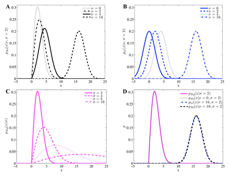
Comparing noise distributions at different SNRs (ν/σ). Rician (A) and Gaussian (B) distributed noise of the same variance, σ², but different mean values, ν. Rayleigh distributed noise with different variances (C). Rician distributed noise compared to Gaussian and Rayleigh distributed noise (D).

When the SNR of the image is sufficiently high, the probability density function of Eqn 1 approaches [2]

$$p(x\mid \nu ,\sigma )\approx \frac{1}{\sigma \sqrt{2\pi }}exp\left(-\frac{{(x-\sqrt{{\nu }^2+{\sigma }^2})}^2}{2{\sigma }^2}\right),$$ (2)

and for high SNR, ν ≫ σ so $\sqrt{{\nu }^2+{\sigma }^2}\approx \nu$, giving

$$p(x\mid \nu \gg \sigma ,\sigma )\approx \frac{1}{\sigma \sqrt{2\pi }}exp\left(-\frac{{(x-\nu )}^2}{2{\sigma }^2}\right),$$ (3)

which is the probability distribution for Gaussian distributed noise with mean ν and standard deviation σ. Gaussian noise distributions for various SNR levels are shown as p_G in Fig 1B. For the cases of high SNR (ν = 16, σ = 2), the Gaussian and Rician distribution curves align quite closely, as shown in Fig 1D.

When the decay reaches the noise-floor, the SNR = 0 and Eqn 1 reduces to [2]

$$p(x\mid \nu =0,\sigma )=\frac{x}{{\sigma }^2}exp\left(-\frac{x^2}{2{\sigma }^2}\right),$$ (4)

which is the probability density function for Rayleigh distributed noise. Various cases of Rayleigh distributed noise are presented as p_Ry in Fig 1C. Equation 4 shows that Rician distributed noise exactly becomes Rayleigh distributed noise for zero SNR. For very low SNR, the Rician distribution approaches the Rayleigh distribution, as shown in Fig 1D.

The presence of noise in the multiple echo T₂ data will influence NNLS fitting [19], but the effect of noise type on T₂ distributions has not been examined. Rician noise can be divided into three segments [2], all of which exist for a magnitude-valued exponential decay that starts with a high SNR and ends with pure noise: 1) high SNR data where the noise is Gaussian distributed; 2) zero SNR data, such as regions of air, where the noise is Rayleigh distributed and can be called the Rayleigh noise floor; and 3) between these two extremes is a transitional region where the noise cannot be described as either Gaussian or Rayleigh distributed. This complicated Rician noise behaviour is not considered when performing multiple echo T₂ decay fitting using NNLS, which assumes the noise to be Gaussian.

It might be tempting to treat the Rayleigh noise floor as a baseline offset in the fitting routine, and introducing a baseline magnetization variable to the NNLS analysis is indeed trivial [5]. However, when a baseline offset is added to the fitting routine, the Rayleigh noise floor is incorrectly treated as such. Misrepresenting the Rayleigh noise floor as a baseline offset is problematic because the baseline value is applied to the entire decay curve. Furthermore, fitting a baseline to the Rayleigh noise floor does not account for the transitional region between Gaussian and Rayleigh noise distributions. A possible solution is to change the noise from Rician to Gaussian, thereby removing the transitional region and the Rayleigh noise floor from the multiple echo decays.

Changing the noise type in MRI data from Rician to Gaussian can be accomplished using phase correction [20, 21]. However, most phase correction methods are designed for data with high SNRs and are performed spatially across the image. The later echoes in some multiple echo T₂ acquisitions reach the Rayleigh noise floor for most tissues, including white and grey matter, but remain above for regions like cerebrospinal fluid, which has a T₂ time close to that of pure water. It is not feasible to apply the same spatially-based phase correction algorithm to each echo-time image, as the phase of a single voxel could change with echo time. Here we developed a phase correction technique that considers the phase temporally, allowing T₂ distributions to be generated from phase-corrected real-valued multiple echo spin-echo data.

2. Methods

2.1. Human Subject Imaging

Multiple echo spin-echo acquisitions were performed on a 1.5-T GE scanner using a transmit-receive, single channel, head coil (GE Healthcare, Milwaukee, WI, USA). A 48 echo single slice acquisition [22] was acquired through the base of the genu and splenium of the corpus callosum in 13 healthy volunteers with the following parameters: 5 mm slice thickness, 128×128 matrix, 22 cm field of view, 10 ms echo spacing for the first 32 echoes and 50 ms for the remaining 16 echoes, 4 averages, transverse acquisition. Composite radio-frequency pulses and crusher gradients were used to eliminate stimulated echoes resulting from spurious signal outside of the selected slice [23]. A variable repetition time was employed: 3.8 s was used for the 20 central lines of k-space and the repetition time was decreased linearly to 2.12 s for the outer lines of k-space. This variable repetition time method reduced scan time substantially with negligible effects on the resulting data [24]. All experimental procedures were approved by local ethics committee at our institution. The multiple echo scans were stored as complex image data. Examples of real-valued and phase images are shown in Fig 2A and 2B. The exponential decay of a white matter voxel is shown in Fig 3, depicting the magnitude, phase, real, and imaginary portions of the original decay.

Figure 2.

Real (A) and phase (B) images of the fourth echo (40 ms) of complex multiple echo MRI data. Minor phase distortions, excluding boundaries and vasculature, can be seen across the images.

Figure 3.

Complex decays shown as magnitude (A), phase (B), real (C), and imaginary (D) valued data from a voxel within white matter. The phase both oscillates and drifts throughout the acquisition.

Regions of interest (ROIs) were drawn bilaterally in the following white matter structures: genu of the corpus callosum, major forceps, minor forceps, splenium of the corpus callosum, and corticospinal tract. The intensity values within the ROI were averaged together for each echo, resulting in a complex, multiple echo decay curve that was then used for analysis. Each white matter ROI was analyzed individually, and data were grouped together for statistical analysis. For each subject, an ROI was drawn in an artefact-free region of air in the magnitude data, which was located by viewing the image at all echoes and adjusting the viewing window/level settings accordingly.

2.2. Temporal Phase Correction

Temporal phase correction of multiple echo MR data was performed using the voxel-wise approach shown in Fig 4 according to the following steps:

Figure 4.

Flowchart of the voxel-wise approach to temporal phase correction of multiple echo MR data.

1. Is voxel intensity > air intensity? If the voxel intensity of the first echo was greater than the mean voxel intensity of the air-ROI, the voxel was assumed to be tissue. This step allowed for determination of voxels inside tissue, thereby reducing computation time.

2. Split into even and odd echoes. The complex voxel decay data was separated into even and odd echoes to account for any even/odd-echo oscillations in the decay data.

3. Unwrap phase. The phase of the complex voxel decay was unwrapped for all echoes greater than the mean voxel intensity of the air-ROI. Once the voxel decay reached the noise-floor, larger jumps in phase are expected and such remaining echoes are excluded from the unwrapping algorithm.

4. Fit 4th order polynomial to the unwrapped phase. A fourth order polynomial was fit to the unwrapped phase of the complex decay to create the zero-phase curve. A fourth order polynomial was chosen empirically, providing a good trade-off between model complexity and computation time. Only voxels with intensity greater than the mean voxel intensity of the air-ROI were used in the polynomial fit, and this process was done for the even and odd echoes separately.

5. Adjust decay using the polynomial as the zero-phase line. The complex data was multiplied by the complex conjugate of the zero phase curve, thereby adjusting the phase of the decay but leaving the magnitude unchanged. Weighting was performed by using a weighted least squares solution that consisted of a vector the same size as the phase data. A vector of ones would cause no weighting. The weighting vector used was 1/n where n is the index of the echo number of the split decay data, causing the early echoes to be weighted more and the later echoes to be weighted less.

6. Recombine even and odd echoes. Recombine the phase corrected, split even and odd echoes into a single decay.

The output of the algorithm was temporally phase corrected complex decay data.

2.3. Analysis

Region of interest drawing and multiexponential analysis was performed on the data using AnalyzeNNLS [25], with the release version 2.5 containing the temporal phase correction scripts in the library and the capability of analyzing either magnitude or real-valued multiple echo T₂ data ¹. The software allows users to adjust the echoes and window/level grey-scale values in the image in order to optimize tissue differentiation.

T₂ distributions were created using 120 T₂ times logarithmically spaced between 0.5 × first echo time and 2 × last echo time, resulting in a range of 5–2240 ms. NNLS was used to fit a basis of T₂ times to the decays [26, 5] and regularization was performed using a generalized cross-validation approach [27, 28].

The relative water fractions and geometric mean T₂ times (gmT₂) were determined for the following T₂ ranges: 1) 5–40 ms for myelin water (MW), 2) 40–100 ms for intra/extracellular water (IEW), and 3) 100–1000 ms for prolonged water (PW), 4) 1000–2240 ms for CSF. These regions were shifted if necessary to assure peak separation.

The corticospinal tract was excluded from the statistical analysis because a PW peak has previously been observed in healthy volunteers [13, 17]. The area fractions determined for the magnitude and TPC data were compared using a one-way ANOVA test for each region where p < 0.0125 was considered statistically significant after Bonferroni correction (p < 0.05/4 = 0.0125).

Representative histograms were made and noise distribution overlays were created for the 8th and 48th echo white matter intensity data from a single subject before and after TPC. The overlays were created by fitting a Gaussian distribution to the temporally phase corrected real-valued data by solving for the mean, ν, and standard deviation, σ, in Eqn 3, and using these values in Eqn 1 to create a Rician noise distributed curve to overlay the original magnitude data. The overlays are for reference only in order to give a qualitative representation of the underlying noise. The 48th echo white matter intensity from all ROIs from all volunteers were grouped together, the mean and standard deviation were determined, and the distribution was compared with a Gaussian distribution with the same mean and standard deviation using a two sample two tailed Student’s T-test.

3. Results

Examples of real-valued and phase images after temporal phase correction are shown in Fig 5 using the same echo shown previously in Fig 2. The real-valued images in Fig 5A no longer exhibit the phase distortions observed in Fig 2A, and the phase images of Fig 5B are uniformly grey, with values near zero, within tissue.

Figure 5.

Real (A) and phase (B) images of the fourth echo (40 ms) of temporally phase corrected complex multiple echo MRI data. The phase within tissue is more uniform than in Fig 2.

The phase maps of all voxels from the fourth echo of Figs 2 and 5 before and after temporal phase correction are shown in Fig 6. Using this phase map representation of grey-scale values in the image, the data are spread out initially (black), and become narrow and centered about the real axis after temporal phase correction (grey). The resulting data does not lie exactly on the line that defines the real axis; this is the expected behaviour from a phase correction algorithm that puts the relevant data in the real channel and leaves only noise in the imaginary channel. An algorithm resulting with data entirely aligned with the real axis is simply the magnitude operation.

Figure 6.

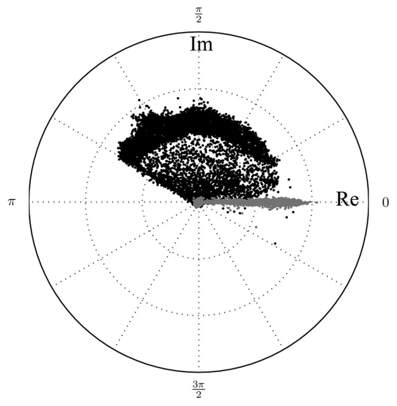
Phase maps before (black dots) and after (grey dots) temporal phase correction for the fourth echo (40 ms) of complex multiple echo MR data.

The decay data from Fig 3 are shown after temporal phase correction in Fig 7. The original phase data are shown as a light grey line in B for reference. After temporal phase correction the phase varies about zero throughout the echoes, and mainly noise appears in the imaginary data (note that the imaginary y axis is on the order of 5, while the magnitude and real data have a y axis of the order of 1000).

Figure 7.

Complex decays shown as magnitude (A), phase (B), real (C), and imaginary (D) valued data from white matter in the same voxel used in Fig. 3 after temporal phase correction. The phase now varies about zero throughout the echoes, and mainly noise appears in the imaginary data. The original phase is shown in light grey in B for comparison.

Representative histograms of grey scale intensities for all of the white matter ROIs from a single volunteer are shown in Fig 8A and B for original magnitude and temporally phase corrected real-valued data for echo 8 and 48, respectively. Gaussian and Rician noise distributions are overlaid for comparison, demonstrating that the underlying noise-profile changed from Rician to Gaussian after temporal phase correction. When all ROIs from all volunteers were averaged together for the 48th echo, the resulting distribution was not statistically different from a Gaussian distribution with the same mean and standard deviation, with p = 0.91.

Figure 8.

Histograms of grey-scale intensities of all white matter ROIs before and after phase correction for a single volunteer (dots) along with fitted distributions (lines). Magnitude values are compared with the phase corrected real values for the 8th echo (A) and 48th echo (B). The noise distributions are barely separated at the 8th echo, while the Rician and Guassian characteristics of the noise are evident for the 48th echo.

Representative T₂ distributions for magnitude and temporally phase corrected decays from each white matter region are shown in Fig 9.

Figure 9.

Representative T₂ distributions in white matter from a single subject from magnitude decays (left column) and a temporally phase corrected decays (right column) for genu (A), major forceps (B), minor forceps (C), splenium (D), and corticospinal tract (E).

The area fractions and gmT₂s of white matter ROIs, excluding the corticospinal tract, using the traditional magnitude data and the temporally phase corrected real-valued data are reported in Table 1. With the exception of myelin water (p = 0.032), significant differences were observed in area fractions between magnitude and temporally phase corrected decays (IEW: p = 1 × 10⁻¹¹, PW: p = 2 × 10⁻¹⁶, CSF: p = 3 × 10⁻⁸³). Out of 104 ROIs, the magnitude data had 8 PW peaks and 104 CSF peaks, while the TPC data had 85 PW peaks and 10 CSF peaks.

Table 1.

Area fractions and geometric mean T₂ times of white matter regions pooled from all subjects, all ROIs using magnitude and temporally phase correction (TPC) analysis approaches. Abbreviations: MW: myelin water; IEW: intra/extracellular water; PW: prolonged water; CSF: cerebrospinal fluid. Standard error shown. ^†8, ^‡85, and *10 of 104 ROIs had these components. The area fractions for MW were note significantly different after temporal phase correction with p = 0.031. The EW, PW and CSF had p ≪ 0.0125. Corticospinal tract ROIs were excluded from this table and statistical comparison.

Fitting Method	Area Fractions
	MW	IEW	PW	CSF
Magnitude	0.096 ± 0.004	0.88 ± 0.01	0.02 ± 0.01†	0.0106 ± 0.0004
TPC	0.080 ± 0.003	0.78 ± 0.01	0.14 ± 0.01‡	0.00008 ± 0.00003*
	Geometric Mean T2 times (ms)
Magnitude	9.3 ± 0.5	76.9 ± 0.9	180 ± 40†	2160 ± 20
TPC	6.9 ± 0.2	69.6 ± 0.7	170 ± 10‡	2120 ± 30*

The area fractions and gmT₂s of corticospinal tract ROIs are presented in Table 2. Out of 26 ROIs, the magnitude data had 20 PW peaks and 26 CSF peaks, while the TPC data had 24 PW peaks and 1 CSF peak.

Table 2.

Corticospinal tract area fractions and geometric mean T₂ times pooled from all subjects, all ROIs using magnitude and temporally phase correction (TPC) analysis approaches. Abbreviations: MW: myelin water; IEW: intra/extracellular water; PW: prolonged water; CSF: cerebrospinal fluid. Standard error shown. ^†20, ^‡24, and *1 of 26 ROIs had these components.

Fitting Method	Area Fractions
	MW	IEW	PW	CSF
Magnitude	0.097 ± 0.009	0.43 ± 0.05	0.46 ± 0.05†	0.019 ± 0.002
TPC	0.096 ± 0.005	0.52 ± 0.03	0.38 ± 0.03‡	0.00004 ± 0.00004*
	Geometric Mean T2 times (ms)
Magnitude	8.9 ± 0.9	56 ± 5	124 ± 3†	2020 ± 60
TPC	8.8 ± 0.6	62 ± 3	168 ± 4‡	2059*

4. Discussion

Phase correction is typically performed spatially [20, 21] where the images contain relatively consistent voxel-wise SNR. However, it is not feasible to apply the same spatially-based phase correction algorithm to each echo-time image, as the phase of a single voxel could change with echo time relative to neighboring voxels. Multiple echo T₂ data contain temporal phase information for each voxel which can be used to correct phase aberrations that introduce noise in the measured complex data. We have successfully implemented a temporal phase correction algorithm that is computationally efficient, easily parallelizable, and effective, as demonstrated by Figs 5–8. A quantitative representation of the spatial phase correction effectiveness by using temporal phase correction is shown in Fig 6. The resulting phase spread has narrowed and lies along the line defining the real axis.

The temporal performance of the TPC algorithm is best demonstrated in the phase (B) and imaginary (D) plots in Fig 7. The resulting phase is centered about zero, with very little variation initially. The values become more erratic for the later echoes, but this is expected because these later echoes correspond to low SNR magnitude signal, where phase noise is expected to increase [2]. The imaginary data after TPC are indistinguishable from noise signal, with the moduli of the TPC imaginary decay data being more than two orders of magnitude smaller than the first echo magnitude intensity in white matter.

Histograms representative of noise distributions for the 8th and 48th echo before and after TPC are shown in Fig 8 for white matter. The fitted distributions give a qualitative representation of the underlying noise. In Fig 8A, the decay signal is much higher than the noise and TPC has very little affect on the histogram. The Gaussian and Rician noise distribution overlays nearly match. Most notably, after TPC, the Gaussian distribution overlay nicely fits the histogram data shown in Fig 8B, and is centered near zero, which is what is expected for real-valued random noise data that has reached the noise floor.

Statistical analysis comparing the TPC histogram to a Gaussian distribution was only performed on the 48th echo, averaging all white matter ROIs together from all volunteers. Noise-floor data were used instead of an earlier echo for the following reasons. Each ROI contains about 30 voxels, which is far too few to get a good comparison with a noise distribution. Averaging all of the ROIs for a single volunteer increases the sampling to 200–400 voxels, but when the signals are not from the noise floor, each region will have a different grey-scale value based on its water content and T₂ decay [6]. So the histogram shown in Fig 8A is made up of several sparsely sampled histograms from different white matter regions, each with different means. Consequently, a good statistical fit to a Guassian distribution is not expected. However, when the signal has reached the noise floor, which is the case for the 48th echo, the mean value should be near or at zero, leaving only noise. And since the same scanner and acquisition was used for all exams, it is reasonable to assume that the standard deviation of zero signal will be the same for all scans. Averaging values from all volunteers gave 5001 voxels, which allows for a strong statistical analysis. Performing a two tailed Student’s T-test gave p = 0.91, indicating the Gaussian distribution curve was not statistically different from the data.

The area fractions of IEW, PW, and CSF peaks were significantly different after temporal phase correction. Representative T₂ distributions are shown in Fig 9. Previous research suggested that changing the noise type from Rician to Gaussian would have dramatic effects on the measured MWF [19]; most notably an increase in MWF would occur as SNR decreases. No significant change was observed for the data presented here in Table 1. However, changes in the MW area fraction could be influenced by the changes in the other three peaks, most notably the appearance of a consistent PW peak in the TPC data, increasing from 8 to 85 occurrences in 104 ROIs (excluding corticospinal tract ROIs), and the essential disappearance of the CSF peak, which was present in all magnitude data and in only 11 of 130 ROIs in the TPC data (including corticospinal tract).

Bjarnason et al also noted changes in the IEW gmT₂ with noise type: Rician noise caused a reduction in IEW gmT₂ when compared to Gaussian noise [19]. The data presented here show that the IEW gmT₂ is longer when comparing Rician distributed noise data with Gaussian distributed noise data. However, it should be noted that Bjarnason et al’s simulations were performed without considering how the presence of a PW peak would affect IEW gmT₂.

For human brain T₂ distributions, peaks with a T₂ time greater than 1 s have long been attributed to CSF [6]. In the data presented here, the CSF peak is present in all magnitude data analysis, and is only present in 11 of 130 ROIs after TPC. This long peak could be attributed to the Rayleigh noise floor, as the fitting algorithm attempts to fit the Rayleigh noise floor with the longest T₂ time in the basis, resulting with a clustering of CSF peaks at the longest T₂ time in the basis: 2240 ms in these analyses. Removing the Rayleigh noise floor eliminated the CSF peak in TPC data analysis; therefore TPC analysis removes a potential artefact commonly assigned to CSF from decay data that does not contain CSF. Consequently, if the decay data are collected such that the noise floor is not reached, this Rayleigh noise floor artefact should be absent, which could explain the absence of the CSF peak in tumor and normal rat brain at 7 T [10] and a 9.4 T study of murine spinal cord [16].

The consistent appearance of a prolonged peak with a gmT₂ around 170 ms was not expected, although there is precedence. Laule et al observed prolonged peaks in pathological normal appearing white matter of both phenylketonuria and multiple sclerosis patients, which they attributed to possibly arising from vacuoles or lesion extracellular water, respectively [13]. However, these prolonged peaks in pathological white matter had gmT₂ times greater than 200 ms and can be ruled out as the source of prolonged peak in the data presented here.

A prolonged peak in the corticospinal tract was previously observed by Russell-Schulz et al [17] with a T₂ of about 120 ms, and it was because of this previous observation that the corticospinal tract ROIs were excluded from Table 1 and the statistical analysis. The gmT₂ of the prolonged peak of the corticospinal tract was found to be 124 ± 3 ms before, and 168 ± 4 ms after TPC, which was comparable to the other white matter structures having a prolonged water gmT₂ time of 170 ± 10 ms after TPC. The prolonged peaks from the white matter structures are probably from a common tissue environment; some physical aspect of the corticospinal tract such as a relatively large PWF or decreased exchanged between the extracellular and intracellular water compartments or increased extracellular water when compared to other white matter structures [17] allows resolution of the prolonged peak using magnitude analysis.

The most likely explanation for the frequent observation of a prolonged signal in the TPC data is that TPC improves the quality of the decay curve to allow for resolution of this peak. In particular, changing the noise distribution from Rician to Gaussian by removing the Rayleigh noise floor and eliminating the transitional region from the decay data, allows for the extracellular and intracellular water pools to be resolved separately by the inversion algorithm. This assertion is further explored in the Appendix where T₂ distributions were generated using TPC decay data by changing the contribution of Rician noise by varying the imaginary valued signal in 5 cases, which affected the T₂ distribution as shown in Fig 11. As the decay data were converted to magnitude, and different levels of imaginary noise contributions were added, the extracellular and intracellular water peaks moved closer together and merged and the CSF area fraction increased with imaginary noise signal contribution.

Figure 11.

T₂ distributions from the minor forceps of a single volunteer using TPC real, S_A (A); magnitude of TPC real, S_B (B); magnitude of TPC real and 33 % of the imaginary channels, S_C (C); magnitude of TPC real and 66 % of the imaginary channels, S_D (D); and magnitude of TPC real and imaginary channels, S_E (E). A and E in this figure are identical to Fig 9C.

Previously, splitting of the IEW peak was observed by Bjarnason et al in NMR studies of bovine white matter using echo spacings of 200 and 400 μs with the final echoes at 736 and 1728 ms, respectively (see Fig 3 in [29]), although no comment was made of this finding in the article. In a carefully designed NMR experiment of rat optic nerve by Bonilla & Snyder, they also observed a splitting of the IEW peak, and assigned the longer peak to intracellular water based on cell swelling [9]. Splitting of the IEW peak has also been observed in peripheral nervous system tissue [8, 30, 31, 32], and Wachowicz & Snyder assigned the longer component to interaxonal water [8], while Webb et al postulated that the longer peak was due to connective tissue [32].

The previous examples of IEW peak splitting reported in the literature occurred almost exclusively in NMR experiments. The resolution limit that defines the minimum ratio of T₂ times that can be resolved is noise dependent such that the higher the SNR, the better the resolution limit [33]. The SNR after TPC is slightly improved because the real-valued decay data are retained and the imaginary-valued data, which should contain mainly noise, is discarded. However, the increased resolution limit in our study most likely resulted from improving the quality of the decay curve by removing the Rayleigh noise floor and transitional region from the decay curve before solving for the T₂ distribution.

The TPC method outlined in this work was developed using data from a single transmit-receive head coil. To apply this technique to multiple coil systems, one can pre-process the data for each receive coil separately, prior to combining the data into a single set of decay images. Getting access to the raw data will depend on the scanner vendor. Applying TPC to data collected using parallel imaging or compressed sensing techniques will likely pose some challenges; such application is beyond the scope of this article, and could be a direction of future work.

Spatial-based phase correction algorithms, such as the statistical methods developed by Ahn & Cho [20] and enhanced by Chang & Xiang [21], are ideal for high SNR MR images. However, applying spatial-based techniques on multiple echo T₂ data, which is essentially made up of the same image at multiple T₂ weightings, suffers limitations under the following two implementations: sequential and projected. The sequential method involves applying the algorithm across the image for each echo. However, later echoes have low SNR in white and grey matter, but high SNR in CSF. Consequently, spatial-based phase correction methods will be dominated by signal from CSF, which is generally of no interest in studies focusing on white and grey matter. Furthermore, if signal from white and grey matter reach the Rayleigh noise floor in the later echoes, spatial-based phase correction methods will cause no change in the tissues of interest, being unable to differentiate tissue from regions of air. Projected methods of phase correction use a spatial-based method on the first and second echo, and then propagate the phase correction on a voxel-wise basis for even and odd echoes separately [34]. This method assumes that the phase remains constant through the echoes, which is contrary to the phase drifts observed in the phase graphs in Figs 3B. These sequential and projected methods of spatial phase correction suffer from the same major limitation; they fail to use additional temporal information available from collecting the same slice repeatedly.

5. Conclusion

Temporal phase correction has been successfully applied to multiple echo spin-echo data, allowing T₂ distributions to be created from real-valued decays. The temporal phase correction technique capitalizes on the special property of multiple echo data where the same image is collected at different points in time as the voxel signal decays through T₂ relaxation. By removing the Rayleigh noise floor and transitional region from the multiple exponential decays, the quality of the decays was improved such that a prolonged peak was consistently identified in the temporally phase corrected data; this peak was likely the result of resolving the extracellular and intracellular water pools based on their T₂ times. The improved quality decays also lead to the disappearance of the peak often identified as cerebrospinal spinal fluid, but was likely an artefact of fitting a long T₂ time to the Rayleigh noise floor.

7. Appendix

To explore the effect of Rician noise on the T₂ distribution, a TPC decay from the minor forceps was used. Each voxel, v is made up of an array of decay signals s_v = s_r + js_i, where s_r is the real-valued decay, s_i is the imaginary valued decay, and $j=\sqrt{-1}$. S is the ROI averaged decay and N is the number of voxels in the ROI. Five cases were explored, averaging over all voxels:

1. $S_A=\frac{{\sum }_v{s}_r}{N}$

2. $S_B=\frac{{\sum }_v\sqrt{s_r^2}}{N}$

3. $S_C=\frac{{\sum }_v\sqrt{s_r^2+{(0.33s_i)}^2}}{N}$

4. $S_D=\frac{{\sum }_v\sqrt{s_r^2+{(0.66s_i)}^2}}{N}$

5. $S_E=\frac{{\sum }_v\sqrt{s_r^2+s_i^2}}{N}$

S_A represents TPC data, and S_E is typical magnitude data. The difference of S_A subtracted from S_B through S_E are shown in Fig 10, highlighting that the more signal used from the imaginary portion of the decay, the more positive bias there was on the decay for the later echoes.

Figure 10.

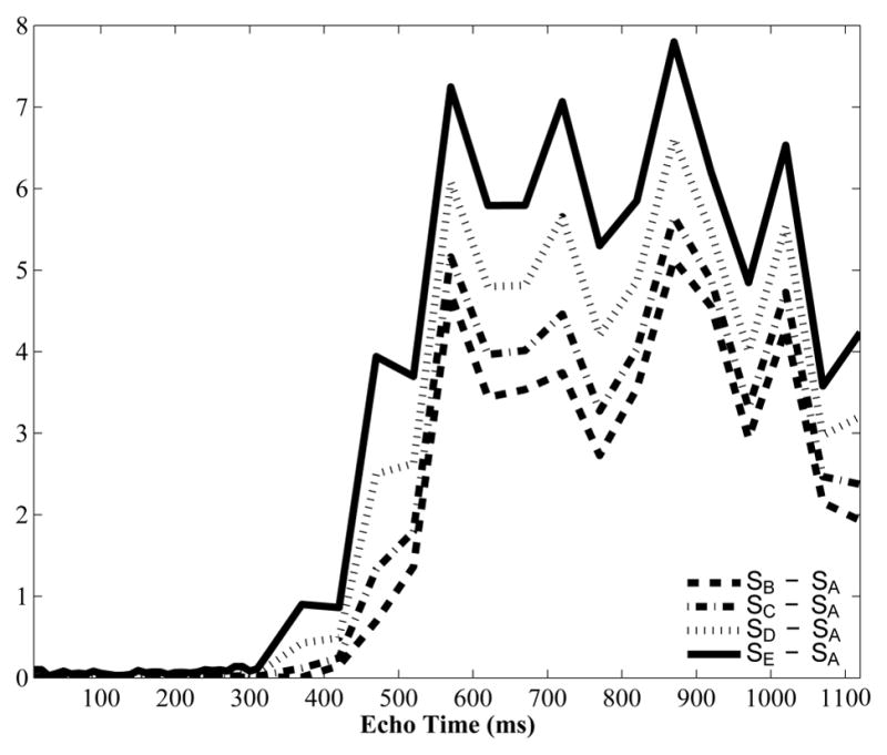
Differences between the TPC real-valued decay data, and magnitude decay data using different levels of contribution from the imaginary channel. The first echo of the decay had a numerical value on the order of 1000.

The resulting T₂ distributions from decay signals S_A to S_E are shown in Fig 11. The T₂ distribution in Fig 11A was from S_A and is identical to the right side of Fig 9C. The CSF area faction was zero. The voxel-wise magnitude operation creating S_B gave the T₂ distribution in Fig 11B. The two central peaks are closer together and the CSF peak has an area fraction of 0.0043. Figure 11C was created from S_C, where 33 % of the imaginary signal contributed to the decay. In this case the middle peaks moved even closer together and the CSF peak area fraction is 0.0049. Increasing the imaginary channel contribution to 66 % caused the middle peaks to partially combine, as shown in Fig 11D, and the CSF contribution increased to 0.0062. Finally, the magnitude of the TPC decay is shown in Fig 11E and is identical to the traditional magnitude approach shown in the left side of Fig 9C. The central peaks are completely combined and the CSF area fraction is the largest at 0.0075. Clearly, increasing the effect of Rician noise in the decays caused the peaks near 100 ms to combine and the CSF peak to appear.

References

- 1.Henkelman RM. Measurement of signal intensities in the presence of noise in MR images. Med Phys. 1985;12(2):232–3. doi: 10.1118/1.595711. [DOI] [PubMed] [Google Scholar]
- 2.Gudbjartsson H, Patz S. The Rician distribution of noisy MRI data. Magn Reson Med. 1995;34(6):910–4. doi: 10.1002/mrm.1910340618. [DOI] [PMC free article] [PubMed] [Google Scholar]
- 3.MacKay A, Whittall K, Adler J, Li D, Paty D, Graeb D. In vivo visualization of myelin water in brain by magnetic resonance. Magn Reson Med. 1994;31(6):673–7. doi: 10.1002/mrm.1910310614. [DOI] [PubMed] [Google Scholar]
- 4.MacKay A, Laule C, Vavasour I, Bjarnason T, Kolind S, Mädler B. Insights into brain microstructure from the T2 distribution. Magn Reson Imaging. 2006;24(4):515–25. doi: 10.1016/j.mri.2005.12.037. [DOI] [PubMed] [Google Scholar]
- 5.Whittall KP, MacKay AL. Quantitative interpretation of NMR relaxation data. J Magn Reson. 1989;84(1):134–52. doi: 10.1016/0022-2364(89)90011-5. [DOI] [Google Scholar]
- 6.Whittall KP, MacKay AL, Graeb DA, Nugent RA, Li DK, Paty DW. In vivo measurement of T2 distributions and water contents in normal human brain. Magn Reson Med. 1997;37(1):34–43. doi: 10.1002/mrm.1910370107. [DOI] [PubMed] [Google Scholar]
- 7.Odrobina EE, Lam TYJ, Pun T, Midha R, Stanisz GJ. MR properties of excised neural tissue following experimentally induced demyelination. NMR Biomed. 2005;18(5):277–84. doi: 10.1002/nbm.951. [DOI] [PubMed] [Google Scholar]
- 8.Wachowicz K, Snyder R. Assignment of the T2 components of amphibian peripheral nerve to their microanatomical compartments. Magn Reson Med. 2002;47(2):239–45. doi: 10.1002/mrm.10053. [DOI] [PubMed] [Google Scholar]
- 9.Bonilla I, Snyder RE. Transverse relaxation in rat optic nerve. NMR Biomed. 2007;20(2):113–20. doi: 10.1002/nbm.1090. [DOI] [PubMed] [Google Scholar]
- 10.Dortch RD, Yankeelov TE, Yue Z, Quarles CC, Gore JC, Does MD. Evidence of multiexponential T2 in rat glioblastoma. NMR Biomed. 2009;22(6):609–618. doi: 10.1002/nbm.1374. [DOI] [PMC free article] [PubMed] [Google Scholar]
- 11.Wu Y, Alexander AL, Fleming JO, Duncan ID, Field AS. Myelin water fraction in human cervical spinal cord in vivo. J Comput Assist Tomogr. 2006;30(2):304–306. doi: 10.1097/00004728-200603000-00026. [DOI] [PubMed] [Google Scholar]
- 12.Minty EP, Bjarnason TA, Laule C, MacKay AL. Myelin water measurement in the spinal cord. Magn Reson Med. 2009;61(4):883–892. doi: 10.1002/mrm.21936. [DOI] [PubMed] [Google Scholar]
- 13.Laule C, Vavasour IM, Mädler B, Kolind SH, Sirrs SM, Brief EE, Traboulsee AL, Moore GRW, Li DKB, MacKay AL. MR evidence of long T2 water in pathological white matter. J Magn Reson Imaging. 2007;26(4):1117–21. doi: 10.1002/jmri.21132. [DOI] [PubMed] [Google Scholar]
- 14.Laule C, Vavasour IM, Kolind SH, Traboulsee AL, Moore GRW, Li DKB, MacKay AL. Long T2 water in multiple sclerosis: What else can we learn from multi-echo T2 relaxation? J Neurol. 2007;254(11):1579–87. doi: 10.1007/s00415-007-0595-7. [DOI] [PubMed] [Google Scholar]
- 15.Laule C, Kozlowski P, Leung E, Li DKB, MacKay AL, Moore GRW. Myelin water imaging of multiple sclerosis at 7 T: correlations with histopathology. NeuroImage. 2008;40(4):1575–80. doi: 10.1016/j.neuroimage.2007.12.008. [DOI] [PubMed] [Google Scholar]
- 16.McCreary CR, Bjarnason TA, Skihar V, Mitchell JR, Yong VW, Dunn JF. Multiexponential T2 and magnetization transfer MRI of demyelination and remyelination in murine spinal cord. NeuroImage. 2009;45(4):1173–1182. doi: 10.1016/j.neuroimage.2008.12.071. [DOI] [PMC free article] [PubMed] [Google Scholar]
- 17.Russell-Schulz B, Laule C, Li DKB, MacKay AL. What causes the hyperintense T2-weighting and increased short T2 signal in corticospinal tract? Magn Reson Imaging. 2012 doi: 10.1016/j.mri.2012.07.003. in press. [DOI] [PubMed] [Google Scholar]
- 18.Rice SO. Mathematical analysis of random noise. Bell System Tech J. 1945;24:46–156. [Google Scholar]
- 19.Bjarnason TA, McCreary CR, Dunn JF, Mitchell JR. Quantitative T2 analysis: The effects of noise, regularization, and multivoxel approaches. Magn Reson Med. 2010;63(1):212–217. doi: 10.1002/mrm.22173. [DOI] [PubMed] [Google Scholar]
- 20.Ahn CB, Cho ZH. A new phase correction method in NMR imaging based on autocorrelation and histogram analysis. IEEE Trans Med Imaging. 1987;MI-6(1):32–6. doi: 10.1109/TMI.1987.4307795. [DOI] [PubMed] [Google Scholar]
- 21.Chang Z, Xiang QS. Nonlinear phase correction with an extended statistical algorithm. IEEE Trans Med Imaging. 2005;24(6):791–798. doi: 10.1109/TMI.2005.848375. [DOI] [PubMed] [Google Scholar]
- 22.Skinner MG, Kolind SH, MacKay AL. The effect of varying echo spacing within a multiecho acquisition: better characterization of long T2 components. Magn Reson Imaging. 2007;25(6):840–7. doi: 10.1016/j.mri.2006.09.046. [DOI] [PubMed] [Google Scholar]
- 23.Poon CS, Henkelman RM. Practical T2 quantitation for clinical applications. J Magn Reson Imaging. 1992;2(5):541–53. doi: 10.1002/jmri.1880020512. [DOI] [PubMed] [Google Scholar]
- 24.Laule C, Kolind SH, Bjarnason TA, Li DKB, MacKay AL. In vivo multiecho T2 relaxation measurements using variable TR to decrease scan time. Magn Reson Imaging. 2007;25(6):834–9. doi: 10.1016/j.mri.2007.02.016. [DOI] [PubMed] [Google Scholar]
- 25.Bjarnason TA, Mitchell JR. AnalyzeNNLS: Magnetic resonance multi-exponential decay image analysis. J Magn Reson. 2010;206(2):200–204. doi: 10.1016/j.jmr.2010.07.008. [DOI] [PubMed] [Google Scholar]
- 26.Lawson CL, Hanson RJ. Solving least squares problems. Prentice-Hall; Englewood Cliffs, NJ: 1974. [Google Scholar]
- 27.Golub GH, Heath M, Wahba G. Generalized cross-validation as a method for choosing a good ridge parameter. Technometrics. 1979;21(2):215–223. doi: 10.2307/1268518. [DOI] [Google Scholar]
- 28.Dula AN, Gochberg DF, Does MD. Optimal echo spacing for multi-echo imaging measurements of bi-exponential T2 relaxation. J Magn Reson. 2009;196(2):149–156. doi: 10.1016/j.jmr.2008.11.002. [DOI] [PMC free article] [PubMed] [Google Scholar]
- 29.Bjarnason TA, Vavasour IM, Chia CLL, MacKay AL. Characterization of the NMR behavior of white matter in bovine brain. Magn Reson Med. 2005;54(5):1072–81. doi: 10.1002/mrm.20680. [DOI] [PubMed] [Google Scholar]
- 30.Does MD, Snyder RE. T2 relaxation of peripheral nerve measured in vivo. Magnetic resonance imaging. 1995;13(4):575–580. doi: 10.1016/0730-725x(94)00138-s. [DOI] [PubMed] [Google Scholar]
- 31.Beaulieu C, Fenrich FR, Allen PS. Multicomponent water proton transverse relaxation and T2-discriminated water diffusion in myelinated and nonmyelinated nerve. Magn Reson Imaging. 1998;16(10):1201–10. doi: 10.1016/s0730-725x(98)00151-9. [DOI] [PubMed] [Google Scholar]
- 32.Webb S, Munro CA, Midha R, Stanisz GJ. Is multicomponent T2 a good measure of myelin content in peripheral nerve? Magn Reson Med. 2003;49(4):638–45. doi: 10.1002/mrm.10411. [DOI] [PubMed] [Google Scholar]
- 33.Istratov AA, Vyvenko OF. Exponential analysis in physical phenomena. Rev Sci Instr. 1999;70(2):1233–1257. doi: 10.1063/1.1149581. [DOI] [Google Scholar]
- 34.van der Weerd L, Vergeldt FJ, de Jager A, Van As H. Evaluation of algorithms for analysis of NMR relaxation decay curves. Magn Reson Imaging. 2000;18(9):1151–1157. doi: 10.1016/s0730-725x(00)00200-9. [DOI] [PubMed] [Google Scholar]