Using Brain Imaging to Extract the Structure of Complex Events at the Rational Time Band

Abstract

A functional magnetic resonance imaging (fMRI) study was performed in which participants performed a complex series of mental calculations that spanned about 2 min. An Adaptive Control of Thought—Rational (ACT-R) model [Anderson, J. R. How can the human mind occur in the physical universe? New York: Oxford University Press, 2007] was developed that successfully fit the distribution of latencies. This model generated predictions for the fMRI signal in six brain regions that have been associated with modules in the ACT-R theory. The model’s predictions were confirmed for a fusiform region that reflects the visual module, for a prefrontal region that reflects the retrieval module, and for an anterior cingulate region that reflects the goal module. In addition, the only significant deviations to the motor region that reflects the manual module were anticipatory hand movements. In contrast, the predictions were relatively poor for a parietal region that reflects an imaginal module and for a caudate region that reflects the procedural module. Possible explanations of these poor fits are discussed. In addition, exploratory analyses were performed to find regions that might correspond to the predictions of the modules.

INTRODUCTION

Newell (1990), in his classic book on unified theories of cognition, noted that human action could be analyzed at different time scales. He identified the biological band as spanning actions that went from approximately 0.1 to 10 msec, the cognitive band as spanning periods from roughly 100 msec to 10 sec, and the rational band as spanning periods from minutes to hours. Cognitive psychology and neuroimaging have both been principally concerned with events happening at the cognitive band. It was at this level that Newell thought the cognitive architecture was most likely to show through. He pointed to studies of things, such as automatic versus controlled behavior (Shiffrin & Schneider, 1977), as fitting comfortably in this range. Neuroimaging techniques also fit within this range not only because they are concerned with typical cognitive psychology tasks but also because their temporal resolution is best suited for this range. They have difficulty discriminating below 10 msec and temporal variability tends to wipe out any pattern much above 10 sec (event-related potential [ERP] tends to fit more the lower range of the cognitive band and functional magnetic resonance imaging [fMRI] the higher end). The question to be pursued in this article is whether analyses of imaging results can be extended to the rational band and whether they will give any insight into processes at this higher level. Newell thought that evidence of the architecture tended to disappear at the larger time scale but, perhaps, that was because of the methodology available at that time.

Much of the recent research in our laboratory (Qin, Anderson, Silk, Stenger, & Carter, 2004; Sohn et al., 2004; Anderson, Qin, Sohn, Stenger, & Carter, 2003) has been directed to extending fMRI techniques to the upper bounds of the Cognitive band, looking at tasks such as algebra equation solving or geometric inference that can take periods of time on the order of about 10 sec. This is a period of time well suited to the relatively crude temporal resolution of fMRI, which is best at identifying events that are a number of seconds apart. We have developed a methodology that involves constructing cognitive models for the tasks in the Adaptive Control of Thought—Rational (ACT-R) cognitive architecture (Anderson et al., 2004) and then mapping the mental steps in the models onto predictions for brain regions. A task that involves visual stimuli and manual responses, like the one studied here, engages six modules in the ACT-R architecture and these have been mapped onto six brain regions:

1. Visual module. We have found that a region of the fusiform gyrus reflects the task-directed visual processing performed by the ACT-R visual module. This region has been shown to be involved in perceptual recognition (e.g., Grill-Spector, Knouf, & Kanwisher, 2004; McCandliss, Cohen, & Dehaene, 2003).

2. Manual module. This is reflected in the activity of the region along the central sulcus that is devoted to representation of the hand. This includes parts of both the motor and the sensory cortex.

3. Imaginal module. The imaginal module in ACT-R is responsible for performing transformations of problem representations. We have associated it with a posterior region of the parietal cortex. This is consistent with other research that has found this region engaged in verbal encoding (Clark & Wagner, 2003; Davachi, Maril, & Wagner, 2001), mental rotation (Heil, 2002; Zacks, Ollinger, Sheridan, & Tversky, 2002; Carpenter, Just, Keller, Eddy, & Thulborn, 1999; Alivisatos & Petrides, 1997; Richter, Ugurbil, Georgopoulos, & Kim, 1997), and visual–spatial strategies in a variety of contexts (Sohn et al., 2004; Reichle, Carpenter, & Just, 2000; Dehaene, Spelke, Pinel, Stanescu, & Tsivkin, 1999).

4. Retrieval module. We have found a region of the prefrontal cortex around the inferior frontal sulcus to be sensitive to both retrieval and storage operations. Focus on this area is again consistent with a great deal of memory research (Cabeza, Dolcos, Graham, & Nyberg, 2002; Fletcher & Henson, 2001; Wagner, Maril, Bjork, & Schacter, 2001; Buckner, Kelley, & Petersen, 1999).

5. Goal module. The goal module in ACT-R sets states that control various stages of processing and prevents the system from being distracted from the goal of a particular stage. We have associated the goal module that directs the internal course of cognition with a region of the anterior cingulate cortex (ACC). There is consensus that this region plays a major role in control (Botvinick, Braver, Carter, Barch, & Cohen, 2001; D’Esposito et al., 1995; Posner & Dehaene, 1994), although there is hardly consensus on how to characterize this role.

6. Procedural module. The procedural module is associated with action selection (where “action” extends to cognitive as well as physical actions). There is evidence (e.g., Frank, Loughry, & O’Reilly, 2001; Amos, 2000; Ashby & Waldron, 2000; Poldrack, Prabakharan, Seger, & Gabrieli, 1999; Wise, Murray, & Gerfen, 1996) that the basal ganglia plays an action-selection role. The region of the basal ganglia that we have selected is the head of the caudate.

This research will test whether these modules show similar systematic involvement in a much more complex and difficult intellectual task than those we have studied so far.

The Task

The research reported here looks at the execution of a rather complex hierarchy of arithmetic computations taking about 2 min. Although many neuroimaging studies have looked at simple arithmetic computations (for a review, see Dehaene, Moiko, Cohen, & Wilson, 2004), only a few studies have been conducted of complex mental calculations. The existing studies (Delazera et al., 2003; Pesenti et al., 2001; Zago et al., 2001) have indicated involvement of parietal and prefrontal regions in organizing the complex computations, but have done little to reveal the role of these regions in the time course of problem solving. They also have not used tasks as complex as the one in the current research.

We chose an artificial task, which required only knowledge of the rules of arithmetic and which could be specified in a way that all participants would decompose it into the same subtasks. This task involved a procedure for recursively decomposing a two-digit number into smaller pairs of numbers until the number can be expressed as a sum of single-digit numbers. Figure 1 illustrates this procedure applied to the number 67. At each level in the figure, the two-digit number n is decomposed into successively smaller pairs of numbers a + b according to the following rules:

1. Find a. This is calculated as half of the number n (rounding down if necessary) plus the tens digit (e.g., in the case of 67 the number a is 33 + 6 = 39).

2. Calculate b as n − a (in the example, 67 − 39 = 28).

3. Decompose a first and then b (this means storing b as a subgoal to be retrieved later).

4. When the decomposition reaches a single-digit number, key it. All digits in the answer were from 5 to 9 and were associated the five fingers on the right hand that were in a data glove.

Figure 1.

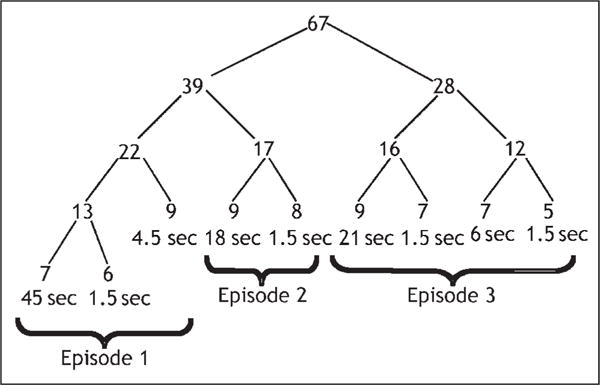
Representation of the decomposition of a number in the experiment. The leaves of the tree give the mean time (rounded to nearest 1.5-sec scan) to generate each number on trials where the participants were correct on the first try. Although the figure illustrates the decomposition of a particular problem, the latencies are averages for all problems.

This is a recursive procedure that decomposes the digits a and b if they are not single-digit numbers. It is a difficult task, as it requires storing and retrieving numbers and performing two-digit arithmetic without paper and pencil. Nonetheless, CMU students could be trained to perform the task with reasonable accuracy. Most of the problems involved generating nine digits, as in this example. Verbal protocols from pilot participants indicated that they were spending much of their time calculating results and also reconstructing past results that they had calculated but lost. As we will see, their latencies are consistent with this general description.

METHODS

Participants

Fourteen normal college students participated in this experiment (right-handed, native English speakers, 19 to 26 years old, average age = 21.5 years, 5 women). They gave written informed consent as approved by the Institutional Review Boards at Carnegie Mellon University and the University of Pittsburgh.

Materials

Ten numbers were chosen in this experiment as starting numbers for the decomposition algorithm. These included the eight possible numbers (59, 61, 62, 63, 64, 65, 66, and 67) that decompose into nine response digits, all five or greater, with the same structure as in Figure 1. To increase variety, we included two numbers (70 and 71) that decompose into 10 digits with a similar structure except that the third digit in Figure 1 is greater than 10 and needs to be decomposed into two digits. For example, the response digits of 70 are 8, 6, 6, 5, 9, 8, 9, 7, 7, and 5. In data analysis, the 3rd and 4th digits were treated as repeated observations of the third digit and the 5th to 10th where treated as 4th to 9th digits. Participants went through as many random permutations of these 10 problems as time allowed.

Procedure

Figure 2 illustrates the structure of a trial. A trial began with a prompt, which was a column of two rectangles with white edges on a black background. The upper rectangle showed a red star, the lower one was empty. After 1.5 sec, the upper rectangle showed the given number and the lower one was empty, waiting for the participant to key in the answer. The digits 5 to 9 where mapped onto the thumb through the little finger on the right hand, which was in a data glove. As the participants keyed in correct digits, the digits accumulated in the bottom rectangle. If a participant hit a wrong key for a digit, a red question mark where the next digit would have appeared and a new try for this digit would start. Participants had up to 300 sec to key in the first digit and 120 sec for each subsequent digit. If they exceeded this time or had 10 failed tries for any digit, the trial would end as an error. When the participant keyed in a new digit correctly, the digit would appear on the screen and the participant would have to wait for the next 1.5-sec scan to begin before they could enter the next digit. All latencies were measured from the beginning of the first scan that they could have entered the digit. After all the digits had been correctly entered, the lower rectangle would disappear, and the upper rectangle would show a white plus sign (+) for 22.5 sec as intertrial interval. On a randomly chosen one-fifth of the trials, the problem terminated after the first response was made. These trials enabled more correct observations on the first digit where more errors were made.

Figure 2.

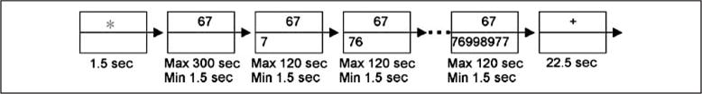
Representation of the structure of an individual trial.

On the day before the scan day, the participants practiced different aspects of the experiment for about 45 min. This session began with key practice with a data glove to familiarize the participants with the keys corresponding to the digits. Then, after studying the instructions for the experiment, the participant practiced decomposing three numbers with seven digits in their answers and one with nine digits in its answer.

fMRI Analysis

Each event-related fMRI recording (Siemens 3 T, echo-planar imaging, 1500 msec TR, 30 msec TE, 55° flip angle, 20 cm FOV with 64 × 64 matrix, 3.125 × 3.125 mm per voxel, 26 slices with 3.2 mm thickness, 0 gap, and with AC–PC in the 20th slice from top) lasted 60 min for three of 20-min blocks with “unlimited” number of trials separated by 15 scans (22.5 sec) of intertrial interval. Each block began with a buffer of four scans (6 sec) during which nothing was presented. These initial scans were discarded in the analysis.

Echo-planar images were realigned to correct head motion using the algorithm AIR (Woods, Grafton, Holmes, Cherry, & Mazziotta, 1998) with a six-parameter rigidbody motion correction. Data were then spatially transformed into a common space using the transformation obtained from coregistering anatomical images to a common reference structural MRI image by means of a 12-parameter automatic algorithm AIR (Woods et al., 1998), and then smoothed with a 6-mm full-width-half-maximum 3-D Gaussian filter to accommodate individual differences in anatomy. Our reference image with Talairach and Tournoux coordinates is available at http://act-r.psy.cmu.edu/mri/. This is the reference brain used for all studies from our laboratory.

All the predefined regions were taken from the translated images after coregistration. As in past research, we used the following definitions of these predefined regions based on prior research (e.g., Anderson, Qin, Yung, & Carter, 2007):

1. Fusiform gyrus (visual): A region 5 voxels wide, 5 voxels long, and 2 voxels high centered at x = ±42, y =−60, z = −8. This includes parts of Brodmann’s area 37.

2. Prefrontal (retrieval): A 5 × 5 × 4 region centered at Talairach coordinates x = ±40, y = 21, z = 21. This includes parts of Brodmann’s areas 45 and 46 around the lateral inferior frontal sulcus.

3. Parietal (problem state or imaginal): A 5 × 5 × 4 region centered at x = −23, y = −64, z = 34. This includes parts of Brodmann’s areas 7, 39, and 40 at the border of the intraparietal sulcus.

4. Motor (manual): A 5 × 5 × 4 region centered at x = ±37, y = −25, z = 47. This includes parts of Brodmann’s areas 2 and 4 at the central sulcus.

5. Anterior cingulate (goal): A 5 × 3 × 4 region centered at x = ±5, y = 10, z = 38. This includes parts of Brodmann’s areas 24 and 32.

6. Caudate (procedural): A 4 × 4 × 4 region centered at x = ±15, y = 9, z = 2.

Except in the case of the motor and prefrontal regions, our experience has been that the effects are nearly symmetric between hemispheres. The response in the motor region is left lateralized because participants are responding with their right hand and the response in the left prefrontal region is much stronger, as is typically found in memory studies for such material. Our analyses will focus on the left regions but we will report their correlations with their right homologues.

RESULTS

Behavioral Data and Model

Table 1 summarizes the behavioral data. It gives the proportion of answers correct on first attempt, the mean time for these correct first attempts, the standard deviation, and the mean number of scans for these correct first attempts. Figure 3 shows separately the distribution of scan lengths for four categories of digits. It takes much longer to key the first digit than any other and Figure 3 shows the flat distribution of number of scans for Digit 1 varying almost uniformly from 0 to 80 scans. Digits 4 and 6 both take about 20 sec and Figure 3 again shows a wide distribution of times but with two thirds of the cases taking 10 scans (15 sec) or less. Digits 3 and 5 both take about 5 sec and Figure 3 shows that a large majority of these observations are under five scans (7.5 sec). Digits 2, 5, 7, and 8 average about a second and Figure 3 confirms that the vast majority of these are brief.

Table 1.

Behavioral Results

Position	Accuracy (%)	Latency (sec)	Standard Deviation (sec)	Scans	No. Correct	Scans	Prediction (sec)
1	80.8	44.87	36.40	30.44	278	30	42.85
2	86.4	0.92	1.85	1.21	246	1	3.81
3	88.9	5.08	13.84	3.45	311	3	9.38
4	83.8	17.78	19.47	12.35	232	12	15.57
5	93.4	1.49	5.58	1.50	253	1	2.21
6	84.8	20.99	19.44	14.48	228	14	19.07
7	91.4	1.18	3.94	1.34	234	1	2.28
8	89.8	5.38	10.27	4.13	228	4	8.30
9	96.8	0.66	0.86	1.08	238	1	1.65

Figure 3.

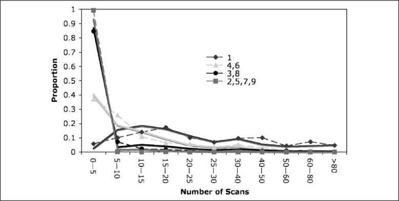
The distribution of number of scans for different digits. Dotted lines connect actual data and solid lines are the predictions of the ACT-R model.

Table 1 and Figure 3 also show the predictions of an ACT-R model.¹ The model averages 99 sec to solve a problem, whereas participants average 97.6 sec. The correlation between that model and the mean latency (Table 1) is .990 and the correlation with the distribution of latencies in Figure 3 is .992.² The ACT-R model for this task was a straightforward implementation of the task instructions. Figure 4 shows the trace of this model (with certain parameter settings that will be explained) performing the task in terms of the activity of the visual module, the retrieval module, the imaginal module, and the manual module. To make this run relatively simple, it was set with parameters that avoid any loss of information or need for recalculation and so it is quite a bit shorter than the average run.

Figure 4.

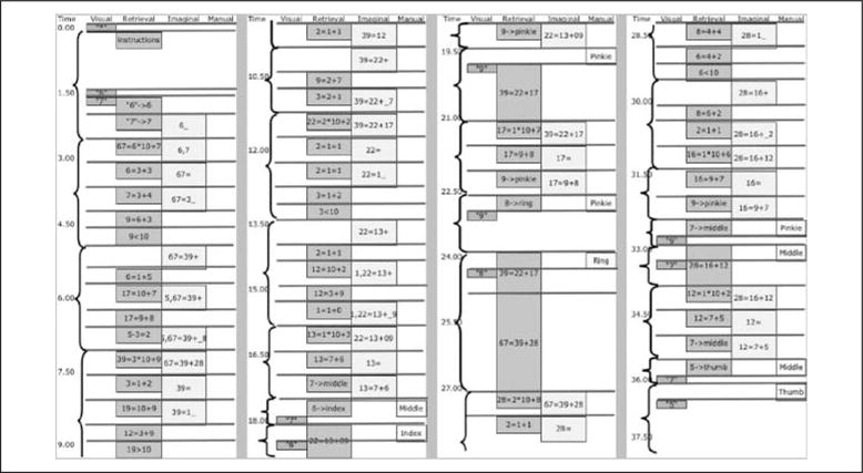
Activation of the visual, retrieval, imaginal, and manual modules in the decomposition of “67.” Time is given in seconds (sec). Lengths of boxes reflect approximate times the modules are engaged. The horizontal lines represent the firing of production rules. Brackets indicate subtasks of activity controlled by a setting of a goal. These subtasks are initial encoding of the problem, calculation of 39 as part of 67, calculation of 28 as the other part, calculation of 22 as part of 39, calculation of 17 as the other part, calculation of 13 as part of 22, calculation of 9 as the other part, special decomposition of 13 into 7 + 6, keying of 7, keying of 6 and retrieval of past decomposition 22 = 13 + 9, keying of 9, retrieval of past decomposition of 39 = 22 + 17, special decomposition of 17 into 9 + 8, keying of 9, keying of 8 and retrieval of past decomposition of 67 = 39 + 28, calculation of 16 as part of 28, calculation of 12 as the other part, special decomposition of 16 into 9 + 7, keying of 9, keying of 7 and retrieval of past decomposition 28 = 16 + 12, special decomposition of 12 into 7 + 5, keying of 7, keying of 5 and processing the end of the trial.

With respect to the module activity:

1. The visual module is activated whenever something appears on the screen including the digits the participants are keying. Although it does not happen in the instance represented in Figure 4, the visual module is also engaged whenever the model needs to recalculate results and so needs to re-encode what is on the screen.

2. The retrieval module is occupied retrieving arithmetic facts, past subgoals, and mappings of digits onto fingers.

3. The imaginal module builds up separate representations of the each digit decomposition. Basically, one image corresponds to each binary branch in Figure 1: 67 = 39 + 28, 39 = 22 + 17, 22 = 13 + 9, 13 = 7 + 6; 17 = 9 + 8; 28 = 16 + 12; 16 = 9 + 7; 12 = 7 + 5.

4. The manual module is activated to program the output of each digit.

5. The procedural module is activated whenever a production rule is selected. These are represented by horizontal lines in Figure 4.

6. The control state in the goal module is reset to control each subtask in the performance of the overall task. The durations of subtasks are indicated by brackets in Figure 4 and the caption to Figure 4 indicates the 23 subtasks illustrated in the figure. In addition, another control state is set for the rest period. These control states are needed to restrict the rules applied to those appropriate for the subtask. Without these control settings, inappropriate rules would intrude and lead to erroneous behavior.

The model run in Figure 4 was designed to avoid all variability in timing for purposes of creating an exemplary run. However, to account for the high variability in times, the following four factors were varied:

1. The durations of the retrievals are controlled by setting a latency parameter in ACT-R randomly according to a uniform distribution on the range 0 to 1.5 sec. The setting in the illustrative run in Figure 4 is 1 sec.

2. The durations of the imaginal operations were also controlled by setting another latency parameter in ACT-R randomly according to a uniform distribution on the range 0 to 1.5 sec. The setting in the illustrative run in Figure 4 is 0.5 sec.

3. The activation threshold was set at −0.5 and the activation noise was set at 0.25. If the activation of a chunk fell below threshold, computation would fail and the system would have to restart. This was particularly likely to happen when past decompositions were being retrieved and particularly in the effort to retrieve 67 = 39 + 28 after the first five digits. In the illustrative run in Figure 4, the retrieval threshold was set so low that no failures of recall could occur in the model.

4. The imaginal representations were lost according to a Poisson distribution such that the losses averaged once every 20 sec. As in factor 3 above, when this happened, the model would have to reconstruct what it was doing.

The errors from (3) and (4) where particularly obvious in participant protocols when they would give up on what they were doing, read the original number (e.g., 67) again, and reconstruct what it was they were suppose to do next.

The predictions displayed in Figure 3 and the predictions that will be displayed for the different module activity are based on averaging 1000 runs for each of the 10 numbers used. The match of the model times to the participant times in Table 1 and Figure 3 is quite good. The goal of the overall modeling enterprise is to use the latency data to estimate the best-fitting parameters and then use these to make predictions about the imaging data. Because we have estimated parameters to fit the latency data, the success at fitting latency is not as strong a test of the model as fitting the imaging data. Nonetheless, in order to give a proper account of the fMRI data, it is important that the model is able to reproduce the distribution of solution times in Figure 3.

Analysis of fMRI Data

Although participants had to repeat their calculations until they got each digit correct, we only analyzed those scans associated with the emission of a correct response on the first attempt. We refer to each sequence of scans ending in a first-attempt correct entry of a digit as a scan sequence. Figure 3 showed the distribution of the lengths of these correct scan sequences. The wide distribution of times poses a challenge for coherently displaying the imaging data and testing the model predictions. As we will describe, the imaging data for each scan sequence were warped to the average number of scans for that position. This then allows the scan sequences to be aggregated. For each participant, we averaged the warped scan sequences to get an average scan sequence for each position for that participant and then averaged these sequences over participants to get the data that are presented.

We tried a number of methods for warping data but in the end found the following gave the most informative results. First, for each trial and each region of interest, we calculated the difference between the blood oxygenation level-dependent (BOLD) response on the scan before presentation of the problem and each subsequent scan in the solution of that problem. We then warped these difference scores for the correct scan sequences to construct a sequence of difference scores for the average length scan sequences for each position. The following is the warping procedure for taking a scan sequence of length n and deriving a scan sequence of the mean length m. It depends on the relative sizes of m and n:

1. If n is greater than or equal to m, create a sequence of length m by taking m/2 scans from the beginning and m/2 from the end. If m is odd, select one more from the beginning. This means just deleting the n − m scans in the middle.

2. If n is less than m, create a beginning sequence of length m/2 by taking the first n/2 scans and padding with the last scan in this first n/2. Construct the end similarly. If either n or m is odd, the extra scan is from the beginning.

This creates scan sequences that preserve the temporal structure of the beginning and end of the sequences and just represent the approximate average activity in their middle.

The nine mean scan sequences involve 67 scans. In addition, a rest period of 15 scans was added at the end to observe how the BOLD response settled to baseline. These scan sequences plus the scan before the problem presentation yield a total of 83 scans for each region of interest. As a final data processing step, we subtracted out any linear drift in across these scans so that the first and last scans were both 0.

Regions of Interest

Figure 5 displays the results for the six predefined regions of interest and the predictions from the six ACT-R modules associated with these regions. The vertical lines in the figure indicate when digits where keyed and identify the boundary of scan sequences. Although we will explain the details of the model fitting and the evaluation in the next section, the match up with the model offers a useful basis for highlighting features of the data. To establish the significance of apparent trends, we included tests for linear and quadratic trends in six portions of the 83 scans. To assess any initial effects, we looked at the first 10 scans, and to assess any effects before the first keypress, we looked at the next 20 scans. There were three bursts of keypresses and we defined three intervals starting with each of these bursts to assess effects associated with these. Finally, we tested the last eight scans to confirm that the BOLD responses had returned to baseline. These tests are reported in Table 2.

Figure 5.

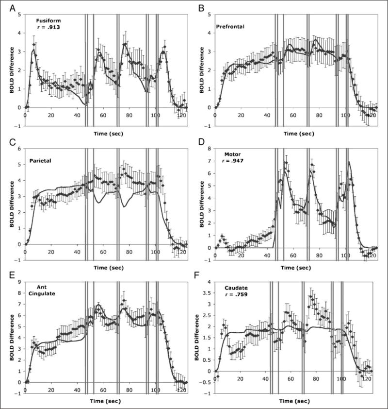
Mean change in BOLD signal for the six predefined regions of the experiment for which ACT-R makes predictions. The mean BOLD responses are displayed along with their standard errors. The solid curve gives the predictions of the ACT-R model. The vertical bars indicate where the nine responses occurred: (A) fusiform (mean BOLD signal 480) reflecting the visual module; (B) prefrontal (mean BOLD signal 463) reflecting the retrieval module; (C) parietal (mean BOLD signal 551) reflecting the imaginal module; (D) motor (mean BOLD signal 476) reflecting the manual module; (E) anterior cingulate (mean BOLD signal 592) reflecting the goal module; and (F) caudate (mean BOLD signal 594) reflecting the procedural module.

Table 2.

Tests for Linear and Quadratic Trends in Various Sequences of the Scan Sequence

Region	Trend	Beginning (Scans 1–10)	Plateau (Scans 11–30)	First Burst (Scans 31–46)	Second Burst (Scans 47–61)	Third Burst (Scans 62–75)	End Scans (76–83)
Fusiform	Linear	2.75		2.28
	Quadratic	5.58		2.95	2.26	2.39
Prefrontal	Linear	6.48	2.27			−4.63
	Quadratic	3.36				2.61
Parietal	Linear	12.40	3.92			−5.20
	Quadratic	9.01				5.13
Motor	Linear		4.72	−3.05	−4.84	−3.33
	Quadratic	2.46		4.43	2.58	6.41
ACC	Linear	5.65	4.81			−4.18
	Quadratic	5.29		2.54		3.47
Caudate	Linear	3.32	4.17
	Quadratic	6.63		2.40	3.22

The t values are only reported if they are at least significant at the .05 level (13 df, two-tailed). A positive value denotes increasing linear trends and convex quadratic trends.

Visual

Figure 5A shows the results for the left fusiform region that corresponds to the visual module in ACT-R. The correlation of the left with the right fusiform is .933. The response in the visual region shows a rise with the presentation of the problem and another rise after each set of numbers is keyed as would be predicted from the visual column in Figure 4. Although the visual column in Figure 4 shows a long period of no activity between reading the target number and keying the first digit, the activity does not go down to zero during this interval. In the model, this is because when it needs to recalculate a result, it has to reread the target number from the screen and such recalculations occur randomly throughout the interval.

Prefrontal

Figure 5B shows the results for the left prefrontal region that corresponds to the retrieval module in ACT-R. The correlation with the left homologous region is .786. As would be predicted from the constant activity in the retrieval column, activity in this region goes up almost immediately and stays at that high level throughout the experiment and starts dropping back to baseline as soon as the last keys are pressed.

Parietal

Figure 5C shows the results for the left parietal region that corresponds to the imaginal module in ACT-R. The correlation with the right parietal is .979. In contrast to the visual and prefrontal regions, the ACT-R model displays some clear misfits to this region. The model predicts dips in parietal activation after the third digit and after the fifth digit. As Figure 4 illustrates, these are places where the model is engaged in response generation and extensive retrieval of prior results and not any imaginal activity. In contrast, if anything, this region shows rises in activation at just these points.

Motor

Figure 5D shows the results for the left motor region where the hand is represented. The correlation with the right motor is .756. It gives a different pattern than the other regions—largely flat until the first responses are given—and shows rises in activation with each burst of responses. The model is quite successful in predicting this region, except for the small activation before the first response where the model predicts no activation. Presumably, this reflects anticipatory hand movements.

Anterior Cingulate Cortex

Figure 5E shows the results for the left ACC, which we think reflects control activity. The correlation with the right ACC is .992. Although it rises to a high level like the parietal and prefrontal, it is distinguished from these regions by showing sharp rises with each response burst. This is predicted by the model in Figure 4 because of the rapid goal changes in the vicinity of these response bursts.

Caudate

Figure 5F shows the results for the left caudate, which we think reflects activity of the procedural module. Its correlation with the right caudate is .986. Although it does rise to a relatively high level like the ACC, it shows extra peaks at the very beginning, after the third response, after the fifth response, and after the ninth response. In contrast, the model, reflecting the rather constant activity of production firing in Figure 4, rises to a steady level and shows little fluctuation. Again, this illustrates evidence that successful model prediction is hardly guaranteed.

Prediction of Regional Activity

Figure 4 provides the information about the activity of six modules. Four of these modules, represented by the columns, each have significant durations of activations according to the ACT-R theory. Two of the modules, the goal module and the procedural module, reflect rather abrupt changes—a production rule takes 50 msec and the ACT-R theory has so far treated control state changes as instantaneous. The formulas for predicting module activity differ depending on whether the modules had point activity, such as the procedural and goal, or whether they had interval activity, such as the visual, retrieval, imaginal, or manual. In either case, we assume that, when active, these modules will create a metabolic demand in their associated regions and produce a hemodynamic response. As is standard in the field (e.g., Friston, 2003; Glover, 1999; Cohen, 1997; Dale & Buckner, 1997; Boyton, Engel, Glover, & Heeger, 1996), we model that hemodynamic response by a gamma function:

$$H(t)=N(a,s)m{(t/s)}^a{e}^{-(t/s)}$$

where m determines the magnitude of the response, a determines the shape of the response, and s determines the time scale. N(a,s) is a normalizing constant and is equal to 1/(s * a!). This function reaches a peak at a * s. We set a = 4 and s = 1.2 sec for all regions. This implies the function reaches a peak at 4.8 sec, which is a typical value. This one hemodynamic function was used for all regions and scaled to the overall level of activity of a region by estimating a separate magnitude parameter. In the case of modules with point activity, we predicted the hemodynamic function at time t by summing the hemodynamic effects of the n points of activity before t:

$$B(t)={\displaystyle \sum _{i=1}^{n}H(t-t_i)}$$

where t_i is the time of the ith activity. In the case of modules with interval activity, the assumption is that the activity is making a constant metabolic demand throughout the interval. If we let D(t) be a 0–1 demand function, indicating whether or not the module is active at time t, then the predicted hemodynamic function can be calculated by convolving this demand function with the hemodynamic function:

$$B(t)={\displaystyle \underset{0}{\overset{t}{\int }}D(x)H(t-x)\mathrm{d}x}$$

The model run represented in Figure 4 is just illustrative and, as discussed with respect to the latency data, the model was parameterized to produce a distribution of times every bit as variable as the participants. The data from the 10,000 simulation problems were broken into scan sequences and these were warped according to the same procedure as used for the data analysis. Note that this means that the warping procedure has the same effects on the predictions as the data—for instance, more accurately representing activity at the beginning and end of sequences. Thus, if we are accurately modeling the processes as they are occurring in the participants, the warped scans should match up between model and data.³

The fits in Figure 5 were obtained by estimating magnitude parameters for each region. These magnitude parameters are provided in Table 3 along with the correlations and a chi-square measure of the goodness of fit. The chi-square is obtained by dividing the difference between each predicted and observed data point by the standard error of the mean for each point (which is indicated in the Figure 4), squaring these values, and summing them. The magnitude parameters were estimated to minimize these chi-square statistics. With 81 points not constrained to be zero and a magnitude parameter estimated, these chi-square statistics have 80 degrees of freedom and any value greater than 102 would be significant at the .05 level. These measures confirm what visual inspection of Figure 4 suggests—the fits to the visual, prefrontal, and ACC regions are quite good and the fits to the parietal, motor, and caudate have problems. It is also the case that all of the visual, prefrontal, and ACC regions are best fit by their associated modules. With two exceptions, trying to fit any other module to these regions results in significant deviations. The exceptions are that the procedural and goal modules yield satisfactory fits to the prefrontal but leave more than twice as much variance unexplained. The deviations for the motor region reflect preparatory motor actions and do not seem particularly interesting, thus we will ignore them. It is also the case that the fit of any other module to the motor region leaves four times or more variance unexplained.

Table 3.

Statistics for Model Fitting

Module:	Visual	Retrieval	Imaginal	Manual	Goal	Procedural
Region:	Fusiform	Prefrontal	Parietal	Motor	ACC	Caudate
Correlation	.913	.977	.832	.947	.956	.759
Magnitude (m)	82.30	8.22	5.06	51.03	9.66	0.98
χ2	38.32	21.17	382.14	186.41	71.40	155.71

Exploratory Analysis

We performed exploratory analyses looking for regions that might display patterns related to the activity of our modules. Analyses that looked for regions whose activity correlated with the overall pattern displayed by a module tended to bring out very large portions of the brain. This is not surprising because all of our modules basically predict increased activation during the task performance and, therefore, will correlate with any region that responds to task structure. We tried multiple regression analyses but the multicollinearity among the predictions of our modules makes it difficult to find regions that reflect a particular module. We did have some success focusing on a particular pattern of variation during the middle of the trial that involves a contrast between modules that predict increased engagement before versus after motor responses. We decided to look at the first burst of three keypresses and the second burst of keypresses, both of which occur during the middle of the task when activation levels tend to be stable. We contrasted the BOLD response over the five scans centered on the last response for each burst (Scans 33–37 and 46–50 in Figure 5)⁴ with the BOLD response over the five scans beginning with the third scan after the response (Scans 38–42 and 51–55 in Figure 5). This creates a maximal contrast between modules that expect a decrease (imaginal, −4%; manual, −18%; goal, −1%) and modules that expect an increase (visual, +12%; retrieval, +11%; procedural, +5%). We performed an exploratory analysis looking for regions of at least 30 contiguous voxels that showed a significant effect of this contrast across participants at p = .01.

Table 4 lists the eight regions identified and the magnitude of the change defined as the difference change in BOLD values from early scans to late scans. It also lists the correlation of each of these regions with the patterns predicted from the visual, manual, and goal modules. The highest correlation between any of these regions and the other modules (retrieval, imaginal, and procedural) was only .655. This analysis found a left motor region, which includes our predefined regions and which correlates with the manual module almost as well as the predefined region. It also uncovered a right motor and a supplementary motor region that correlated strongly with the manual module. The exploratory analysis also found a right prefrontal region that correlated most strongly with the predictions of the goal module (but not nearly as strongly as our predefined ACC regions). It uncovered left and right insula regions that correlated relatively strongly with both the visual and the manual modules. Finally, it uncovered left and right temporal/occipital areas that correlated relatively strongly with the visual module, although not as strongly as the predefined fusiform region. Figure 6 displays the time course of the left motor and left temporal/occipital regions. These two regions correlate least with each other (r = .498) of all the exploratory regions. The motor region does give a profile very much like the predefined region (Figure 5D), but there is a qualitative difference between the patterns displayed by the exploratory temporal/occipital region and the predefined fusiform region (Figure 5A), that is, the exploratory region goes down to baseline after each visual event (initial presentation and appearance of typed digits on the screen), whereas the exploratory region maintains levels above baseline. The model predicts a pattern that corresponds to the predefined fusiform region because, occasionally, it issues top–down requests to encode information when it suffers loss of information due to memory failures or loss of information in the imaginal buffer. The fact that the fusiform reflects this top–down visual activity indicates that it reflects task-relevant visual encoding better than other visual regions.

Table 4.

Areas Found in Exploratory Analyses

Region of Interest	Brodmann’s Area(s)	Voxel Count	Talairach Coordinates			Difference	Correlations
			x	y	z		Visual	Manual	Goal
1. SMA and Cingulate	23/24/32/6	598	0	3	50	−0.47	.814	.883	.589
2. Left motor	1/2/3/4	835	−39	−25	45	−1.37	.746	.932	.828
3. Right motor	1/2/3/4	290	52	−25	33	−0.36	.810	.922	.818
4. Right middle frontal	6/9	42	44	1	39	−0.71	.754	.845	.864
5. R Temporal/Occipital	19, 37	207	44	−59	5	0.40	.869	.666	.437
6. Right insula	13	219	41	9	5	−0.15	.839	.847	.675
7. Left insula	13	391	−30	−6	8	−0.26	.853	.926	.708
8. L Temporal/Occipital	19, 37	88	−39	−64	4	0.40	.864	.589	.429

Figure 6.

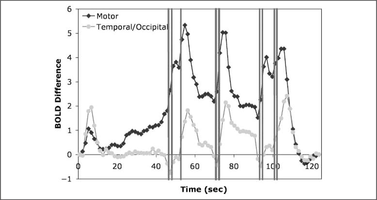
BOLD response in two exploratory regions: left motor (mean BOLD signal 480) and left temporal/occipital (mean BOLD signal 468).

DISCUSSION

This research has shown that it is possible to take a complex task spanning more than a minute, analyze it, and make sense of both behavioral and imaging data. A qualification on this demonstration was that the task involved a set of stimulus onsets and behavioral responses (keying of digits) that partitioned the overall duration into periods that could be given functional significance. The interpretation of the data is anchored around these significant external events. Without these, and in the presence of so much temporal variability, we would have not been able to extract the internal structure of the task. However, many tasks have this structure of breaking up into what Card, Moran, and Newell (1983) called unit tasks. A unit task involves a period of thought ending in a burst of action. Card et al. (1983) identified unit tasks as the major organizational structure at the rational band. Unit task analysis was initially used to characterize text-editing behavior, where each unit task ended in a change to the manuscript. Behavioral research in our laboratory has had a fair degree of success in taking complex tasks, decomposing them into unit tasks, and then applying standard cognitive analyses to the individual unit tasks (e.g., Sohn, Douglass, Chen, & Anderson, 2005; Anderson, 2002; Lee & Anderson, 2001). This article has shown that a unit task analysis also can be applied to imaging data.

With respect to support for the ACT-R theory, the imaging data allowed for strong tests of the model that was developed in that theory and indirectly of the theory itself. After the latency data were used to parameterize the model, the model made predictions for the activity that would be observed in the six predefined regions. The basic shape of the BOLD response for each region was completely determined by the timing of the ACT-R modules and the only parameter estimated in fitting the BOLD response was overall magnitude. The predictions were stronger than what was reflected in the correlation coefficients because the model is also committed to a zero value (this is similar to regression where one only estimates slope and not intercept). By this strong test, the results obtained in the fusiform (visual module), prefrontal (retrieval module), ACC (goal module), and motor regions (manual module) were remarkably good. In addition to confirming the predictions of the ACT-R model, these results are relevant to current issues about the function of the ACC. The activity in the ACC is responding to the overall need for cognitive control in the task and is not just a matter of response conflict (e.g., Botvinick et al., 2001; Carter et al., 2000; MacDonald, Cohen, Stenger, & Carter, 2000) or response to errors (e.g., Falkenstein, Hohnbein, & Hoorman, 1995; Gehring, Goss, Coles, Meyer, & Donchin, 1993). Its general control function seems closer to the proposals of D’Esposito et al. (1995) and Posner and Dehaene (1994).

There were problems with our use of the imaginal module for the parietal and the procedural module for the caudate. The imaginal module is the newest module in ACT-R and is still in development. The module had predicted a decrease in activation with each response burst because the module was not involved in the response generation or the subsequent effort to retrieve a past result. Our exploratory efforts failed to find any brain region with a general profile like the imaginal but which showed decreases at these points. Thus, it does not seem that the problem is with the association of this region with the module. Rather, either the problem is with the model or the underlying theory of the imaginal module. With respect to the model, perhaps we were wrong in assuming that it is not engaged in response generation. Converting digits to fingers may have placed a representational burden. Or perhaps we were wrong in assuming that participants tried to retrieve past results; maybe they immediately tried to reconstruct them. With respect to the theory of imaginal module, we may be wrong in the assumption that it is not engaged in retrieval (for discussions of this issue, see Anderson, Byrne, Fincham, & Gunn, 2008; Wagner, Shannon, Kahn, & Buckner, 2005).

The procedural module failed to predict the pronounced spikes in the caudate that occurred after each burst of keypresses. In contrast to the imaginal module, the procedural module is one of the most established in ACT-R and, as noted earlier, there is general evidence for a procedural involvement of the caudate. However, it is probably unreasonable to expect that caudate activity only reflects this single function. It is known to also reflect reward activities (e.g., Delgado, Locke, Stenger, & Fiez, 2003; Breiter, Aharon, Kahneman, Dale, & Shizgal, 2001) and to respond to eye movements (e.g., Gerardin et al., 2003). The unexpected spikes may reflect these processes. It should be noted that increased caudate fired at episode boundaries has been found in rats (Barnes, Kubota, Hu, Jin, & Graybiel, 2005) and in monkeys (Fujii & Graybiel, 2005). It may be that its activity reflects unit task structure at the level of Newell’s rational band.

Although the results of this research have been mixed with respect to supporting the predictions of the ACT-R model, they seem uniformly positive with respect to the prospect of using fMRI to study the structure of complex tasks. We were able to obtain meaningful data that could confirm predictions of a model (those derived from the visual, retrieval, and goal modules in ACT-R), to suggest ways that a model could be adjusted (adding anticipatory motor programming to the motor module), to suggest places where a theory may need to be changed (results from the caudate and parietal modules), and to identify new regions that may be related to the structure of the task. Provided one can deal with the temporal variability in the performance of such tasks, the temporal resolution of fMRI seems well suited to understanding the structure of tasks that are in Newell’s rational band.

References

- Alivisatos B, Petrides M. Functional activation of the human brain during mental rotation. Neuropsychologia. 1997;35:111–118. doi: 10.1016/s0028-3932(96)00083-8. [DOI] [PubMed] [Google Scholar]
- Amos A. A computational model of information processing in the frontal cortex and basal ganglia. Journal of Cognitive Neuroscience. 2000;12:505–519. doi: 10.1162/089892900562174. [DOI] [PubMed] [Google Scholar]
- Anderson JR. Spanning seven orders of magnitude: A challenge for cognitive modeling. Cognitive Science. 2002;26:85–112. [Google Scholar]
- Anderson JR. How can the human mind occur in the physical universe? New York: Oxford University Press; 2007. [Google Scholar]
- Anderson JR, Bothell D, Byrne MD, Douglass S, Lebiere C, Qin Y. An integrated theory of mind. Psychological Review. 2004;111:1036–1060. doi: 10.1037/0033-295X.111.4.1036. [DOI] [PubMed] [Google Scholar]
- Anderson JR, Byrne D, Fincham JM, Gunn P. The role of prefrontal and parietal cortices in associative learning. Cerebral Cortex. 2008;18:904–914. doi: 10.1093/cercor/bhm123. [DOI] [PMC free article] [PubMed] [Google Scholar]
- Anderson JR, Qin Y, Sohn MH, Stenger VA, Carter CS. An information-processing model of the BOLD response in symbol manipulation tasks. Psychonomic Bulletin & Review. 2003;10:241–261. doi: 10.3758/bf03196490. [DOI] [PubMed] [Google Scholar]
- Anderson JR, Qin Y, Yung KJ, Carter CS. Information-processing modules and their relative modality specificity. Cognitive Psychology. 2007;54:185–217. doi: 10.1016/j.cogpsych.2006.06.003. [DOI] [PubMed] [Google Scholar]
- Ashby FG, Waldron EM. The neuropsychological bases of category learning. Current Directions in Psychological Science. 2000;9:10–14. [Google Scholar]
- Barnes T, Kubota Y, Hu D, Jin DZ, Graybiel AM. Activity of striatal neurons reflects dynamic encoding and recoding of procedural memories. Nature. 2005;437:1158–1161. doi: 10.1038/nature04053. [DOI] [PubMed] [Google Scholar]
- Botvinick MM, Braver TS, Carter CS, Barch DM, Cohen JD. Conflict monitoring and cognitive control. Psychological Review. 2001;108:624–652. doi: 10.1037/0033-295x.108.3.624. [DOI] [PubMed] [Google Scholar]
- Boyton GM, Engel SA, Glover GH, Heeger DJ. Linear systems analysis of functional magnetic resonance imaging in human V1. Journal of Neuroscience. 1996;16:4207–4221. doi: 10.1523/JNEUROSCI.16-13-04207.1996. [DOI] [PMC free article] [PubMed] [Google Scholar]
- Breiter HC, Aharon I, Kahneman D, Dale A, Shizgal P. Functional imaging of neural responses to expectancy and experience of monetary gains and losses. Neuron. 2001;30:619–639. doi: 10.1016/s0896-6273(01)00303-8. [DOI] [PubMed] [Google Scholar]
- Buckner RL, Kelley WM, Petersen SE. Frontal cortex contributes to human memory formation. Nature Neuroscience. 1999;2:311–314. doi: 10.1038/7221. [DOI] [PubMed] [Google Scholar]
- Cabeza R, Dolcos F, Graham R, Nyberg L. Similarities and differences in the neural correlates of episodic memory retrieval and working memory. Neuroimage. 2002;16:317–330. doi: 10.1006/nimg.2002.1063. [DOI] [PubMed] [Google Scholar]
- Card SK, Moran TP, Newell A. The psychology of human–computer interaction. Hillsdale, NJ: Erlbaum; 1983. [Google Scholar]
- Carpenter PA, Just MA, Keller TA, Eddy W, Thulborn K. Graded function activation in the visuospatial system with the amount of task demand. Journal of Cognitive Neuroscience. 1999;11:9–24. doi: 10.1162/089892999563210. [DOI] [PubMed] [Google Scholar]
- Carter CS, MacDonald AM, Botvinick M, Ross LL, Stenger VA, Noll D, et al. Parsing executive processes: Strategic versus evaluative functions of the anterior cingulate cortex. Proceedings of the National Academy of Sciences, USA. 2000;97:1944–1948. doi: 10.1073/pnas.97.4.1944. [DOI] [PMC free article] [PubMed] [Google Scholar]
- Clark D, Wagner AD. Assembling and encoding word representations: fMRI subsequent memory effects implicate a role for phonological control. Neuropsychologia. 2003;41:304–317. doi: 10.1016/s0028-3932(02)00163-x. [DOI] [PubMed] [Google Scholar]
- Cohen MS. Parametric analysis of fMRI data using linear systems methods. Neuroimage. 1997;6:93–103. doi: 10.1006/nimg.1997.0278. [DOI] [PubMed] [Google Scholar]
- Dale AM, Buckner RL. Selective averaging of rapidly presented individual trials using fMRI. Human Brain Mapping. 1997;5:329–340. doi: 10.1002/(SICI)1097-0193(1997)5:5<329::AID-HBM1>3.0.CO;2-5. [DOI] [PubMed] [Google Scholar]
- Davachi L, Maril A, Wagner AD. When keeping in mind supports later bringing to mind: Neural markers of phonological rehearsal predict subsequent remembering. Journal of Cognitive Neuroscience. 2001;13:1059–1070. doi: 10.1162/089892901753294356. [DOI] [PubMed] [Google Scholar]
- Dehaene S, Moiko N, Cohen L, Wilson A. Arithmetic and the brain. Current Opinion in Neurobiology. 2004;14:218–224. doi: 10.1016/j.conb.2004.03.008. [DOI] [PubMed] [Google Scholar]
- Dehaene S, Spelke E, Pinel P, Stanescu R, Tsivkin S. Sources of mathematical thinking: Behavioral and brain-imaging evidence. Science. 1999;284:970–974. doi: 10.1126/science.284.5416.970. [DOI] [PubMed] [Google Scholar]
- Delazera M, Domahsa F, Barthaa L, Brenneisa C, Lochyb A, Triebc T, et al. Learning complex arithmetic—An fMRI study. Cognitive Brain Research. 2003;18:76–88. doi: 10.1016/j.cogbrainres.2003.09.005. [DOI] [PubMed] [Google Scholar]
- Delgado MR, Locke HM, Stenger VA, Fiez JA. Dorsal striatum responses to reward and punishment: Effects of valence and magnitude manipulations. Cognitive, Affective, & Behavioral Neuroscience. 2003;3:27–38. doi: 10.3758/cabn.3.1.27. [DOI] [PubMed] [Google Scholar]
- D’Esposito M, Piazza M, Detre JA, Alsop DC, Shin RK, Atlas S, et al. The neural basis of the central executive of working memory. Nature. 1995;378:279–281. doi: 10.1038/378279a0. [DOI] [PubMed] [Google Scholar]
- Falkenstein M, Hohnbein J, Hoorman J. Event related potential correlates of errors in reaction tasks. In: Karmos G, Molnar M, Csepe V, Czigler I, Desmedt JE, editors. Perspectives of event-related potentials research. Amsterdam: Elsevier; 1995. pp. 287–296. [PubMed] [Google Scholar]
- Fletcher PC, Henson RNA. Frontal lobes and human memory: Insights from functional neuroimaging. Brain. 2001;124:849–881. doi: 10.1093/brain/124.5.849. [DOI] [PubMed] [Google Scholar]
- Frank MJ, Loughry B, O’Reilly RC. Interactions between the frontal cortex and basal ganglia in working memory: A computational model. Cognitive, Affective, and Behavioral Neuroscience. 2001;1:137–160. doi: 10.3758/cabn.1.2.137. [DOI] [PubMed] [Google Scholar]
- Friston KJ. Introduction: Experimental design and statistical parametric mapping. In: Frackowiak RSJ, Friston KJ, Frith C, Dolan R, Friston KJ, Price CJ, et al., editors. Human brain function. 2nd. San Diego, CA: Academic Press; 2003. pp. 599–633. [Google Scholar]
- Fujii N, Graybiel AM. Time-varying covariance of neural activities recorded in striatum and frontal cortex as monkeys perform sequential-saccade tasks. Proceedings of the National Academy of Sciences. 2005;102:9032–9037. doi: 10.1073/pnas.0503541102. [DOI] [PMC free article] [PubMed] [Google Scholar]
- Gehring WJ, Goss B, Coles MGH, Meyer DE, Donchin E. A neural system for error detection and compensation. Psychological Science. 1993;4:385–390. [Google Scholar]
- Gerardin E, Lehericy S, Pochon JB, Tezenas du Montcel S, Mangin JF, Poupon F, et al. Foot, hand, face and eye representation in the human striatum. Cerebral Cortex. 2003;13:162–169. doi: 10.1093/cercor/13.2.162. [DOI] [PubMed] [Google Scholar]
- Glover GH. Deconvolution of impulse response in event-related BOLD fMRI. Neuroimage. 1999;9:416–429. doi: 10.1006/nimg.1998.0419. [DOI] [PubMed] [Google Scholar]
- Grill-Spector K, Knouf N, Kanwisher N. The fusiform face area subserves face perception, not generic within-category identification. Nature Neuroscience. 2004;7:555–562. doi: 10.1038/nn1224. [DOI] [PubMed] [Google Scholar]
- Heil M. Early career award: The functional significance of ERP effects during mental rotation. Psychophysiology. 2002;39:535–545. doi: 10.1017.S0048577202020449. [DOI] [PubMed] [Google Scholar]
- Lee FJ, Anderson JR. Does learning of a complex task have to be complex? A study in learning decomposition. Cognitive Psychology. 2001;42:267–316. doi: 10.1006/cogp.2000.0747. [DOI] [PubMed] [Google Scholar]
- MacDonald AW, Cohen JD, Stenger VA, Carter CS. Dissociating the role of dorsolateral prefrontal and anterior cingulate cortex in cognitive control. Science. 2000;288:1835–1838. doi: 10.1126/science.288.5472.1835. [DOI] [PubMed] [Google Scholar]
- McCandliss BD, Cohen L, Dehaene S. The visual word form area: Expertise for reading in the fusiform gyrus. Trends in Cognitive Sciences. 2003;7:293–299. doi: 10.1016/s1364-6613(03)00134-7. [DOI] [PubMed] [Google Scholar]
- Newell A. Unified theories of cognition. Cambridge, MA: Harvard University Press; 1990. [Google Scholar]
- Pesenti M, Zago L, Crivello F, Mellet E, Samson D, Duroux B, et al. Mental calculation in a prodigy is sustained by right prefrontal and medial temporal areas. Nature Neuroscience. 2001;4:103–107. doi: 10.1038/82831. [DOI] [PubMed] [Google Scholar]
- Poldrack RA, Prabakharan V, Seger C, Gabrieli JDE. Striatal activation during cognitive skill learning. Neuropsychology. 1999;13:564–574. doi: 10.1037//0894-4105.13.4.564. [DOI] [PubMed] [Google Scholar]
- Posner MI, Dehaene S. Attentional networks. Trends in Neurosciences. 1994;17:75–79. doi: 10.1016/0166-2236(94)90078-7. [DOI] [PubMed] [Google Scholar]
- Qin Y, Anderson JR, Silk E, Stenger VA, Carter CS. The change of the brain activation patterns along with the children’s practice in algebra equation solving. Proceedings of National Academy of Sciences. 2004;101:5686–5691. doi: 10.1073/pnas.0401227101. [DOI] [PMC free article] [PubMed] [Google Scholar]
- Reichle ED, Carpenter PA, Just MA. The neural basis of strategy and skill in sentence–picture verification. Cognitive Psychology. 2000;40:261–295. doi: 10.1006/cogp.2000.0733. [DOI] [PubMed] [Google Scholar]
- Richter W, Ugurbil K, Georgopoulos A, Kim SG. Time-resolved fMRI of mental rotation. NeuroReport. 1997;8:3697–3702. doi: 10.1097/00001756-199712010-00008. [DOI] [PubMed] [Google Scholar]
- Shiffrin W, Schneider RM. Controlled and automatic human information processing: I. Detection, search, and attention. Psychological Review. 1977;84:1–66. [Google Scholar]
- Sohn MH, Douglass SA, Chen MC, Anderson JR. Characteristics of fluent skills in a complex, dynamic problem-solving task. Human Factors. 2005;47:742–752. doi: 10.1518/001872005775570943. [DOI] [PubMed] [Google Scholar]
- Sohn MH, Goode A, Koedinger KR, Stenger VA, Carter CS, Anderson JR. Behavioral equivalence does not necessarily imply neural equivalence: Evidence in mathematical problem solving. Nature Neuroscience. 2004;7:1193–1194. doi: 10.1038/nn1337. [DOI] [PubMed] [Google Scholar]
- Wagner AD, Maril A, Bjork RA, Schacter DL. Prefrontal contributions to executive control: fMRI evidence for functional distinctions within lateral prefrontal cortex. Neuroimage. 2001;14:1337–1347. doi: 10.1006/nimg.2001.0936. [DOI] [PubMed] [Google Scholar]
- Wagner AD, Shannon BJ, Kahn I, Buckner RL. Parietal lobe contributions to episodic memory retrieval. Trends in Cognitive Sciences. 2005;9:445–453. doi: 10.1016/j.tics.2005.07.001. [DOI] [PubMed] [Google Scholar]
- Wise SP, Murray EA, Gerfen CR. The frontal cortex–basal ganglia system in primates. Critical Reviews in Neurobiology. 1996;10:317–356. doi: 10.1615/critrevneurobiol.v10.i3-4.30. [DOI] [PubMed] [Google Scholar]
- Woods RP, Grafton ST, Holmes CJ, Cherry SR, Mazziotta JC. Automated image registration: I. General methods and intraparticipant, intramodality validation. Journal of Computer Assisted Tomography. 1998;22:139. doi: 10.1097/00004728-199801000-00027. [DOI] [PubMed] [Google Scholar]
- Zacks JM, Ollinger JM, Sheridan MA, Tversky B. A parametric study of mental spatial transformation of bodies. Neuroimage. 2002;16:857–872. doi: 10.1006/nimg.2002.1129. [DOI] [PubMed] [Google Scholar]
- Zago L, Pesenti M, Mellet E, Crivello F, Mazoyer B, Tzourio-Mazoyer N. Neural correlates of simple and complex mental calculation. Neuroimage. 2001;13:314–327. doi: 10.1006/nimg.2000.0697. [DOI] [PubMed] [Google Scholar]