

Abstract
Wearable devices with embedded kinematic sensors including triaxial accelerometers, gyroscopes, and magnetometers are becoming widely used in applications for tracking human movement in domains that include sports, motion gaming, medicine, and wellness. The kinematic sensors can be used to estimate orientation, but can only estimate changes in position over short periods of time. We developed a prototype sensor that includes ultra wideband ranging sensors and kinematic sensors to determine the feasibility of fusing the two sensor technologies to estimate both orientation and position. We used a state space model and applied the unscented Kalman filter to fuse the sensor information. Our results demonstrate that it is possible to estimate orientation and position with less error than is possible with either sensor technology alone. In our experiment we obtained a position root mean square error of 5.2 cm and orientation error of 4.8° over a 15 minute recording.
Keywords: Bayesian estimation, Indoor Positioning, Ultra wideband (UWB)
1. Introduction
There is a growing interest in wearable sensor systems for quantifying human activity and movement. Applications of this technology range from measuring gross activity throughout the day to monitoring specific symptoms of a disease or injury [1, 2, 3, 4, 5, 6]. The underlying sensor technologies for these applications have advanced greatly over the last decade due to advances in low power integrated circuits that enable sample rates well above the Nyquist rate of most human movement (roughly 30 Hz) [7].
A common goal in the processing of this sensor data is to estimate the sensor orientation and position, known as pose, continuously during normal daily activities. Many early efforts focused on the use of wearable inertial sensors, which were mostly limited to orientation estimation [8, 9, 10, 11, 12, 13, 14, 15]. Because the inertial sensors lack an absolute reference for orientation and position, the accumulated error from using the gyroscopes to estimate orientation grows linearly with time, . The orientation error results in an error in the estimated gravitational force when estimating the acceleration in the Earth frame. This error is compounded by integrating the estimated Earth frame acceleration twice to obtain an estimate of position. The combined effects of these errors causes the position error from inertial sensors alone to grow cubicly with time, .
Recently low-cost and low-power sensors have become available that are capable of measuring the time of flight between a transmitter and receiver based on ultra wideband (UWB). This makes use of very short pulses to achieve high spatial resolution. The two sensor technologies have advantages that are complementary. One can infer position from ranging sensors with an accuracy that does not degrade over time. However, it is not feasible to estimate the orientation from ranging sensors alone. This is due to the infinite number of orientation possibilities that can be inferred from the same ranging measurements when the sensor is stationary. The accuracy of position estimates is diminished when multipath is present or when the sensors are not within the line of sight of one another.
Inertial sensors are frequently combined with magnetometers to estimate the full sensor orientation (elevation, bank, and heading)[16, 14, 15]. These algorithms use gravity during periods of slow movement to improve estimates of the elevation and bank angles and use Earth’s magnetic field to improve estimates of the heading. In many applications the sensor is in continuous motion for long periods of time and gravity cannot be used to improve the orientation estimate. Similarly, in many indoor environments the magnetic field is distorted and cannot be used to improve heading estimates. This limits the range of applications in which accelerometers and magnetometers can aid the gyroscopes in estimating orientation. Similarly, due to the rapid accumulation of error when integrating acceleration twice to estimate position, inertial sensors alone are unable to estimate position accurately except over brief periods from a known starting position. We propose to fuse inertial and ranging technologies in a state space model to estimate pose with greater accuracy than could be attained with either technology alone. This technology can accurately estimate the orientation even during continuous movement and in environments with magnetic disturbances.
Several other groups have also investigated the possibility of fusing these two sensor technologies. Their approaches can be generally categorized based on loosely coupled and tightly coupled models. The loosely coupled models pre-process the UWB range measurements to obtain a position solution through trilateration [17, 18, 19, 20]. This position estimate is then used as a measurement for the UWB-inertial fusion. This has the advantage of simplifying the model because the measurements are linearly related to the position estimates. However, trilateration requires a minimum of four simultaneous range measurements to unambiguously estimate the 3-D position of a tag and does not take advantage of the information provided by the inertial sensors. Tightly coupled models use the range measurements directly in the fusion framework [21, 22]. Although the models are nonlinear, they are potentially more accurate than loosely coupled models and provide some advantages. For example, it is easier to detect outliers in range estimates due to multipath or occlusion. The tightly coupled approach is more scalable and can continuously provide estimates even when there are not enough range sensors to estimate position directly. We use a tightly coupled model.
Hol [21] and Asher [22] both use an unsynchronized wearable transmitter to transmit a message to a set of synchronized receivers. Since the transmitter is unsynchronized with the receivers, the time delay between transmission and reception is unknown and must be estimated. This approach to estimating position is called Time Difference of Arrival (TDOA), and it relies on a precise synchronization of the receivers. This can often be difficult to accomplish wirelessly. Since the distance is measured by the amount of time it takes an electromagnetic pulse to travel from the transmitter to the receiver at the speed of light, it takes only 3.34 ns of timing error to accumulate a 1 m range error. Therefore such precise synchronization is usually achieved through a physical wired connection of the receivers. This may be cumbersome or impractical.
Our approach uses a different fundamental UWB technology that does not require precise synchronization of receivers or transmitters. Each device acts as both a receiver and transmitter. Each device is equipped with a precise clock which can time-stamp transmit and receive events with nanosecond resolution. To measure the range a series of transmit and receive events are performed between two UWB devices in order to collect a set of precise time-stamps, which are then used to compute the range between them. To minimize the effects of clock drift, we use a ranging protocol called Symmetric Double-Sided Two-Way Ranging (Figure 1). This requires more power consumption and results in a slower sampling rate than a simpler two-way ranging, but it is considerably less sensitive to the mismatch between the frequencies of the clocks in the two devices. Our UWB radio network is comprised of stationary (anchors) and mobile (tags) devices. The tag sends a poll message to a specific anchor and records the transmit time Ttx1. The tag then listens for a response message. When the anchor receives a poll, it records the receive time Arx1, sends a response back to the tag, and records its send time Atx1. When the tag receives the response, it records the receive time Trx1, and sends a second poll message recording the transmit time Ttx2. The tag then listens for the final response message from the anchor. The anchor listens for the second poll message. When the anchor receives the second poll it records the receive time Arx2 and sends the final response to the tag. When the tag receives the final response message it has all the time-stamps necessary to compute the range between the tag and anchor devices.
| (1) |
Figure 1.
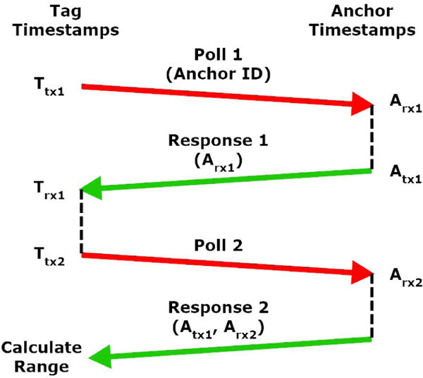
Ranging protocol between tag and anchor.
Our unsynchronized UWB approach has many distinct advantages over the synchronized anchors approach based on time difference of arrival. For example, it does not require carefully synchronized transmitters or receivers. Eliminating the need to physically interconnect the transmitters or receivers enables this technology to estimate ranges between multiple wearable sensors that are not physically connected with one another. A consequence of our unsynchronized approach is that the ranging can only be done between one pair of devices at a time, and therefore the sample rate is inversely proportional to the number of device pairs in the network.
Our proposed tightly coupled state space model includes both a nonlinear process model and a nonlinear measurement model, both with additive noise. There are a variety of algorithms available for state estimation with nonlinear state space models. The extended Kalman filter (EKF) is one of the most common for tracking pose from fused UWB and inertial sensor data. The EKF is based on linearizing the state and observation models with a first-order Taylor series expansion. If the model is highly nonlinear, then the linearization may lead to poor performance. The EKF also requires calculation of Jacobian matrices for the process and measurement models, which can be tedious and error prone.
Sequential Monte Carlo methods, also known as particle filters, can overcome the performance limitations of the EKF [23], but they have computational requirements that are orders of magnitude larger than the EKF[24, 25]. Unlike earlier approaches that used an extended Kalman filter (EKF) [21] or an iterative Kalman filter [22], we use the Unscented Kalman Filter (UKF) [26] to fuse the inertial and ranging inertial sensors. Like the EKF, it relies on a linearization of the process and measurement models, but the linearization is done statistically with sigma points, which accounts for the effects of the variability in the state estimate. The computation required by the UKF is approximately the same as the EKF, but the accuracy is typically higher. LaViola [27] has shown the UKF to be more accurate than the EKF for orientation tracking, which is a key component of pose estimation.
Previous work has not precisely quantified the accuracy of the performance in this type of applications. Consequently, it is difficult to determine from the existing literature what level of position and orientation accuracy is achievable from the fusion of these two technologies for tracking human movement. Existing work focuses on movement over a large volume, such as tracking position within a building or a large room. Our goal is to determine the feasibility of using the fused technologies to accurately estimating human movement. If successful, this may enable us to determine, for example, the feasibility of using this technology to more accurately estimate human joint angles [28, 29]. In this study, we assess the feasibility and evaluate the performance of the fused system and the algorithms through the use of an industrial robot arm with six degrees of freedom. The arm provides precise control of the movement and precise orientation and position of the inertial sensor at all times. We compare the position and orientation calculated by our tracker with those obtained from the reference system, the robot arm.
2. Methods
2.1. Instrumentation
Our instrumentation consists of a commercially available Opal inertial sensor (APDM, Inc., Portland, Oregon) and custom ranging prototyped hardware that is based on the ScenSor DWM1000 UWB ranging module (DecaWave, Inc., Dublin, Ireland), as shown in Figure 2. With further development, the inertial sensor and ranging sensors could be combined in a small, wearable device approximately the same size as the current Opal inertial sensors. In our experiments, all of the ranging sensors were stationary except for one. The stationary sensors are called anchors and the mobile sensor is called a tag. Only the tag was mechanically attached and electrically connected to the Opal inertial sensor. The anchors only included ranging hardware. All of the devices were battery powered and all control, data streaming, and communications with the devices were performed wirelessly.
Figure 2.
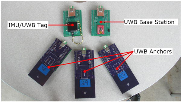
Pictures of the prototype instrumentation used for the mobile tag, stationary anchors, and base station.
The ranging sensors are controlled by a base station connected to a laptop and communicates with the tag and anchors wirelessly. To begin ranging with the set of anchors, the base station sends a trigger message to the tag. Upon receiving the trigger signal the tag conducts a ranging transaction with each anchor in sequential order. In our experiments, each ranging transaction between tag and anchor consumed 12.35 ms and was individually time-stamped and synchronized with the inertial sensor. It took the tag a total of 61.75 ms to range with all the anchors in our system. After completing ranging with all the anchors, the tag relayed the collected ranges to the base station so that they could be stored on the laptop. Storing the ranges on the laptop consumed an additional 38.25 ms. After storing the set of ranges on the laptop the base station would send a new trigger message to the tag and the entire process would repeat. This resulted in the base station sending a trigger message to the tag at a rate of 10 Hz.
2.2. State Space Model
Our proposed system uses a state space tracking framework to fuse the information from the inertial and ranging sensors, and uses the unscented Kalman filter (UKF) recursions to estimate the state of the system, which includes the position and orientation of interest. State space models include a process model that represents the prior knowledge of how the state evolves over time and a measurement model that relates the measurements to the state. If we assume additive noise, this can be represented concisely as
| (2) |
| (3) |
where n is the time index, xn is the state vector, the function fn(·) models the deterministic part of the state transition from time n to n +1, wn is a known input signal, un is additive white process noise, yn is the measurement vector, the function hn(·) models the relationship between the state and the measurements, and vn is additive white measurement noise. In our design the state vector includes the orientation, position, and velocity of the tag,
| (4) |
where qn ∈ ℝ4 is a unit quaternion representing the orientation as a rotation between the tag and the Earth frame, pn ∈ ℝ3 is the position, ṗn ∈ ℝ3 is the velocity. The input wn = [wnan]T includes the vector of gyroscope measurements ωn ∈ ℝ3 and the vector of accelerometer measurements an ∈ ℝ3.
2.3. Process Model
We use a process model based on [21],
| (5) |
| (6) |
| (7) |
where Ts is the sampling interval, ⊙ represents a quaternion product [30], R(qn) is an orthonormal 3 × 3 rotation matrix computed from the quaternion qn[30] that rotates a vector in the tag frame to the Earth frame, an is the specific force vector as measured by the accelerometer on the tag, g is a vector representing gravitational acceleration in the Earth frame,
| (8) |
and rn is a quaternion representing the change in orientation from time n to n + 1
| (9) |
where ωx,n, ωy,n, and ωz,n are the rotational rates in the tag frame as measured by the gyroscopes and
| (10) |
In practice MEMS gyroscopes and accelerometers contain noise and drift. The propose system lumps the noise components as part of the overall additive noise vector, un = [uq,nup,nuṗ,n]T The model could be easily adapted to include sensor drift as part of the state vector [21]. It is also possible to model the quaternion portion of the state vector more precisely to preserve the unit norm of the quaternion portion of the state vector [31]. The model uses a diagonal process noise covariance matrix with the standard deviations listed in Table 1.
Table 1.
Process noise standard deviations.
| Noise Term | σ |
|---|---|
| uq,k | 0.04 |
| up,k | 0.01 m |
| uṗ,k | 0.02 m/s |
2.4. Measurement Model
The proposed measurement model is the vector of Euclidean distances between the position of the tag pn and the locations of each of the stationary anchors that are known at time n,
| (11) |
where denotes the Euclidean norm, αn(i) ∈ ℝ3 is the location of the anchor, un(i) is the ith element of the measurement noise vector, Μn is the number of anchors that provided measurements at time n, and is the dimension of the measurement vector at time n.
In our instrumentation, the sample rate of the inertial sensors (128 Hz) was much higher than that of the ranging sensors (10 Hz), so during most sample times n only the measurement between the tag and a single anchor was available. However, the model is general enough to account for as many measurements as are available at time n. As a consequence, our design uses a time-varying measurement model.
We modeled the additive measurement noise as a white noise process with a diagonal covariance. The ranging sensors that we used have an error that is statistically indistinguishable from Gaussian white noise when the tag is stationary, but the error also varies with position and orientation of the tag and anchors. We combined all of these effects into the additive noise vector vn with a standard deviation of 20 cm.
3. Performance Assessment
3.1. Robotic Control of Movement
To evaluate the performance of the tracking systems, we compared the position and orientation angles calculated by the inertial tracker with those obtained from an industrial Epson C3 robot (Epson Robots, California) with six degrees of freedom, as shown in Figure 3. The arm is capable of movements that are rapid, precise, and repeatable. Although the arm was designed for industrial assembly, it is well suited for controlled studies of movement. The C3 provides angular velocities of each of the six joints in the range of 450–720°/s, has a repeatability of ±0.02 mm, and has a work area of ±48 cm × ±48 cm × ±48 cm.
Figure 3.
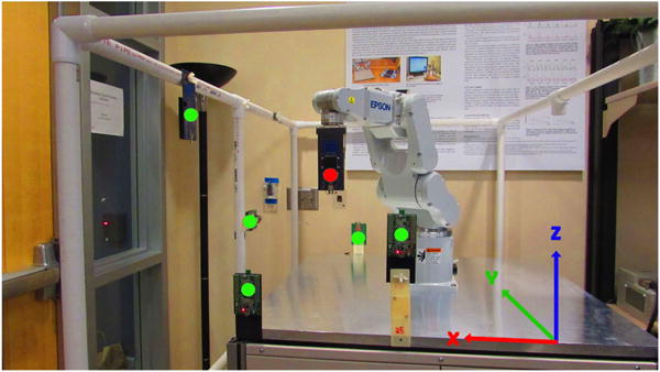
Robot (Epson C3) arm used for performance assessment.
Our tag was attached to the end effector of the Epson C3 robot. We placed five anchors around the perimeter of the robot as highlighted in green in Figure 3. The anchor placement was chosen to uniformly distribute the anchors around the tracking volume. We chose to use five anchors in order to ensure that we had enough range measurement to calculate an estimate using trilateration, however, we chose not to use more anchors so as not to reduce the sample rate on the ranging sensors. The robot frame was used as the Earth reference frame. We precisely measured the position of each anchor prior to data collection.
3.2. Sensor Calibration
To obtain the best possible performance, we performed a separate linear calibration for each tag-anchor combination. The robot was programmed to perform a linear motion from −380.0 mm to +380.0 mm in the y-axis at a speed of 10 mm/s while ranging data was recorded between the tag module and the six anchor modules. The spatial location of each anchor module was precisely measured and thus the true range between the tag module and anchor modules was known at each time sample. A linear least squares fit was used to calculate scale and offset factors for each anchor. We also estimated the bias of the gyroscopes during a brief 10 s period when the tag was held in a stationary position. The bias was subtracted from the subsequent gyroscope measurements.
3.3. Movement Protocol
To evaluate the performance of our tracker, we programmed the robot to alter the orientation and position of the tag over a range of frequencies for a sustained period of time. The movement protocol was designed to represent a range of movements, fast and slow, that are typical of human movement. We chose a 15 min total recording duration to contrast the accumulated error in orientation with inertial sensing alone with the fused estimate. The movement protocol included linear translational oscillations between ±380.0 mm along the y-axis of the Earth frame. We programmed the robot to move the tag rapidly at first and gradually decrease the speed of movement. The starting velocity and acceleration for the linear movement were set to 2.0m/s and 20.0m/s2, respectively. At either end of the linear motion, the velocity and acceleration were reduced by 0.001 m/s and 0.125 m/s2 until they reached a final value of 0.560 m/s and 2.0m/s2. The fundamental period of the movement gradually increased from 2.1 s to 8.5 s by the end of the last cycle. The orientation oscillations were over the same rates about the z-axis between ±45°. We repeated these chirp intervals of fast-to-slow movement four times with brief still periods in between each chirp interval for a total recording duration of 15 min.
3.4·Time Alignment
Although the UWB and inertial sensors were carefully synchronized through a synchronization pulse, the robot arm was not synchronized with the sensors. We accounted for both deviation from the nominal sample rates and the time offset between the two systems through a moving-window, cross-correlation analysis. The sample times of the robot arm positions and orientations were then scaled and offset to provide precise time alignment with the sensors.
3.5. Performance Criteria
We compared two different estimates of position and orientation to that of the robot, which we treated as a gold standard. Both estimates were initialized with the true position and orientation. The first estimate was obtained by fusing the range and inertial sensor measurements with an unscented Kalman filter, as described in earlier sections. Our second estimate was obtained from using the ranging sensors alone. It is not possible to estimate the orientation of the tag from these sensors. We estimated the position through trilateration, which essentially is a means of minimizing the total error,
| (12) |
where dn(i) is the measured range between the tag and the ith anchor. The trilateration is underdetermined and there are multiple solutions that produce an error of zero unless the ranges to at least four anchors are known. Since the sample rate of our estimates were chosen to match that of the inertial sensors (128 Hz) and the range measurements were only available at 10 Hz, only one range measurements were available at most sample times. To provide a continuous estimate of the position, we resampled the range measurements to 128 Hz and used the resampled range measurements to perform trilateration.
We chose to quantify the performance based on the root mean squared (RMS) error for each of the positions, x, y, and z, in the Earth frame. For example,
| (13) |
We also measured the average RMS error of the total position error. We quantified the orientation error by calculating the elevation, bank, and heading errors. This required conversion of the quaternion to Euler angles [30]. We also calculated the RMS of the total angular error, which is the angle of rotation required to rotate the estimated orientation to the true orientation.
4. Results
Table 2 summarizes the performance of the algorithm In estimating the orientation angles using the fused data from the UWB and inertial sensors. The table shows the RMS error in orientation angle estimates. Similarly, Table 3 shows the RMS error in position estimates.
Table 2.
RMS error between reference and estimated orientation angles.
| Fused | Ranging | |
|---|---|---|
| Elevation | 0.8° | – |
| Bank | 0.4° | – |
| Heading | 4.7° | – |
| Total | 4.8° | – |
Table 3.
RMS error between reference and position estimates.
| Fused | Ranging | |
|---|---|---|
| x | 2.22 cm | 2.93 cm |
| y | 3.72 cm | 3.06 cm |
| z | 2.92 cm | 6.02 cm |
| Total | 5.22 cm | 7.36 cm |
Figure 4 shows a comparison during a brief segment of the actual position (light gray) and estimated position through inertial-ranging fusion (dark red) for the y-axis. Figure 5 shows a comparison of the true heading (light gray), its estimates from the inertial-ranging fusion (dark red), and the absolute error (black in the bottom panel), during the first 270s of the recording.
Figure 4.
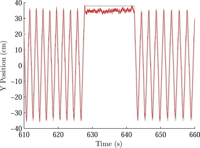
Short segment showing the true y-axis position (light gray) and the estimated position through inertial-ranging fusion (dark red).
Figure 5.
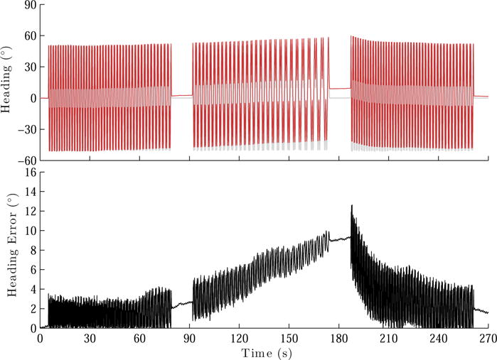
The true heading (gray), its estimate from the inertial-ranging fusion (red), and the absolute error (bottom panel) for the first 270 s of the recording.
5. Discussion
Figure 4 shows that there is a steady state error during the still period of about 5 cm between the true position and the estimate. This error is due to the ranging sensors, and is also present with the trilateration estimate based on the ranging sensors alone. This is due to a position-dependent error in the ranging sensors at this particular position. Ideally this error could be accounted for by creating a calibration for the ranging sensors that was dependent on position and orientation of the tag and the environmental conditions, but it is impractical to use this approach because it would require an extensive calibration procedure.
It is important to recognize that the fusion of the ranging and inertial sensors is only effective during movement that is sufficiently rapid. When the tag is stationary, the ranging sensors do not provide any feedback about the orientation of the tag. Similarly, when the tag is stationary the integration of the accelerometers only produces an accumulated error in the position estimate and they cannot be used to provide any information about the high frequency components of the movement. Conversely, when rapid movement is present the accelerometers can track the high frequency movements over brief periods of time. Aligning these variations in position as estimated from the accelerometers with the ranging sensors requires accurate estimation of the tag orientation. During movement with sufficiently high frequency content the UKF is able to fuse the information from the inertial sensors with the ranging sensors to perform this alignment and improve the accuracy of both the position and orientation estimates, shown in Tables 2 and 3.
Figure 5 illustrates this effect. During rapid movement near the beginning of the recording the fused estimate accurately tracks the heading. As the movement becomes slower during the period of 90–175 s, the UKF begins to lose track of the heading because the movement is slower and there is insufficient overlap in the information provided by the ranging sensors and inertial sensors to accurately determine the tag orientation. As soon as the rapid movement resumes approximately 190 s into the recording, the UKF is once again able to use the redundant information in the accelerometer and ranging sensors to estimate the tag orientation accurately.
In some respects, our experiment provides an opportunity for performance that may be more favorable than is possible in practice. As errors such as occlusion, ranging dropouts, suboptimal anchor placement, anchor position surveying errors, and calibration errors are introduced, the performance will degrade. We were careful to select a configuration of anchors that provided a position dilution of precision factor of less than 2 over the range of motion. Each tag-anchor pair was individually calibrated with a linear model from a calibration recording done prior to the experiment with the anchors in the same positions as used for the experiment. Because we were careful to avoid occlusions, we did not include a protocol for detecting and removing them, however such protocols are presented in the literature [21] and could be adapted to this model.
In other respects, it may be possible to obtain further performance improvements. For instance, it is possible to include sensor bias state variables in the state space models for the accelerometers and gyroscopes. The proposed simpler approach of subtracting the gyroscope bias as determined from a static period at the beginning of the recording and ignoring the accelerometer bias was sufficient for our purpose of determining whether the technologies could be fused to improve accuracy. However, for long duration recordings (≫ 15 min) tracking these biases may improve performance.
We also did not use gravity to improve our orientation estimates, as is common practice when working with inertial sensors alone. It is possible to estimate the elevation and bank angles during periods when the sensors are either stationary or at a constant translational velocity[15, 14]. It is also possible to use the magnetometers to estimate heading, though this is difficult in non-uniform magnetic fields[15, 14].
There is a several cm difference between the location of the inertial sensors and the location of the ranging antenna. We did not account for this because the specific movement that we used made it unnecessary. The ranging antenna is on the same axis of rotation as the inertial sensor so there is only a vertical displacement between the two sensors.
Range estimates are sensitive to antenna orientation. However, in the proposed model we did not account for this effect. It is also known that the range estimates may exhibit nonlinear distortions, particularly when the ranges are close (< 2 m), as they were in our experiment. We did not compensate for this and used a simple linear transform with only scale and bias to calibrate the range sensors.
Our tracking algorithm was causal and could easily be implemented in real time. For off line applications, smoothing methods could be used to further increase performance.
Footnotes
Publisher's Disclaimer: This is a PDF file of an unedited manuscript that has been accepted for publication. As a service to our customers we are providing this early version of the manuscript. The manuscript will undergo copyediting, typesetting, and review of the resulting proof before it is published in its final citable form. Please note that during the production process errors may be discovered which could affect the content, and all legal disclaimers that apply to the journal pertain.
References
- 1.Veltink PH, Bussman HBJ, de Vries W, Martens WLJ. Detection of static and dynamic activities using uniaxial accelerometers. IEEE Transactions on Rehabilitation Engineering. 1996;4(4):375–385. doi: 10.1109/86.547939. [DOI] [PubMed] [Google Scholar]
- 2.Chung K, El-Gohary M, Lobb B, McNames J. American Academy of Neurology 61st Annual Meeting. American Academy of Neurology; 2009. Dyskinesia estimation with inertial sensors. [Google Scholar]
- 3.El-Gohary M, McNames J, Chung K, Aboy M, Salarian A, Horak F. Proceedings of Biosignal 2010: Analysis of Biomedical Signals and Images. Vol. 20. Brno University of Technology; Brno, Czech Republic: 2010. Continuous at-home monitoring of tremor in patients with parkinson’s disease; pp. 420–424. [Google Scholar]
- 4.Spain R, St George R, Salarian A, Mancini M, Wagner J, Horak F, Bourdette D. Body-worn motion sensors detect balance and gait deficits in people with multiple sclerosis who have normal walking speed. Gait & Posture. 2012;35(4):573–578. doi: 10.1016/j.gaitpost.2011.11.026. [DOI] [PMC free article] [PubMed] [Google Scholar]
- 5.El-Gohary M, Pearson S, McNames J, Mancini M, Horak F, Mellone S, Chiari L. Continuous monitoring of turning in patients with movement disability. Sensors (Basel) 2013;14(1):356–369. doi: 10.3390/s140100356. [DOI] [PMC free article] [PubMed] [Google Scholar]
- 6.Horak F, King L, Mancini M. Role of body-worn movement monitor technology for balance and gait rehabilitation. Physical therapy. doi: 10.2522/ptj.20140253. [DOI] [PMC free article] [PubMed] [Google Scholar]
- 7.Antonsson E, Mann R. The frequency content of gait. J Biomech. 1985;18(1):39–47. doi: 10.1016/0021-9290(85)90043-0. [DOI] [PubMed] [Google Scholar]
- 8.Luinge HJ, Veltink PH. Measuring orientation of human body segments using miniature gyroscopes and accelerometers. Medical & biological engineering & computing. 2005;43(2):273–282. doi: 10.1007/BF02345966. [DOI] [PubMed] [Google Scholar]
- 9.Roetenberg D, Luinge HJ, Baten CTM, Veltink PH. Compensation of magnetic disturbances improves inertial and magnetic sensing of human body segment orientation. IEEE Transactions on Neural Systems and Rehabilitation Engineering. 2005;13(3):395–405. doi: 10.1109/TNSRE.2005.847353. [DOI] [PubMed] [Google Scholar]
- 10.Roetenberg D, Slycke PJ, Veltink PH. Ambulatory position and orientation tracking fusing magnetic and inertial sensing. IEEE Transactions on Biomedical Engineering. 2007;54(5):883–890. doi: 10.1109/TBME.2006.889184. [DOI] [PubMed] [Google Scholar]
- 11.Luinge HJ, Veltink PH, Baten CTM. Ambulatory measurement of arm orientation. Journal of Biomechanics. 2007;40:78–85. doi: 10.1016/j.jbiomech.2005.11.011. [DOI] [PubMed] [Google Scholar]
- 12.Bachmann ER, Yun X, Brumfield A. Limitation of attitude estimation algorithms for Inertial/Magnetic sensors modules. Robotics & Automation Magazine September. 2007:76–87. [Google Scholar]
- 13.Yun X, Bachmann ER, McGhee RB. A simplified quaternion-based algorithm for orientation estimation from earth gravity and magnetic field measurements. IEEE Transactions on Instrumentation and Measurement. 2008;57(3):638–650. [Google Scholar]
- 14.Sabatini AM. Estimating three-dimensional orientation of human body parts by inertial/magnetic sensing. Sensors. 2011;11(2):1489–1525. doi: 10.3390/s110201489. [DOI] [PMC free article] [PubMed] [Google Scholar]
- 15.Sabatini AM. Quaternion-based extended kalman filter for determining orientation by inertial and magnetic sensing. IEEE Transactions on Biomedical Engineering. 2006;53(7):1346–1356. doi: 10.1109/TBME.2006.875664. [DOI] [PubMed] [Google Scholar]
- 16.Zhu R, Zhou Z. A real-time articulated human motion tracking using tri-axis inertial/magnetic sensors package. IEEE Transactions on Neural Systems and Rehabilitation Engineering. 2004;12(2):295–302. doi: 10.1109/TNSRE.2004.827825. [DOI] [PubMed] [Google Scholar]
- 17.Tanigawa M, Hol JD, Dijkstra F, Luinge H, Slycke P. Augmentation of low-cost GPS/MEMS INS with UWB positioning system for seamless outdoor/indoor positioning. Proceedings of the 21st International Technical Meeting of the Satellite Division of The Institute of Navigation. 2008:1804–1811. [Google Scholar]
- 18.Zhang M, Vydhyanathan A, Young A, Luinge H. Robust height tracking by proper accounting of nonlinearities in an integrated UWB/MEMS-based-IMU/baro system. IEEE/ION. 2012 Apr 23–26 [Google Scholar]
- 19.Zwirello L, Li X, Zwick T, Ascher C, Werling S, Trommer GF. Sensor data fusion in UWB-supported inertial navigation systems for indoor navigation. IEEE ICRA. 2013 May 6–10 [Google Scholar]
- 20.Fan Q, Wu Y, Hui J, Wu L, Yu Z, Zhou L. Integrated navigation fusion strategy of INS/UWB for indoor carrier attitude angle and position synchronous tracking. The Scientific World Journal. 2014 doi: 10.1155/2014/215303. [DOI] [PMC free article] [PubMed] [Google Scholar]
- 21.Hol JD, Dijkstra F, Luinge H, Schön TB. Tightly coupled UWB/IMU pose estimation. ICUWB. 2009 [Google Scholar]
- 22.Ascher C, Werling S, Trommer GF, Zwirello L, Hansmann C, Zwick T. Radio-assisted inertial navigation system by tightly coupled sensor data fusion: Experimental results. International Conference on Indoor Positioning and Indoor Navigation. 2012 Nov 13–15; [Google Scholar]
- 23.Cappé O, Godsill S, Moulines E. An overview of existing methods and recent advances in sequential Monte Carlo. Proceedings of the IEEE. 2007;95(5):899–924. doi: 10.1109/JPR0C.2007.893250. [DOI] [Google Scholar]
- 24.Doucet A, Godsill S, Andrieu C. On sequential Monte Carlo sampling methods for Bayesian filtering. Statistics and Computing. 2000;10(3):197–208. [Google Scholar]
- 25.Djurić PM, Kotecha JH, Zhang J, Huang Y, Ghirmai T, Bugallo MF, Mìguez J. Particle filtering. IEEE Signal Processing Magazine. 2003;20(5):19–38. [Google Scholar]
- 26.Julier SJ, Uhlmann JK. Unscented filtering and nonlinear estimation. Proceedings of the IEEE. 2004;92:401–422. [Google Scholar]
- 27.L JJ., Jr A comparison of unscented and extended Kalman filtering for estimating quaternion motion. Proceedings of the 2003 American Control Conference. 2003;3:2435–2440. [Google Scholar]
- 28.El-Gohary M, McNames J. Shoulder and elbow joint angle tracking with inertial sensors. IEEE Transactions on Biomedical Engineering. 2012;59(9):577–585. doi: 10.1109/TBME.2012.2208750. [DOI] [PubMed] [Google Scholar]
- 29.El-Gohary M, McNames J. Human joint angle estimation with inertial sensors and validation with a robot arm. IEEE Transactions on Biomedical Engineering. 62(7) doi: 10.1109/TBME.2015.2403368. [DOI] [PubMed] [Google Scholar]
- 30.Kuipers JB. Quaternions and Rotation Sequences. Princeton University Press; 2002. [Google Scholar]
- 31.Kraft E. A quaternion-based unscented Kalman filter for orientation tracking. Proceedings of the Sixth International Conference of Information Fusion, 2003. 2003;1:47–54. doi: 10.1109/ICIF.2003.177425. [DOI] [Google Scholar]