High particulate iron(II) content in glacially sourced dusts enhances productivity of a model diatom

Diatoms can access mineral iron from dust if it is reduced, and reduced particulate iron is common in glacial dust sources.

Abstract

Little is known about the bioavailability of iron (Fe) in natural dusts and the impact of dust mineralogy on Fe utilization by photosynthetic organisms. Variation in the supply of bioavailable Fe to the ocean has the potential to influence the global carbon cycle by modulating primary production in the Southern Ocean. Much of the dust deposited across the Southern Ocean is sourced from South America, particularly Patagonia, where the waxing and waning of past and present glaciers generate fresh glaciogenic material that contrasts with aged and chemically weathered nonglaciogenic sediments. We show that these two potential sources of modern-day dust are mineralogically distinct, where glaciogenic dust sources contain mostly Fe(II)-rich primary silicate minerals, and nearby nonglaciogenic dust sources contain mostly Fe(III)-rich oxyhydroxide and Fe(III) silicate weathering products. In laboratory culture experiments, Phaeodactylum tricornutum, a well-studied coastal model diatom, grows more rapidly, and with higher photosynthetic efficiency, with input of glaciogenic particulates compared to that of nonglaciogenic particulates due to these differences in Fe mineralogy. Monod nutrient accessibility models fit to our data suggest that particulate Fe(II) content, rather than abiotic solubility, controls the Fe bioavailability in our Fe fertilization experiments. Thus, it is possible for this diatom to access particulate Fe in dusts by another mechanism besides uptake of unchelated Fe (Fe′) dissolved from particles into the bulk solution. If this capability is widespread in the Southern Ocean, then dusts deposited to the Southern Ocean in cold glacial periods are likely more bioavailable than those deposited in warm interglacial periods.

INTRODUCTION

High-nutrient, low-chlorophyll (HNLC) regions maintained by Fe limitation (1) span >20% of the world’s oceans (2). The Southern Ocean is the most important HNLC region in that it sets the preformed nutrient inventory of a large part of the deep ocean, which ultimately regulates the efficiency of the biological pump (3). During the latter half of the glacial cycle, modulations in the availability of dust-borne Fe and a more efficient biological pump in the subantarctic Southern Ocean appear to account for up to half of the drop in atmospheric CO₂ level associated with global cooling (4), yet we have no direct means of evaluating the relationship between productivity and particulate Fe mineralogy. Solid-phase particulate Fe is common in the ocean (5), including the Southern Ocean (6), and increasing evidence suggests that Fe particulates have varying bioavailabilities to phytoplankton based on mineralogy (6, 7). Glaciogenic Fe in Alaska that is rich in Fe(II) has been associated with high Fe solubility and is thus presumed to have high Fe bioavailability (7, 8), but new mechanisms influencing Fe bioavailability are still being discovered (9), which complicate our already-inconsistent definition of bioavailable Fe (10–14).

Measurements of Fe bioavailability in natural dusts and dust sources are generally focused on cumulative solubility estimates based on operationally defined “dissolved” Fe (7, 15), but dissolved Fe leached from natural aerosols is dominantly colloidal rather than truly soluble (15), suggesting that dust contributes readily to a particulate Fe pool that should be studied in more detail. We are interested in studying how particulate Fe mineralogy relates to Fe bioavailability to diatoms specifically. Diatoms are an important part of the carbon cycle responsible for about 40% of primary production in the modern ocean (16–19), and diatoms are an important part of the biological pump responsible for part of the atmospheric CO₂ drawdown associated with glacial periods (20). The current body of work on solid-phase Fe bioavailability to diatoms focuses just on abiotic solubility (21, 22), but recent work shows that it is possible for the cyanobacterium Trichodesmium to “mine” particulate Fe by increasing the rate of dissolution (23). Here, we probe the possibility that there is also a mechanism in diatoms that ensures that they can access particulate Fe without relying on exogenous mobilization of the Fe.

Here, we combine studies of mineralogy with direct measurements of bioavailability using natural glaciogenic dust sources and a model diatom in laboratory cultures. Iron solubility and dissociation rates generally correlate with the increased Fe bioavailability of mineralogically pure Fe colloids (24), but little has been done to probe the interactions between Fe particulates and Fe-limited phytoplankton independent of abiotically soluble Fe species or particulates dissolved biotically by bacteria (25, 26). We evaluate Fe mineralogy using x-ray absorption spectroscopy (XAS) in the fine-grained (<5 μm) fraction of nine glaciogenic and eight nonglaciogenic sediments from central and southern South America (Fig. 1 and table S1), representing potential sources of dust to the Southern Ocean (27, 28). “Glaciogenic” here describes sediments affected by glaciers during and since the last glacial period, for which weathering is dominated by physical processes. “Nonglaciogenic” describes sediments that have not been affected by glaciers in that period or longer, for which weathering is dominated by chemical processes. Although the sediment sources used in our research have relevance as potential dust sources to the subantarctic Southern Ocean (see Fig. 1, table S1, and Materials and Methods), they are mineralogically similar to and can be considered representative of glaciogenic and nonglaciogenic sediments from other locations as well (7). A subset of five mineralogically representative sediments (three glaciogenic and two nonglaciogenic, <63-μm fraction; see Materials and Methods) was used in culture experiments to directly evaluate Fe bioavailability using growth rates and cell health of the highly Fe-efficient model diatom Phaeodactylum tricornutum. Based on the relative x-ray absorption edge positions (indicative of oxidation state) in CAR19 and MK6 sediments, sediment mineralogy did not change significantly on the basis of the size fraction used (see Materials and Methods).

Fig. 1. Sample locations in South America with the right panel focused on Patagonia.

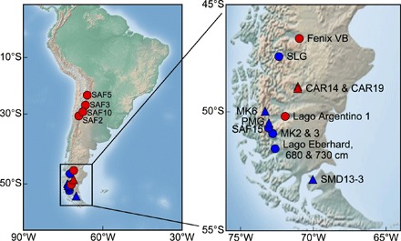
Blue and red symbols represent samples of glaciogenic and nonglaciogenic origin, respectively. Triangles indicate samples used in the culture experiments. Shaded relief image is produced with the Matplotlib Basemap Toolkit for Python. The samples are described in table S1.

After characterizing dust source mineralogy of our South American sediment samples, we examined the growth response of P. tricornutum to particulates from a subset of these sediments in laboratory culture experiments. This approach provided a way to empirically gauge the bioavailability of particulate Fe associated with our sediment samples. P. tricornutum is a well-characterized model diatom that is often used to study diatom growth under Fe limitation (29). It is a model for genotypic and evolutionary studies of diatoms (30, 31), as well as phenotypic studies applicable to open-ocean environments (17, 32, 33). Its metabolic network has also been used to frame the biogeochemical response of surface ocean systems to changing CO₂ (34).

Certainly, no single diatom species—or even a small subset of species—adequately reflects the phenotypic plasticity of marine diatoms. Iron utilization efficiency varies among diatom species and even isolates of the same species from different Fe environments (35), as well as among bloom developmental stages (36). This model diatom is coastal in origin (see Materials and Methods). Coastal diatoms, in general, have many notable physiological and evolutionary distinctions from open-ocean species, including differences in their photosynthetic systems (37, 38). However, transcriptional similarity exists among P. tricornutum and ecologically relevant diatoms, such as Thalassiosira oceanica, Fragilariopsis cylindrus, and Pseudo-nitzschia granii, in that similar Fe uptake genes are up-regulated under Fe starvation (17, 33). These understudied Fe-responsive genes in P. tricornutum are expressed in natural HNLC regions under Fe limitation (39, 40), highlighting their potential importance and the relevance of P. tricornutum as a useful model for our initial study of particulate Fe utilization.

P. tricornutum cultures were axenic (single-species; see Materials and Methods), and “no Fe added” controls (−Fe controls) and “excess Fe added” controls (+Fe controls, FeCl₃ added to 8.32 μM) were used to assess maximum achievable limitation and maximum growth rates of this organism in the growth media, respectively. We used Aquil medium with 100 μM EDTA to quickly complex solubilized Fe and ensure that the soluble bioavailable Fe (that is, unchelated Fe or Fe′) was buffered to a concentration (<0.1 pM) that is too low to support phytoplankton growth (22, 41, 42). This experimental design is intended to reduce the effect of cumulative solubility difference between the two sediment types and probe the mechanism of particulate Fe bioavailability. Monod Michaelis-Menten–type nutrient accessibility models, which will be discussed later, were used with estimates of equilibrium unchelated Fe (Fe′) (22) to show that dust-borne Fe bioavailability is not controlled by bulk [Fe′] in these experiments, although Fe′ is currently understood to be the most bioavailable form of Fe in the ocean (22).

RESULTS

Mineralogy of iron in modern natural sediments

For normalized XAS spectra (Fig. 2), the observed 2- to 3-eV shift to lower energies in the absorption edge of glaciogenic samples relative to nonglaciogenic samples indicates that the former have substantially more Fe(II)-bearing minerals than the latter (7). Both linear combination fitting (LCF) to standards and principal components analysis (PCA) revealed that ~40 to 90% of Fe in these glaciogenic sediments was Fe(II), primarily within Fe(II) silicate phases, whereas nonglaciogenic samples contained primarily Fe(III) in Fe oxyhydroxides and Fe(III) silicate phases (see tables S2 and S3 and Materials and Methods). The glaciogenic samples contained about two to four times the reduced Fe(II) content of the nonglaciogenic samples, defined as the percentage of total Fe. Our observation that there are distinct and consistent mineralogical differences between glaciogenic and nonglaciogenic sediments appears robust because the glaciogenic and nonglaciogenic sediments sampled from nearby regions in Patagonia were mineralogically different, and the nonglaciogenic sediments sampled from central South America and Patagonia were mineralogically similar, although the sampling regions are further away and geologically different from each other.

Fig. 2. XAS spectra and Fe(II) content of South American glaciogenic and nonglaciogenic sediments.

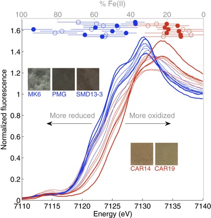
XAS spectra of all glaciogenic (blue) and nonglaciogenic (red) samples (bottom and left axes). Spectra corresponding to sediments used for culture experiments are in bold. Fe(II) content data (circles, gray top axis) are grouped as nonglaciogenic (red) and glaciogenic (blue) samples, offset for clarity. Values were calculated using PCA (open circles) and LCF (closed circles). Error bars represent SE and errors generated by the SIXPack interface (Monte Carlo simulations) for PCA and LCF fitting approaches, respectively. Images are of sediments used for culture experiments; gray color indicates reduced Fe and orange/yellow/red indicates oxidized Fe.

Bioavailability of iron in glaciogenic versus nonglaciogenic particulates

Figure 3 shows growth rate (μ), variable fluorescence (F_v/F_m), which is a photophysiological proxy for the severity of Fe limitation (43–45), and cell density for the five sediments tested plus the −Fe and +Fe controls. The diatom’s growth rate was lowest in the −Fe control, and the F_v/F_m measurements in this treatment were indicative of severe Fe limitation (44). P. tricornutum grew faster when exposed to the mineral substrates compared to the −Fe control, but the nonglaciogenic particulates were associated with less of a growth response than the glaciogenic particulates. All three indicators of Fe bioavailability were most favorable when the diatom was exposed to particulates from each of the three glaciogenic sediments. The F_v/F_m values of the diatoms exposed to glaciogenic particulates from sample SMD13-3 approached those of the Fe-replete controls here and in other Fe-rich cultures (45).

Fig. 3. Variable fluorescence (F_v/F_m), growth rates (μ), and cell densities of P. tricornutum used to evaluate particulate Fe bioavailability.

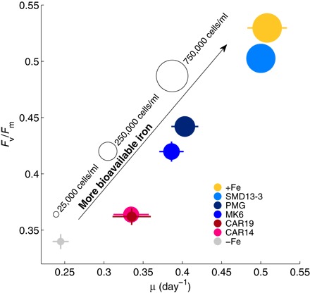
Symbol area is proportional to culture density in cells per milliliter close to the time of variable fluorescence measurement (14 days after inoculation). Variable fluorescence and cell counts were measured in triplicate. For F_v/F_m, error bars are based on the SE of 20 acquisitions per culture propagated for the triplicate cultures; for μ, error bars represent the SE of the slope of the natural log plot. Error is sometimes smaller than the symbol. Data from this experiment correspond to the circles in Fig. 4 (A to C).

Of the sediments tested, particulates from the Fe(II)-rich unweathered glaciogenic sediments uniformly supported greater diatom growth than those from the Fe(III)-dominated weathered nonglaciogenic sediments. The differences are related mainly to Fe bioavailability in the glaciogenic dust sources rather than to simply their total Fe concentrations because the glaciogenic MK6 and Perito Moreno Glacier (PMG) sediments [2.8 and 1.8 weight % (wt %) Fe, respectively] supported significantly higher growth rates compared to the nonglaciogenic CAR14 and CAR19 sediments of similar or greater Fe concentration (3.3 and 1.8 wt % Fe, respectively). The differences between the bioavailability of particulates from the nonglaciogenic CAR19 sediment and the glacial PMG sediment were particularly pronounced; despite the fact that the glaciogenic PMG has the same total Fe concentration, it produced more than four times the cell density after 14 days in culture and a significantly greater F_v/F_m ratio and growth rate than the nonglaciogenic CAR19. Glaciogenic SMD13-3 supported growth close to that of the +Fe control. Some of the enhanced growth of the cells supported by SMD13-3 compared to other particulate Fe sources is likely due to its high total Fe concentration, in addition to its high Fe(II) content [16 wt % Fe, ~40% or more of which is Fe(II); see tables S2 and S3].

Influence of iron mineralogy on particulate iron utilization

To isolate the effects of total particulate Fe concentration, [Fe′], and Fe mineralogy [particularly Fe(II) content] on the bioavailability of glaciogenic and nonglaciogenic particulates, we used the Monod Michaelis-Menten–type kinetics model for nutrient accessibility to nutrient-limited microbes (46). We plotted growth rates versus external nutrient concentrations represented as the concentration of (i) total particulate Fe added, (ii) Fe′ at equilibrium (see Materials and Methods), and (iii) particulate Fe(II) added, respectively, and fit the Monod model to each. The fits were made to the model shown in Eq. 1

$$\mathit{r}={\mathit{r}}_{\mathrm{m}}\frac{\mathit{S}}{{\mathit{K}}_{\mathit{S}}+\mathit{S}}$$ (1)

where the growth rate is expressed as the normalized growth rate r (unitless, where −Fe control represents no growth, r = 0, and +Fe control represents maximum growth, r = 1; see Materials and Methods), S is the external nutrient concentration, r_m is the normalized rate maximum under the growth conditions, and K_S is the external nutrient concentration at which the rate r is half of its maximum (r = r_m/2). In Fig. 4 (A to C), culture data are grouped by color according to whether glaciogenic (shades of blue) or nonglaciogenic (shades of red) sediment was added, and the three distinct symbol shapes indicate data from three independent experiments conducted to complete this work (that is, to achieve a range of particulate Fe concentrations, [particulate Fe], from Fe-limiting to Fe-replete conditions). All the normalized growth rates, r, are plotted against total added Fe concentrations (Fig. 4A), Fe′ (Fig. 4B), and added particulate Fe(II) concentrations (Fig. 4C), which are shown alongside the Monod kinetic models fit to the data.

Fig. 4. Monod model fits to normalized growth rates, r, as a function of three different classes of Fe species.

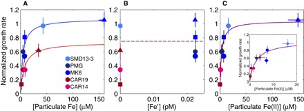
Cultures with glaciogenic sediments added are in shades of blue, and those with nonglaciogenic sediments added are in shades of red. Marker shape (circle, square, and triangle) corresponds to experiments run on three different dates. For glaciogenic particulate exposure, n = 5; for nonglaciogenic particulate exposure, n = 4. Error bars represent propagated SE for normalized rates (the same in all subplots). (A) Monod model fits (blue line is glaciogenic fit, R² = 0.82; red line is nonglaciogenic fit, R² = 0.94) as a function of total particulate Fe added to the cultures. Horizontal error bars are analytical error in particulate Fe concentration and are often smaller than the symbol size. (B) Attempted Monod fit (purple dashed line, R² = 0.22) as a function of [Fe′], with Fe′ defined as the unchelated Fe (mononuclear hydrolysis species) thought to control bioavailability of Fe in the ocean. This is an inappropriate fit because the very low K_S value implies that 3 × 10⁻¹⁹ M Fe′ can support phytoplankton growth and fully alleviate Fe limitation, which is not supported by the literature. (C) Monod model fit (purple line is the fit to all data, R² = 0.87) as a function of solid-phase Fe(II) calculated using LCF with standard spectra. The glaciogenic and nonglaciogenic data collapsing to the same curve suggest that particulate Fe(II) controls particulate Fe uptake in these cultures. Horizontal error bars are analytical error in particulate Fe(II) concentration and are often smaller than the symbol size. Inset zooms in on lower concentrations for clarity.

DISCUSSION

The fits in Fig. 4A show that Fe associated with glaciogenic sediments is a more efficient micronutrient source than Fe associated with nonglaciogenic sediments because systems modeled by Monod kinetics are driven by first-order kinetics (that is, the nutrient is limiting) below K_S and zero-order kinetics (that is, growth is independent of the nutrient concentration) above K_S. Given that K_{S(glaciogenic)} ~ 0.6 K_{S(nonglaciogenic)} (4.3 μM versus 7.4 μM), glaciogenic sediments will alleviate Fe limitation for P. tricornutum at a lower total Fe concentration than when nonglaciogenic sediments are added as the Fe source. At the lowest Fe concentrations and the ones most representative of natural growth conditions, modeled growth rates are ~2.5× higher with glaciogenic sediments versus nonglaciogenic sediments. At the highest Fe concentrations, where Fe limitation is relieved, glaciogenic particulates support ~1.5× higher growth rates than nonglaciogenic particulates (r_m of 1.07 versus 0.73).

Free bioavailable Fe concentrations [Fe′] did not significantly affect the observed experimental growth rates (Fig. 4B). This assertion is based on the combination of a poor fit of the Monod model as a function of [Fe′] (R² = 0.22) and the fact that the calculated half-saturation concentration (K_S), about 3 × 10⁻¹⁹ M, is chemically improbable. This low K_S implies that Fe limitation is alleviated for these cultures at this concentration, whereas it is well established that much higher (>0.1 pM) Fe′ concentrations are needed to support phytoplankton growth (41). Thus, both the low [Fe′] and the lack of correlation between [Fe′] and growth rate indicate that equilibrium mineral dissolution (that is, the maximum possible [Fe′] in the system) does not provide adequate Fe for growth. This result suggests that particulate Fe bioavailability to phytoplankton is driven by some mechanism besides bulk abiotic solubility alone. If growth is limited by the rate of dissolution of a mineral phase, then uptake will be a linear function of surface area (or quantity of dust). This scenario is not observed in the data. We then suggest that particulate Fe bioavailability is driven by interactions with particulate Fe(II) at the diatom-particulate interface based on our Monod model fit to all the samples when plotted against the concentration of particulate Fe(II) ([particulate Fe(II)]; Fig. 4C).

When plotting growth rates as a function of [particulate Fe(II)] in each culture (Fig. 4C), the measurements from all experiments collapse onto a single curve, indicating that [particulate Fe(II)] drives the difference in bioavailability of Fe in particulates with different mineralogy. Our observation that particulate Fe(II) is the form most accessible to our model diatom is in agreement with work that shows that synthetic Fe(III) colloids are not readily bioavailable to diatoms beyond the dissolved phase (47). On the basis of our kinetic model, Fe limitation in our cultures is alleviated at [particulate Fe(II)] above 2.7 μM. Because r_{m(glaciogenic)} slightly exceeds 1 (that is, the rate of growth in the +Fe control), we infer that highly reactive natural Fe sources are used just as efficiently, if not slightly more efficiently, by diatoms compared to the 7.3 nM Fe′ buffered by the FeEDTA complexes in our laboratory media, as calculated with Visual MINTEQ and accounting for photoreductive dissociation of FeEDTA complexes (42, 48, 49).

The utilization of particulate Fe does not preclude ligands from being important to Fe nutrition, but they cannot explain our results. Only siderophores, the strongest natural Fe ligands in the ocean, could compete with EDTA for Fe (5, 49–51). Diatoms, including P. tricornutum, do not produce their own siderophores (29, 52). Ligands existing in the culture media made from Sargasso seawater or ligands produced by any small amount of bacteria contaminating the cultures would likely affect all cultures in a similar way, suggesting that the bioavailability of particulate Fe(II) still depends on its relatively high reactivity compared to particulate Fe(III). The relatively high bioavailability of particulate Fe(II) relative to Fe(III) reflects differences in how they are obtained from the substrate. This particulate Fe utilization could entail direct accessibility of an Fe(II) substrate or could involve a microenvironment on the diatom surface where Fe is liberated and taken up before diffusion into the bulk media. In both cases, we hypothesize that surface contact between phytoplankton and particulate Fe is necessary. Some simple experiments with P. tricornutum that isolated particulate Fe in bags made from dialysis tubing provide evidence that surface contact is necessary for particulate Fe utilization by diatoms (fig. S1). Further research is required to determine the details of the mechanism by which P. tricornutum accesses particulate Fe, and these details will help us assess the global extent of particulate Fe bioavailability to diatoms. Because we used a highly studied and fully sequenced model diatom with the most advanced reverse genetics technologies (17), genetic, transcriptomic, and metatranscriptomic studies (39, 53) can be undertaken to elucidate the mechanism of Fe acquisition in detail. Other sequenced diatoms from the Southern Ocean (54) can also be studied with the same methodologies.

When evaluating the importance of more bioavailable Fe in relatively Fe(II)-rich glaciogenic particulates, it is important to consider the possible effect on the carbon cycle. In our cultures, the impact of Fe mineralogy on carbon fixation is likely greater than the observed 2.5× higher phytoplankton growth rates associated with glaciogenic particulates versus nonglaciogenic particulates because it is compounded by increases in carbon fixation rates per cell inferred from estimates of photosynthetic efficiency (F_v/F_m). Our significant increase in F_v/F_m from 0.36 to 0.5 between cultures supported by nonglaciogenic and glaciogenic particulates likely translates to about two times higher carbon fixation rates per cell on the basis of published values for P. tricornutum (29), assuming linearity between the two parameters (see Materials and Methods) (55, 56). Combined, these effects may result in about five times higher rates of carbon uptake at a constant Fe flux for glaciogenic dust versus nonglaciogenic dust fluxes to our diatoms. This estimate suggests that Fe mineralogy in natural dust sources is a critical factor in predicting how dust fluxes contribute to Fe bioavailability and CO₂ uptake by phytoplankton. Both Southern Ocean diatoms (57–60) and P. tricornutum (29) have shown increases in growth rates, decreases in Fe stress, and increases in carbon uptake in response to inputs of bioavailable Fe. More specifically, the raphid pennate lineage that includes P. tricornutum is well represented in the Southern Ocean (61, 62), and P. tricornutum can tolerate low Fe levels similar to those that sustain pennate diatoms in HNLC regions (29, 32). The results of the P. tricornutum model used here suggest that diatoms can access particulate Fe efficiently and that it is possible for additions of glaciogenic particulates to support both higher growth rates and less Fe stress in diatoms compared to nonglaciogenic particulates. Further work will delineate the phylogenetic generality of this observation, as well as the extent of the effect in natural, Fe-limited waters and the impact it has on the carbon cycle.

Our observations imply that dust sources deriving from glaciogenic sediments provide more bioavailable Fe than those deriving from nonglaciogenic materials. As such, changes over geologic time and space that affect the mineralogy of dusts to the ocean could modulate diatom growth and affect the carbon cycle. There is evidence that modern glaciogenic dust sources in Patagonia reach the subantarctic Southern Ocean within a few days (63, 64) and that any atmospheric processing would increase the fraction of particulate Fe(II) (65). Glaciogenic South American dust dominated dust supply in the Southern Hemisphere during the last glaciation (27, 28, 66–68), and these glaciogenic South American dust emissions were large (69). Because glaciogenic dust inputs to the Southern Ocean are important in the modern era and the Last Glacial Maximum (LGM), it is important that we understand how mineralogy affects Fe bioavailability and the carbon cycle both now and in the geologic past.

Our characterizations of glaciogenic and nonglaciogenic dust samples and our culture experiments with an Fe-efficient model diatom suggest that Fe mineralogy is an important factor in determining bioavailable Fe flux. Most broadly, and most significantly, we show that particulate Fe is bioavailable to diatoms independent of abiotic solubility, and the bioavailability of particulate Fe is controlled by Fe(II) mineral content. This result is in opposition to the current view that particulate Fe bioavailability depends entirely on its solubility and uptake happens through soluble phases in the bulk solution. Our results should motivate future work exploring the importance of Fe dissolution in the diffuse boundary layer of diatoms (26), as well as direct attachment of diatoms to particles. The efficiency of the global biogeochemical pump in sequestering atmospheric CO₂ by increasing nutrient consumption in the Southern Ocean is an ongoing and actively debated question (59, 60, 70), and our evaluation of the increased rate of carbon fixation with glaciogenic Fe versus nonglaciogenic Fe sources provides motivation to better constrain the effect of sediment source and mineralogy on Fe fertilization in this region. Our work shows that measuring abiotic solubility is insufficient to evaluate particulate Fe bioavailability. We report evidence that the bioavailability of dust-borne Fe to diatoms is actually much higher than previously believed because particulate Fe(II) is accessible to diatoms. Our work also suggests that Fe mineralogy in dust fluxes likely affects the Martin hypothesis of Fe limitation (1) and introduces the possibility that Fe(II) mineral content is an important predictor of particulate Fe bioavailability separate from its solubility.

MATERIALS AND METHODS

Experimental design

Here, we classified the mineralogy of Fe in natural sediments from Patagonia that represent possible dust sources to the Southern Ocean and used the same natural sediments to make direct measurements of the bioavailability of particulate Fe using laboratory experiments that involved a well-studied model diatom, P. tricornutum. We used 100 μM EDTA in the culture media to sequester unchelated Fe (Fe′) to very low (sub-0.1 pM) concentrations to probe the possibility that diatoms can access particulate Fe. Glaciogenic samples were collected primarily from southern Patagonia as the region is upwind of the Southern Ocean and the largest Patagonian glaciers exist there at present and in the past. Thus, these sediments represent the most relevant sources of dust resulting from physical weathering by glaciers that may fertilize the Southern Ocean. Our nonglaciogenic sediments are relevant in showing contrast to sediments affected by glaciers, so it was necessary that they have not been affected by glaciers during and since the last glacial period.

Sample collection and preparation

For this study, glaciogenic samples included any sediments related to glacial deposits, including moraines, till, and outwash plains, and deposited in proglacial lakes. All samples are described in table S1; the subset of three glaciogenic and two nonglaciogenic sediments used for culture experiments is further outlined here. Two of the glaciogenic samples are sediments from modern or recent glaciers, including debris coming out of the Perito Moreno Glacier (sample PMG) and the fine matrix of a moraine formed around 1970 by the modern Upsala Glacier in the Lago Argentino basin (sample MK6) (71). The third glaciogenic sample, SMD13-3, was collected from sediments laid down during the peak of the last Ice Age, about 20,000 years ago in the Strait of Magellan area (~53°S) (72); specifically, it was taken from sediments recently exposed in a gravel pit in an outwash plain, emanating from a moraine, that flowed toward and emptied into the South Atlantic Ocean. Of particular relevance in the context of our finding is the fact that SMD13-3 is directly upwind of the subantarctic sector of the Southern Ocean. This sample is also from one of the largest outwash plains in southern South America, which extended onto the continental shelf at the LGM.

The two nonglaciogenic samples, CAR14 and CAR19, were collected from Holocene-age lake deposits of Lago Cardiel, from the 55- and 45-m-level highstands, respectively (73). The Lago Cardiel basin has not been directly affected by glaciers, at least on a time period relevant to this study, and, moreover, sediments are likely derived from surrounding long-exposed and chemically weathered Mesozoic and Cenozoic sedimentary and volcanic rocks (74).

The critical sampling strategy is to work only on sediments from well-defined stratigraphic sections or landforms, so that the geologic context is well understood and, most importantly, materials of different ages and weathering processes are not mixed together in each respective sample. Five hundred to 1000 g of sediment was collected from moraines and lacustrine deposits with known sediment sources and histories. Samples were stored dry at room temperature and under atmospheric conditions until sieving to obtain the <63-μm fraction, which was carried out using ~250 ml of ultrapure water (resistivity, 18.2 megohms·cm) per ~3 to 5 g of sediment to help declump the clays. Settling, which was also carried out in ultrapure water, was used to obtain the <5-μm fraction from the <63-μm fraction. Samples were never dried in an oven but were either air- or freeze-dried within a few to several weeks of becoming wet, since the settling procedure (using Stokes’ law) took ~1 to 2 weeks in addition to the sieving process. After sorting and drying, sample preparation for XAS and culture experiments was minimal. XAS samples (<5-μm fraction) were simply spread on Kapton tape to a thickness of ~1 mm and sealed. Sediment aliquots used for cultures were sterilized with a few drops of 70% ethanol (200 proof, molecular biology grade, diluted with ultrapure water) and immediately air-dried under sterile conditions.

We used oxidation state differences defined by the difference in x-ray absorption edge position (where the normalized fluorescence spectrum crosses 0.9) between MK6 and CAR19 to show that Fe(II) estimates from the XAS analysis can be applied to the culture experiments despite using different size fractions, small differences in time the samples remained wet, and the 70% ethanol sterilization procedure for sediments used in the culture experiments. The sediments used for the culture experiments (<63 μm) had the same difference in oxidation state between the reduced glaciogenic sample (MK6) and the oxidized nonglaciogenic sample (CAR19) as the MK6 and CAR19 samples used 3 years earlier for classifying mineralogy (<5 μm). The edge position differences were 3.25 and 3.10 eV, respectively, which is well within the resolution of the instrument (0.35 to 0.8 eV). These observations suggest that the mineralogy of a sediment sample is not significantly affected by the size fraction used and that mineralogy is not affected by the ambient air long-term storage method. We attribute this stability to the fact that most of the samples were isolated from oxic environments and not susceptible to significant sample oxidation during preparation and storage. Total Fe concentrations of the <63-μm fractions used for the culture experiments were determined after wet-sieving and air-drying using x-ray fluorescence (XRF) with a Delta Innov-X handheld XRF instrument and software. Thus, any leached Fe was not erroneously included in the Fe estimates for the culture experiments. National Institute of Standards and Technology standards #2709 to #2711 were used as quality controls, with 80 to 120% recovery for Fe. Measurements were made using solid uncrushed samples to preserve them for later use in the cultures.

Synchrotron analyses

XAS at the Fe K-edge was used to probe the oxidation state and coordination environment of the Fe in the samples. Spectra with a resolution of 0.8 eV were collected on beamlines 4-1, 4-3, and 11-2 at the Stanford Synchrotron Radiation Lightsource for the dust samples and a set of mineral standards (7). The monochromator used was Si(220) at 90°, and the energy calibration was carried out using an Fe foil at 7112.0 eV (at the first inflection edge, that is, the maximum in the derivative spectrum). All spectra were collected in fluorescence mode using a 13- or 30-element Ge detector. The mineralogy of the samples was determined using LCF (7), and PCA was conducted (75, 76) primarily to group samples by oxidation state using principal components #1 and #2. To do this, principal components were determined for the sample set and then specific minerals with known compositions were fit with these principal components, after which the fraction of component #2 was regressed versus Fe(II) content to establish a linear relationship between the two (R² = 0.96); this relationship was used for each sample to determine Fe(II) content (fig. S2). Errors were reported as 67% confidence intervals based on the calibration curve. This approach is advantageous because it does not require knowledge of specific mineralogy. In contrast, LCF methods require knowledge of component minerals for accurate quantification of Fe(II), which can be difficult for some samples. However, LCF allows us to further characterize the minerals present, for example, to differentiate between Fe(II) carbonates and Fe(II) silicates or to differentiate Fe(III) in hematite from that of goethite. Pyrite, siderite, goethite, hematite, magnetite, biotite, hornblende, ferrihydrite, and glauconite standards were all used for LCF. Iron(II) content was calculated using LCF based on the oxidation state of Fe in pure minerals. We considered hornblende to contain 50% Fe(II) and 50% Fe(III). The spectra from a subset of the standards are plotted with oxidation state in fig. S3 to show similar trends in edge position and oxidation state to Fig. 2. Errors on these estimates are the errors generated by the SIXPack interface (77) propagated.

Culture experiments

The axenic P. tricornutum CCMP632 inoculate was obtained from the Provasoli-Guillard National Center for Marine Algae and Microbiota. This strain was collected from a coastal region in the British Isles, at 54°N, 4°W. Our cultures were maintained in f/2 medium, grown always at 18°C, and were kept axenic through periodic treatment with a mixture of broad-spectrum antibiotics consisting of penicillin (~2700 μg/ml), streptomycin (~540 μg/ml), and chloramphenicol (~70 μg/ml). These concentrations were optimized (78) for P. tricornutum, and the bacterial sterility of the inoculate was confirmed with periodic tests of a large aliquot of culture medium added to carbon-rich Luria-Bertani broth. Before experimentation, axenic P. tricornutum cultures were grown under Fe-limiting conditions in Aquil medium (42) with 6.7 nM added FeCl₃ and 100 μM EDTA for at least 10 generations. Aquil medium is one of the most widely used seawater media for trace metal interactions with phytoplankton (49). It uses EDTA as a trace metal buffer to control the speciation of metals in the medium. In the most recent formulation of the medium, 100 μM EDTA is used to minimize the effect of metal (in our case, Fe) contamination, including metal (Fe) impurities in the seawater and nutrients added to the cultures, or metals (Fe) introduced inadvertently during the experiment through exposure to impurities in air, etc. (32, 42, 49, 79). In our experiment, the high EDTA concentration had the added benefit of sequestering soluble Fe so we could probe the availability of particulate Fe. For our earliest experiment (triangles; Fig. 4, A to C), we relied on the time-intensive chelation step that removes the bulk of the Fe in artificial seawater and reagent-grade nutrients (42, 80). We invested in Sargasso seawater (42) and low-Fe nutrients (≥99.999% pure sodium nitrate and sodium phosphate from Fluka Analytical and sodium metasilicate containing <0.005% Fe from MP Biomedicals) for all subsequent experiments. We found it beneficial to use low-Fe EDTA as well (Sigma-Aldrich Chemistry, 99.995% trace metal basis) because reagent-grade EDTA can also contain Fe impurities. During the early experiment, artificial seawater and reagent-grade nutrients were made and chelated as outlined in the literature (42).

Cultures were grown in microwave-sterilized, acid-washed polycarbonate vials to reduce Fe contamination. An Fe-limited cell inoculate was added to ~1000 cells/ml for all cultures in all experiments. Experimental cultures were grown in filtered (acid-washed 0.2-μm Supor polyethersulfone membrane) seawater from the surface mixed layer of the Sargasso Sea that was collected in September (salinity, 36.48), except for the earliest experiment explained above. The seawater was amended to the nutrient concentrations and metal activities of Aquil with 100 μM EDTA, without added Fe. Seawater and nutrients were microwave-sterilized, and metals and vitamins were filter-sterilized before use. The temperature and light levels were maintained at 18°C and 60- to 70-μmol photons m⁻² s⁻¹ for a 12-hour light/12-hour dark cycle, respectively, for experiments as well as for maintenance cultures. A set of controls with no Fe added (−Fe) and another set with FeCl₃ added to 8.32 μM (+Fe) were grown contemporaneously with all other samples for each experiment.

Culture data were collected in three distinct experiments (circles, squares, and triangles; Fig. 4, A to C) to vary particulate Fe concentration for Monod model fits. For circles and squares, cultures were grown in 100 ml of Aquil media in acid-washed 500-ml polycarbonate bottles and were run in triplicate for each Fe source. For the experiment indicated with circles, one CAR19 culture showed evidence of significant Fe contamination and was removed from the analysis. Dust sources were added to individual bottles as 1.5 mg (circles; Fig. 4, A to C) or 2.5 mg (squares; Fig. 4, A to C) of dry sterilized sediment. For the one experiment run in quintuplicate (triangles; Fig. 4, A to C), cultures were grown in 5 ml of Aquil media in polycarbonate vials with 2.5 mg of dry sterilized sediment. We use “particulates” to refer to sediments added to culture experiments to emphasize that the diatoms were exposed to particulate Fe rather than a combination of dissolved and particulate Fe from the sediments (because EDTA complexed the soluble fraction). The <63-μm fraction of the sediment sample, separated by wet-sieving, was used to ensure that there was plenty of material for a large number of experiments. Near-edge XAS spectra of the <5-μm fraction and the <63-μm fraction of a representative subset of samples (CAR19 and MK6) showed the same oxidation state of Fe for the two fractions of the same sample, suggesting limited mineralogical differences between these fractions (see the “Sample collection and preparation” section in Materials and Methods).

Small aliquots of each culture were taken every 2 to 4 days to count cells using a hemocytometer and phase-contrast microscopy. To assess the efficiency of energy conversion by photosynthesis—that is, the maximum difference between the quantum yield of fluorescence between dark-adapted and photochemically saturated reaction centers in diatom chlorophyll—we measured variable fluorescence normalized to maximum fluorescence (F_v/F_m) in dark-adapted cells (1 hour) using a fast repetition rate fluorometer. Normalized variable fluorescence has been used extensively with P. tricornutum cultures, other single algal species, and natural seawater samples alike to assess the level of Fe limitation (44, 81). Species-specific values range from ~0.2 for the most strongly Fe-starved P. tricornutum cells to ~0.6 for the healthiest cells in the most Fe-limited and Fe-replete conditions (29, 45). Carbon uptake rates were estimated from F_v/F_m using a linear fit made to two published data points for P. tricornutum for Fe-limited and Fe-replete cells (29). This method relies on the assumption that F_v/F_m is linearly related to carbon uptake, which has been validated for natural phytoplankton assemblages (55, 56).

Linear fits to a natural log plot were used to determine the growth rate μ (equal to slope of least-squares fit) and yielded R² values of 0.97 or greater for all cultures used for both the physiology experiments (Fig. 3) and Monod curves (Fig. 4, A to C). Errors on growth rates are the SE of the regression slope. The R² values for the Monod curve fits themselves are provided in the caption of Fig. 4 (A to C). Cell counts from experimental triplicates were averaged before plotting and fitting, and plots were truncated to exclude lag and stationary phases. All fits were made to seven or eight time points for physiology experiments and to six to eight time points for Monod curves, except for the experiment indicated by triangle data points in Fig. 4 (A to C). That experiment was conducted with biological quintuplicates, and the fit was made to two data points within the exponential growth phase. Because SE of the regression slope is meaningless for a fit to two points, error was assumed to be comparable to that of the cultures from the two other experiments, and the average error from those cultures was used. This SE estimate is likely conservatively high because there were more replicates for this experiment than the others. To combine data from different experiments for the Monod curves, we normalized growth rates to a maximum rate (+Fe control) of 1 and a minimum rate (−Fe control) of 0 by subtracting the rate for the −Fe control and dividing it by the rate for the +Fe control. Errors were propagated as appropriate when rates were normalized.

Calculating [Fe′]

Estimates of soluble Fe at equilibrium were made using Visual MINTEQ (48). Aqueous components in the medium were added to the concentrations in synthetic Aquil (42). Solid species were added on the basis of the mass of sediment added to each culture, the total Fe content of the sediment, and the fraction of each mineral in the sediment. Because Fe silicates are not available in the Visual MINTEQ database, we used thermodynamic constants for minnesotaite (82), annite (83, 84), and grunerite (82) to replace those of glauconite, biotite, and hornblende, respectively, assuming congruent dissolution. It was necessary to substitute Fe silicates in these cases based on available data. The culture media were considered to be in equilibrium with CO₂ and O₂ partial pressures of 3.8 × 10⁻⁴ and 0.21 atm, respectively. The pH was fixed at 8.1 for all calculations, and the Fe²⁺/Fe³⁺ redox couple was used to account for the oxidation of Fe in the system. Ferrihydrite was allowed to precipitate. To account for photoreductive dissolution of the FeEDTA species that form in the system, the concentration of dissolved inorganic ferric hydrolysis species [Fe(III)′] was calculated using the conditional steady-state dissociation constant corrected for our 12-hour light/12-hour dark cycle and light intensity used and the concentrations of FeEDTA (FeEDTA⁻ and FeOHEDTA²⁻) and EDTA (CaEDTA²⁻ and MgEDTA²⁻) complexes at equilibrium in the media (49). Fe(II)′ was nominal in these cultures as calculated by Visual MINTEQ. For all samples, [Fe′] increased by a factor of ~4.3× when accounting for photoreductive dissociation of FeEDTA compared to [Fe′] calculated purely using Visual MINTEQ. We assumed that the system was in equilibrium with precipitated amorphous silica, but a repeated set of calculations not assuming this equilibrium yielded [Fe′] = 0.022 pM for all samples, except for the SMD13-3 sample with [Fe′] = 81 pM. The Monod kinetic model is also inappropriate using this estimate of [Fe′]. When we calculated [Fe′] in the Fe-replete Aquil medium (+Fe), we did not assume equilibrium with precipitated amorphous silica but all other parameters were the same as above. Note that our Fe silicate substitutions did not affect the modeling results because Fe(II) silicates are always unstable in oxygenated atmospheres, and they all dissolved completely in our model runs. All Fe(II) species dissolved completely in our model runs, except for the small amounts of pyrite in the glaciogenic samples, which were modeled with pyrite. Note that because these are equilibrium estimates, they are maximum [Fe′] estimates. The dissolution of Fe minerals is relatively slow. However, interactions between Fe and EDTA were relatively quick at our high EDTA concentrations (42).

Statistical analysis

To determine whether the Monod kinetics model appropriately fit the data, we used R² values and also ensured that there were no trends in the residuals.

SUPPLEMENTARY MATERIALS

Supplementary material for this article is available at http://advances.sciencemag.org/cgi/content/full/3/6/e1700314/DC1

table S1. Name, type, location, and description, with references if applicable, for each sediment sample used in this study.

table S2. LCF results for samples.

table S3. Principal component loadings.

fig. S1. Dialysis bag experiments with P. tricornutum.

fig. S2. Principal component loadings versus Fe(II) content for reference standards and samples.

fig. S3. Subset of reference spectra used for LCF that were also used for PCA, with Fe(II) content.

References (85–89)

REFERENCES AND NOTES

- 1.Martin J. H., Glacial-interglacial CO2 change: The iron hypothesis. Paleoceanography 5, 1–13 (1990). [Google Scholar]
- 2.Martin J. H., Coale K. H., Johnson K. S., Fitzwater S. E., Gordon R. M., Tanner S. J., Hunter C. N., Elrod V. A., Nowicki J. L., Coley T. L., Barber R. T., Lindley S., Watson A. J., Van Scoy K., Law C. S., Liddicoat M. I., Ling R., Stanton T., Stockel J., Collins C., Anderson A., Bidigare R., Ondrusek M., Latasa M., Millerostar F. J., Leestar K., Yao W., Zhangstar J. Z., Friederich G., Sakamoto C., Chavez F., Buck K., Kolber Z., Greene R., Falkowski P., Chisholm S. W., Hoge F., Swift R., Yungel J., Turner S., Nightingale P., Hatton A., Liss P., Tindale N. W., Testing the iron hypothesis in ecosystems of the equatorial Pacific Ocean. Nature 371, 123–129 (1994). [Google Scholar]
- 3.M. P. Hain, D. M. Sigman, G. H. Haug, The biological pump in the past, in Treatise on Geochemistry, vol. 8 (Elsevier, ed. 2, 2014), pp. 485–517. [Google Scholar]
- 4.Martínez-García A., Sigman D. M., Ren H., Anderson R. F., Straub M., Hodell D. A., Jaccard S. L., Eglinton T. I., Haug G. H., Iron fertilization of the Subantarctic Ocean during the last ice age. Science 343, 1347–1350 (2014). [DOI] [PubMed] [Google Scholar]
- 5.Boyd P. W., Ellwood M. J., The biogeochemical cycle of iron in the ocean. Nat. Geosci. 3, 675–682 (2010). [Google Scholar]
- 6.von der Heyden B. P., Roychoudhury A. N., Mtshali T. N., Tyliszczak T., Myneni S. C. B., Chemically and geographically distinct solid-phase iron pools in the southern ocean. Science 338, 1199–1201 (2012). [DOI] [PubMed] [Google Scholar]
- 7.Schroth A. W., Crusius J., Sholkovitz E. R., Bostick B. C., Iron solubility driven by speciation in dust sources to the ocean. Nat. Geosci. 2, 337–340 (2009). [Google Scholar]
- 8.Crusius J., Schroth A. W., Gassó S., Moy C. M., Levy R. C., Gatica M., Glacial flour dust storms in the Gulf of Alaska: Hydrologic and meteorological controls and their importance as a source of bioavailable iron. Geophys. Res. Lett. 38, L06602 (2011). [Google Scholar]
- 9.Tagliabue A., Bowie A. R., Boyd P. W., Buck K. N., Johnson K. S., Saito M. A., The integral role of iron in ocean biogeochemistry. Nature 543, 51–59 (2017). [DOI] [PubMed] [Google Scholar]
- 10.Mahowald N. M., Engelstaedter S., Luo C., Sealy A., Artaxo P., Benitez-Nelson C., Bonnet S., Chen Y., Chuang P. Y., Cohen D. D., Dulac F., Herut B., Johansen A. M., Kubilay N., Losno R., Maenhaut W., Paytan A., Prospero J. M., Shank L. M., Siefert R. L., Atmospheric iron deposition: Global distribution, variability, and human perturbations. Ann. Rev. Mar. Sci. 1, 245–278 (2009). [DOI] [PubMed] [Google Scholar]
- 11.Albani S., Mahowald N. M., Murphy L. N., Raiswell R., Moore J. K., Anderson R. F., McGee D., Bradtmiller L. I., Delmonte B., Hess P. P., Mayewski P. A., Paleodust variability since the Last Glacial Maximum and implications for iron inputs to the ocean. Geophys. Res. Lett. 43, 3944–3954 (2016). [Google Scholar]
- 12.Baker A. R., French M., Linge K. L., Trends in aerosol nutrient solubility along a west-east transect of the Saharan dust plume. Geophys. Res. Lett. 33, L07805 (2006). [Google Scholar]
- 13.Siefert R. L., Johansen A. M., Hoffmann M. R., Chemical characterization of ambient aerosol collected during the southwest monsoon and intermonsoon seasons over the Arabian Sea: Labile-Fe(II) and other trace metals. J. Geophys. Res. 104, 3511–3526 (1999). [Google Scholar]
- 14.Chen Y., Siefert R. L., Seasonal and spatial distributions and dry deposition fluxes of atmospheric total and labile iron over the tropical and subtropical North Atlantic Ocean. J. Geophys. Res. 109, D09305 (2004). [Google Scholar]
- 15.Aguilar-Islas A. M., Wu J., Rember R., Johansen A. M., Shank L. M., Dissolution of aerosol-derived iron in seawater: Leach solution chemistry, aerosol type, and colloidal iron fraction. Mar. Chem. 120, 25–33 (2010). [Google Scholar]
- 16.Armbrust E. V., Berges J. A., Bowler C., Green B. R., Martinez D., Putnam N. H., Zhou S., Allen A. E., Apt K. E., Bechner M., Brzezinski M. A., Chaal B. K., Chiovitti A., Davis A. K., Demarest M. S., Detter J. C., Glavina T., Goodstein D., Hadi M. Z., Hellsten U., Hildebrand M., Jenkins B. D., Jurka J., Kapitonov V. V., Kröger N., Lau W. W., Lane T. W., Larimer F. W., Lippmeier J. C., Lucas S., Medina M., Montsant A., Obornik M., Parker M. S., Palenik B., Pazour G. J., Richardson P. M., Rynearson T. A., Saito M. A., Schwartz D. C., Thamatrakoln K., Valentin K., Vardi A., Wilkerson F. P., Rokhsar D. S., The genome of the diatom Thalassiosira Pseudonana: Ecology, evolution, and metabolism. Science 306, 79–86 (2004). [DOI] [PubMed] [Google Scholar]
- 17.Tirichine L., Rastogi A., Bowler C., Recent progress in diatom genomics and epigenomics. Curr. Opin. Plant Biol. 36, 46–55 (2017). [DOI] [PubMed] [Google Scholar]
- 18.Nelson D. M., Tréguer P., Brzezinksi M. A., Leynaert A., Quéguiner B., Production and dissolution of biogenic silica in the ocean: Revised global estimates, comparison with regional data and relationship to biogenic sedimentation. Global Biogeochem. Cycles 9, 359–372 (1995). [Google Scholar]
- 19.Field C. B., Behrenfeld M. J., Randerson J. T., Falkowski P., Primary production of the biosphere: Integrating terrestrial and oceanic components. Science 281, 237–240 (1998). [DOI] [PubMed] [Google Scholar]
- 20.Brzezinksi M. A., Pride C. J., Franck V. M., Sigman D. M., Sarmiento J. L., Matsumoto K., Gruber N., Rau G. H., Coale K. H., A switch from Si(OH)4 to NO3− depletion in the glacial Southern Ocean. Geophys. Res. Lett. 29, 10.1029/2001GLO14349 (2002). [Google Scholar]
- 21.Rich H. W., Morel F. M. M., Availability of well-defined iron colloids to the marine diatom Thalassiosira weissflogii. Limnol. Oceanogr. 35, 652–662 (1990). [Google Scholar]
- 22.Lis H., Shaked Y., Kranzler C., Keren N., Morel F. M. M., Iron bioavailability to phytoplankton: An empirical approach. ISME J. 9, 1003–1013 (2015). [DOI] [PMC free article] [PubMed] [Google Scholar]
- 23.Rubin M., Berman-Frank I., Shaked Y., Dust- and mineral-iron utilization by the marine dinitrogen-fixer Trichodesmium. Nat. Geosci. 4, 529–534 (2011). [Google Scholar]
- 24.Kuma K., Matsunaga K., Availability of colloidal ferric oxides to coastal marine phytoplankton. Mar. Biol. 122, 1–11 (1995). [Google Scholar]
- 25.Boiteau R. M., Mende D. R., Hawco N. J., McIlvin M. R., Fitzsimmons J. N., Saito M. A., Sedwick P. N., DeLong E. F., Repeta D. J., Siderophore-based microbial adaptations to iron scarcity across the eastern Pacific Ocean. Proc. Natl. Acad. Sci. U.S.A. 113, 14237–14242 (2016). [DOI] [PMC free article] [PubMed] [Google Scholar]
- 26.Amin S. A., Parker M. S., Armbrust E. V., Interactions between diatoms and bacteria. Microbiol. Mol. Biol. Rev. 76, 667–684 (2012). [DOI] [PMC free article] [PubMed] [Google Scholar]
- 27.Gili S., Gaiero D. M., Goldstein S. L., Chemale F. Jr., Koester E., Jweda J., Vallelonga P., Kaplan M. R., Provenance of dust to Antarctica: A lead isotopic perspective. Geophys. Res. Lett. 43, 2291–2298 (2016). [Google Scholar]
- 28.Delmonte B., Basile-Doelsch I., Petit J.-R., Maggi V., Revel-Rolland M., Michard A., Jagoutz E., Grousset F., Comparing the EPICA and Vostok dust records during the last 220,000 years: Stratigraphical correlation and provenance in glacial periods. Earth Sci. Rev. 66, 63–87 (2004). [Google Scholar]
- 29.Allen A. E., Laroche J., Maheswari U., Lommer M., Schauer N., Lopez P. J., Finazzi G., Fernie A. R., Bowler C., Whole-cell response of the pennate diatom Phaeodactylum tricornutum to iron starvation. Proc. Natl. Acad. Sci. U.S.A. 105, 10438–10443 (2008). [DOI] [PMC free article] [PubMed] [Google Scholar]
- 30.Bowler C., Allen A. E., Badger J. H., Grimwood J., Jabbari K., Kuo A., Maheswari U., Martens C., Maumus F., Otillar R. P., Rayko E., Salamov A., Vandepoele K., Beszteri B., Gruber A., Heijde M., Katinka M., Mock T., Valentin K., Verret F., Berges J. A., Brownlee C., Cadoret J.-P., Chiovitti A., Choi C. J., Coesel S., De Martino A., Detter J. C., Durkin C., Falciatore A., Fournet J., Haruta M., Huysman M. J. J., Jenkins B. D., Jiroutova K., Jorgensen R. E., Joubert Y., Kaplan A., Kröger N., Kroth P. G., La Roche J., Lindquist E., Lommer M., Martin–Jézéquel V., Lopez P. J., Lucas S., Mangogna M., McGinnis K., Medlin L. K., Montsant A., Oudot–Le Secq M.-P., Napoli C., Obornik M., Parker M. S., Petit J.-L., Porcel B. M., Poulsen N., Robison M., Rychlewski L., Rynearson T. A., Schmutz J., Shapiro H., Siaut M., Stanley M., Sussman M. R., Taylor A. R., Vardi A., von Dassow P., Vyverman W., Willis A., Wyrwicz L. S., Rokhsar D. S., Weissenbach J., Armbrust E. V., Green B. R., Van de Peer Y., Grigoriev I. V., The Phaeodactylum genome reveals the evolutionary history of diatom genomes. Nature 456, 239–244 (2008). [DOI] [PubMed] [Google Scholar]
- 31.Oudot-Le Secq M.-P., Grimwood J., Shapiro H., Armbrust E. V., Bowler C., Green B. R., Chloroplast genomes of the diatoms Phaeodactylum tricornutum and Thalassiosira pseudonana: Comparison with other plastid genomes of the red lineage. Mol. Genet. Genomics 277, 427–439 (2007). [DOI] [PubMed] [Google Scholar]
- 32.Kustka A. B., Allen A. E., Morel F. M. M., Sequence analysis and transcriptional regulation of iron acquisition genes in two marine diatoms. J. Phycol. 43, 715–729 (2007). [Google Scholar]
- 33.Morrissey J., Sutak R., Paz-Yepes J., Tanaka A., Moustafa A., Veluchamy A., Thomas Y., Botebol H., Bouget F. Y., McQuaid J. B., Tirichine L., Allen A. E., Lesuisse E., Bowler C., A novel protein, ubiquitous in marine phytoplankton, concentrates iron at the cell surface and facilitates uptake. Curr. Biol. 25, 364–371 (2015). [DOI] [PubMed] [Google Scholar]
- 34.Levering J., Dupont C. L., Allen A. E., Palsson B. O., Zengler K., Integrated regulatory and metabolic networks of the marine diatom Phaeodactylum tricornutum predict the response to rising CO2 levels. mSystems 2, e00142-00116 (2017). [DOI] [PMC free article] [PubMed] [Google Scholar]
- 35.Marchetti A., Maldonado M. T., Lane E. S., Harrison P. J., Iron requirements of the pennate diatom Pseudo-nitzschia: Comparison of oceanic (high-nitrate, low-chlorophyll waters) and coastal species. Limnol. Oceanogr. 51, 2092–2101 (2006). [Google Scholar]
- 36.Ryan-Keogh T. J., Macey A. I., Nielsdóttir M. C., Lucas M. I., Steigenberger S. S., Stinchcombe M. C., Achterberg E. P., Bibby T. S., Moore C. M., Spatial and temporal development of phytoplankton iron stress in relation to bloom dynamics in the high-latitude North Atlantic Ocean. Limnol. Oceanogr. 58, 533–545 (2013). [Google Scholar]
- 37.Strzepek R. F., Harrison P. J., Photosynthetic architecture differs in coastal and oceanic diatoms. Nature 431, 689–692 (2004). [DOI] [PubMed] [Google Scholar]
- 38.Armbrust E. V., The life of diatoms in the world’s oceans. Nature 459, 185–192 (2009). [DOI] [PubMed] [Google Scholar]
- 39.Marchetti A., Schruth D. M., Durkin C. A., Parker M. S., Kodner R. B., Berthiaume C. T., Morales R., Allen A. E., Armbrust E. V., Comparative metatranscriptomics identifies molecular bases for the physiological responses of phytoplankton to varying iron availability. Proc. Natl. Acad. Sci. U.S.A. 109, E317–E325 (2012). [DOI] [PMC free article] [PubMed] [Google Scholar]
- 40.Chappell P. D., Whitney L. A. P., Wallace J. R., Darer A. I., Jean-Charles S., Jenkins B. D., Genetic indicators of iron limitation in wild populations of Thalassiosira oceanica from the northeast Pacific Ocean. ISME J. 9, 592–602 (2014). [DOI] [PMC free article] [PubMed] [Google Scholar]
- 41.W. G. Sunda, Bioavailability and bioaccumulation of iron in the sea, in The Biogeochemistry of Iron in Seawater, D. R. Turner, K. A. Hunter, Eds. (John Wiley & Sons, 2001). [Google Scholar]
- 42.Price N. M., Price N. M., Harrison G. I., Hering J. G., Hudson R. J., Nirel P. M. V., Palenik B., Morel F. M. M., Preparation and chemistry of the artificial algal culture medium Aquil. Biol. Oceanogr. 6, 443–461 (1989). [Google Scholar]
- 43.Behrenfeld M. J., Bale A. J., Kolber Z. S., Aiken J., Falkowski P. G., Confirmation of iron limitation of phytoplankton photosynthesis in the equatorial Pacific Ocean. Nature 383, 508–511 (1996). [Google Scholar]
- 44.Greene R. M., Geider R. J., Kolber Z., Falkowski P. G., Iron-induced changes in light harvesting and photochemical energy conversion processes in eukaryotic marine algae. Plant Physiol. 100, 565–575 (1992). [DOI] [PMC free article] [PubMed] [Google Scholar]
- 45.Geider R. J., Roche J. L., Greene R. M., Olaizola M., Response of the photosynthetic apparatus of Phaeodactylum tricornutum (Bacillariophyceae) to nitrate, phosphate, or iron starvation. J. Phycol. 29, 755–766 (1993). [Google Scholar]
- 46.Monod J., The growth of bacterial cultures. Annu. Rev. Microbiol. 3, 371–394 (1949). [Google Scholar]
- 47.Nodwell L. M., Price N. M., Direct use of inorganic colloidal iron by marine mixotrophic phytoplankton. Limnol. Oceanogr. 46, 765–777 (2001). [Google Scholar]
- 48.J. P. Gustafsson, Visual MINTEQ, ver. 3.1 (2016).
- 49.W. G. Sunda, N. M. Price, F. M. M. Morel, Trace metal ion buffers and their use in culture studies, in Algal Culturing Techniques, R. A. Anderson, Ed. (Elsevier Academic Press, 2005), pp. 35–63. [Google Scholar]
- 50.Mawji E., Gledhill M., Milton J. A., Tarran G. A., Ussher S., Thompson A., Wolff G. A., Worsfold P. J., Achterberg E. P., Hydroxamate siderophores: Occurrence and importance in the Atlantic Ocean. Environ. Sci. Technol. 42, 8675–8680 (2008). [DOI] [PubMed] [Google Scholar]
- 51.Wu J., Boyle E., Sunda W., Wen L.-S., Soluble and colloidal iron in the oligotrophic North Atlantic. Science 293, 847–849 (2001). [DOI] [PubMed] [Google Scholar]
- 52.Hopkinson B. M., Morel F. M. M., The role of siderophores in iron acquisition by photosynthetic marine microorganisms. Biometals 22, 659–669 (2009). [DOI] [PubMed] [Google Scholar]
- 53.Pearson G. A., Lago-Leston A., Cánovas F., Cox C. J., Verret F., Lasternas S., Duarte C. M., Agusti S., Serrão E. A., Metatranscriptomes reveal functional variation in diatom communities from the Antarctic Peninsula. ISME J. 9, 2275–2289 (2015). [DOI] [PMC free article] [PubMed] [Google Scholar]
- 54.Mock T., Otillar R. P., Strauss J., McMullan M., Paajanen P., Schmutz J., Salamov A., Sanges R., Toseland A., Ward B. J., Allen A. E., Dupont C. L., Frickenhaus S., Maumus F., Veluchamy A., Wu T., Barry K. W., Falciatore A., Ferrante M. I., Fortunato A. E., Glöckner G., Gruber A., Hipkin R., Janech M. G., Kroth P. G., Leese F., Lindquist E. A., Lyon B. R., Martin J., Mayer C., Parker M., Quesneville H., Raymond J. A., Uhlig C., Valas R. E., Valentin K. U., Worden A. Z., Armbrust E. V., Clark M. D., Bowler C., Green B. R., Moulton V., van Oosterhout C., Grigoriev I. V., Evolutionary genomics of the cold-adapted diatom Fragilariopsis cylindrus. Nature 541, 536–540 (2017). [DOI] [PubMed] [Google Scholar]
- 55.Kolber Z., Falkowski P. G., Use of active fluorescence to estimate phytoplankton photosynthesis in situ. Limnol. Oceanogr. 38, 1646–1665 (1993). [Google Scholar]
- 56.Corno G., Letelier R. M., Abbott M. R., Karl D. M., Assessing primary production variability in the North Pacific Subtropical Gyre: A comparison of fast repetition rate fluorometry and 14C measurements. J. Phycol. 42, 51–60 (2005). [Google Scholar]
- 57.Strzepek R. F., Hunter K. A., Frew R. D., Harrison P. J., Boyd P. W., Iron-light interactions differ in Southern Ocean phytoplankton. Limnol. Oceanogr. 57, 1182–1200 (2012). [Google Scholar]
- 58.Hoppe C. J. M., Hassler C. S., Payne C. D., Tortell P. D., Rost B., Trimborn S., Iron limitation modulates ocean acidification effects on Southern Ocean phytoplankton communities. PLOS ONE 8, e79890 (2013). [DOI] [PMC free article] [PubMed] [Google Scholar]
- 59.Boyd P., Watson A. J., Law C. S., Abraham E. R., Trull T., Murdoch R., Bakker D. C. E., Bowie A. R., Buesseler K. O., Chang H., Charette M., Croot P., Downing K., Frew R., Gall M., Hadfield M., Hall J., Harvey M., Jameson G., LaRoche J., Liddicoat M., Ling R., Maldonado M. T., McKay R. M., Nodder S., Pickmere S., Pridmore R., Rintoul S., Safi K., Sutton P., Strzepek R., Tanneberger K., Turner S., Waite A., Zeldis J., A mesoscale phytoplankton bloom in the polar Southern Ocean stimulated by iron fertilization. Nature 407, 695–702 (2000). [DOI] [PubMed] [Google Scholar]
- 60.Smetacek V., Klaas C., Strass V. H., Assmy P., Montresor M., Cisewski B., Savoye N., Webb A., d’Ovidio F., Arrieta J. M., Bathmann U., Bellerby R., Berg G. M., Croot P., Gonzalez S., Henjes J., Herndl G. J., Hoffmann L. J., Leach H., Losch M., Mills M. M., Neill C., Peeken I., Röttgers R., Sachs O., Sauter E., Schmidt M. M., Schwarz J., Terbrüggen A., Wolf-Gladrow D., Deep carbon export from a Southern Ocean iron-fertilized diatom bloom. Nature 487, 313–319 (2012). [DOI] [PubMed] [Google Scholar]
- 61.Green S. E., Sambrotto R. N., Plankton community structure and export of C, N, P and Si in the Antarctic Circumpolar Current. Deep Sea Res. Pt. II 53, 620–643 (2006). [Google Scholar]
- 62.Hinz D. J., Nielsdóttir M. C., Korb R. E., Whitehouseb M. J., Poulton A. J., Moore C. M., Achterberg E. P., Bibby T. S., Responses of microplankton community structure to iron addition in the Scotia Sea. Deep Sea Res. Pt. II 59-60, 36–46 (2012). [Google Scholar]
- 63.Gassó S., Stein A. F., Does dust from Patagonia reach the sub-Antarctic Atlantic Ocean? Geophys. Res. Lett. 34, L01801 (2007). [Google Scholar]
- 64.Neff P. D., Bertler N. A. N., Trajectory modeling of modern dust transport to the Southern Ocean and Antarctica. J. Geophys. Res. Atmos. 120, 9303–9322 (2015). [Google Scholar]
- 65.Longo A. F., Feng Y., Lai B., Landing W. M., Shelley R. U., Nenes A., Mihalopoulos N., Violaki K., Ingall E. D., Influence of atmospheric processes on the solubility and composition of iron in Saharan dust. Environ. Sci. Technol. 50, 6912–6920 (2016). [DOI] [PubMed] [Google Scholar]
- 66.Sugden D. E., McCulloch R. D., Bory A. J.-M., Hein A. S., Influence of Patagonian glaciers on Antarctic dust deposition during the last glacial period. Nat. Geosci. 2, 281–285 (2009). [Google Scholar]
- 67.Basile I., Grousset F. W., Revel M., Petit J. R., Biscaya P. E., Barkov N. I., Patagonian origin of glacial dust deposited in East Antarctica (Vostok and Dome C) during glacial stages 2, 4, and 6. Earth Planet. Sci. Lett. 146, 573–589 (1997). [Google Scholar]
- 68.Gaiero D. M., Brunet F., Probst J.-L., Depetris P. J., A uniform isotopic and chemical signature of dust exported from Patagonia: Rock sources and occurrence in southern environments. Chem. Geol. 238, 107–120 (2007). [Google Scholar]
- 69.Mahowald N. M., Muhs D. R., Levis S., Rasch P. J., Yoshioka M., Zender C. S., Luo C., Change in atmospheric mineral aerosols in response to climate: Last glacial period, preindustrial, modern, and doubled carbon dioxide climates. J. Geophys. Res. 111, D10202 (2006). [Google Scholar]
- 70.Lampitt R. S., Bett B. J, Kiriakoulakis K., Popova E. E., Ragueneau O., Vangriesheim A., Wolff G. A., Material supply to the abyssal seafloor in the Northeast Atlantic. Prog. Oceanogr. 50, 27–63 (2001). [Google Scholar]
- 71.Strelin J. A., Kaplan M. A., Vandergoes M. J., Denton G. H., Schaefer J. M., Holocene glacier history of the Lago Argentino basin, Southern Patagonian Icefield. Quat. Sci. Rev. 101, 124–145 (2014). [Google Scholar]
- 72.Kaplan M. R., Fogwill C. J., Sugden D. E., Hulton N. R. J., Kubik P. W., Freeman S. P. H. T., Southern Patagonian glacial chronology for the Last Glacial period and implications for Southern Ocean climate. Quat. Sci. Rev. 27, 284–294 (2008). [Google Scholar]
- 73.Stine S., Stine M., A record from Lake Cardiel of climate change in southern South America. Nature 345, 705–708 (1990). [Google Scholar]
- 74.Ramos V. A., Geología de la región del lago Cardiel, provincia de Santa Cruz. Rev. Asoc. Geol. Argent. 37, 23–49 (1982). [Google Scholar]
- 75.Ressler T., Wong J., Roos J., Smith I. L., Quantitative speciation of Mn-bearing particulates emitted from autos burning (methylcyclopentadienyl)manganese tricarbonyl-added gasolines using XANES spectroscopy. Environ. Sci. Technol. 34, 950–958 (2000). [Google Scholar]
- 76.Scheinost A. C., Kretzschmar R., Pfister S., Combining selective sequential extractions, x-ray absorption spectroscopy, and principal component analysis for quantitative zinc speciation in soil. Environ. Sci. Technol. 36, 5021–5028 (2002). [DOI] [PubMed] [Google Scholar]
- 77.Webb S. M., SIXPack: A graphical user interface for XAS analysis using IFEFFIT. Phys. Scr. T115, 1011–1014 (2005). [Google Scholar]
- 78.Droop M. R., A procedure for routine purification of algal cultures with antibiotics. Br. Phycol. Bull. 3, 295–297 (1967). [Google Scholar]
- 79.Hudson R. J. M., Morel F. M. M., Iron transport in marine phytoplankton: Kinetics of cellular and medium coordination reactions. Limnol. Oceanogr. 35, 1002–1020 (1990). [Google Scholar]
- 80.Morel F. M. M., Reuter J. G., Anderson D. M., Guillard R. R. L., Aquil: A chemically defined phytoplankton culture medium for trace metal studies. J. Phycol. 15, 135–141 (1979). [Google Scholar]
- 81.Greene R. M., Geider R. J., Falkowsski P. G., Effect of iron limitation on photosynthesis in a marine diatom. Limnol. Oceanogr. 36, 1772–1782 (1991). [Google Scholar]
- 82.G. Faure, Principles and Applications of Geochemistry (Prentice Hall, 1998). [Google Scholar]
- 83.Dachs E., Benisek A., Standard-state thermodynamic properties of annite, KFe3[(OH)2AlSi3O10], based on new calorimetric measurements. Eur. J. Mineral. 27, 603–616 (2015). [Google Scholar]
- 84.Zen E., An oxygen buffer for some peraluminous granites and metamorphic rocks. Am. Mineral. 70, 65–73 (1985). [Google Scholar]
- 85.Sagredo E. A., Moreno P. I., Villa-Martinez R., Kaplan M. R., Kubik P. W., Stern C. R., Fluctuations of the Ultima Esperanza ice lobe (52 degrees S), Chilean Patagonia, during the last glacial maximum and termination 1. Geomorphology 125, 92–108 (2011). [Google Scholar]
- 86.Garcia J.-L., Hall B. L., Kaplan M. R., Vega R. M., Strelin J. A., Glacial geomorphology of the Torres del Paine region (southern Patagonia): Implications for glaciation, deglaciation, and paleolake history. Geomorphology 204, 599–616 (2014). [Google Scholar]
- 87.Kaplan M. R., Schaefer J. M., Strelin J. A., Denton G. H., Anderson R. F., Vandergoes M. J., Finkel R. C., Schwartz R., Travis S. G., Garcia J. L., Martini M. A., Nielsen S. H. H., Patagonian and southern South Atlantic view of Holocene climate. Quat. Sci. Rev. 141, 112–125 (2016). [Google Scholar]
- 88.Bockheim J. G., Douglass D. C., Origin and significance of calcium carbonate in soils of southwestern Patagonia. Geoderma 136, 751–762 (2006). [Google Scholar]
- 89.McGee D., Winckler G., Borunda A., Serno S., Anderson R. F., Recasens C., Bory A., Gaiero D., Jaccard S. L., Kaplan M., McManus J. F., Tracking eolian dust with helium and thorium: Impacts of grain size and provenance. Geochim. Cosmochim. Acta 175, 47–67 (2016). [Google Scholar]
Associated Data
This section collects any data citations, data availability statements, or supplementary materials included in this article.