Abstract
Speech separation can be formulated as learning to estimate a time-frequency mask from acoustic features extracted from noisy speech. For supervised speech separation, generalization to unseen noises and unseen speakers is a critical issue. Although deep neural networks (DNNs) have been successful in noise-independent speech separation, DNNs are limited in modeling a large number of speakers. To improve speaker generalization, a separation model based on long short-term memory (LSTM) is proposed, which naturally accounts for temporal dynamics of speech. Systematic evaluation shows that the proposed model substantially outperforms a DNN-based model on unseen speakers and unseen noises in terms of objective speech intelligibility. Analyzing LSTM internal representations reveals that LSTM captures long-term speech contexts. It is also found that the LSTM model is more advantageous for low-latency speech separation and it, without future frames, performs better than the DNN model with future frames. The proposed model represents an effective approach for speaker- and noise-independent speech separation.
I. INTRODUCTION
Speech separation is the task of separating target speech from background noise. It has many applications, such as hearing aids and robust automatic speech recognition (ASR). Speech separation at low signal-to-noise ratios (SNRs) is very challenging, especially from single-microphone recordings. The task can be formulated as a supervised learning problem where a time-frequency (T-F) mask is estimated from noisy speech. A T-F mask preserves speech-dominant parts and suppresses noise-dominant parts in a T-F representation of noisy speech. Unlike speech enhancement (Ephraim and Malah, 1984; Erkelens et al., 2007; Loizou, 2013), supervised separation does not make assumptions about the statistical distribution of underlying speech or noise signals, and represents a data-driven strategy to deal with background noises.
Supervised separation typically learns a mapping from acoustic features of noisy speech to a masking function. The ideal binary mask (IBM), which labels a T-F unit as either speech-dominant or noise-dominant, is a commonly used masking function (Wang, 2005). Alternatively, a soft label on a T-F unit leads to the definition of the ideal ratio mask (IRM) (Srinivasan et al., 2006; Wang et al., 2014; Hummersone et al., 2014):
| (1) |
where and denote speech energy and noise energy within a T-F unit at time t and frequency f, respectively. A recent study has shown that ratio masking leads to better speech quality than binary masking (Wang et al., 2014). Deep neural networks (DNNs) have been very successful in supervised separation (Wang and Wang, 2013; Xu et al., 2014; Huang et al., 2015). Recent listening tests demonstrate that IRM estimation using a DNN substantially improves speech intelligibility of hearing-impaired and normal hearing listeners (Healy et al., 2013; Chen et al., 2016b). In this study, we use the IRM as the learning target of supervised separation.
For supervised learning tasks, generalizing to unseen conditions is a critical issue. Noise generalization and speaker generalization are two important aspects for supervised speech separation. The first aspect has been investigated in recent studies. With noise expansion through frequency perturbation, a model trained on one noisy type performs well with unseen segments of the same noise type (Chen et al., 2016a; Healy et al., 2015). A DNN-based IRM estimator, when trained with a large variety of noises but a fixed speaker, generalizes to unseen noises and unseen SNRs, and leads to clear speech intelligibility improvement (Chen et al., 2016b). However, it remains unknown how well such a model generalizes to unseen speakers and unseen noises at the same time.
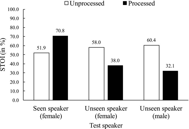
In this study, we investigate speaker generalization of noise-independent models. To illustrate the problem, we first evaluate a speaker-dependent DNN on both seen and unseen speakers. A five-hidden-layer DNN is trained on 320 000 mixtures created using 67 utterances of a female speaker and 10 000 noises. A test set is created from another 25 utterances of the same female speaker and an unseen babble noise at −5 dB SNR. Then, we create another two test sets with an unseen female speaker and an unseen male speaker. Figure 1 shows the performance of the speaker-dependent DNN on seen and unseen speakers in terms of the short-time objective intelligibility (STOI) score (Taal et al., 2011), which compares the envelopes of separated speech and clean speech and computes a score between 0% and 100%. A higher STOI score indicates higher objective speech intelligibility. As expected, the speaker-dependent DNN significantly improves STOI for the seen speaker. However, for both unseen speakers, the STOI scores of processed speech do not improve over those of unprocessed speech; they are actually lower. A DNN trained on a single speaker seems incapable of separating a new speaker from background noise.
FIG. 1.
Performance of a speaker-dependent DNN on seen and unseen speakers with a babble noise in terms of STOI (in %) at −5 dB SNR.
A straightforward approach for speaker generalization is to train a DNN-based IRM estimator on a large number of speakers and noises. Our experiments (see Sec. IV) indicate that, unfortunately, a DNN does not appear to have the capacity of modeling many speakers. Even with a large number of training speakers, a DNN still performs rather poorly on unseen speakers. A recent study (Kolbæk et al., 2017) also shows performance degradation of a speaker-generic model compared to a speaker-specific model. A less challenging setting, which we call speaker-set-dependent, is to train a model with a closed set of speakers and test it on the same speakers. Our experimental results show that the performance of a speaker-set-dependent DNN on seen speakers degrades as the number of training speakers increases. Unlike a DNN trained on a single speaker, a speaker-set-dependent DNN is exposed to many speakers during training and therefore learns to detect speech patterns for many different speakers. While a speaker-dependent DNN focuses on separating one speaker from background noise, a set-dependent DNN has to search for many potential speakers. When the background noise contains speech components (e.g., babble noise), a speaker-set-dependent DNN is likely to mistake interfering speech for target speech since the patterns of interfering speech may resemble those of some training speakers.
A strategy to resolve the confusability of target speech and noise is for a speaker-set-dependent model to detect and focus on a target speaker. One such method is to train many speaker-dependent models and use speaker identification for model selection. However, this method has several potential limitations. First, the performance on seen speakers depends on the accuracy of speaker identification, which is known to be challenging in noisy environments (Zhao et al., 2014). Second, it is limited to the closed set of trained speakers; For an unseen speaker, it needs to find a way to align the speaker to a similar trained speaker, which can also be difficult. A related method based on non-negative matrix factorization (NMF) learns a dictionary for each training speaker, and identifies a few speakers to approximate an unseen speaker during testing (Sun and Mysore, 2013). However, selecting appropriate speaker dictionaries can be challenging with nonstationary noises.
A supervised mask estimator typically uses a window of consecutive time frames to extract features to provide a useful context for improved mask estimation at a current frame. In other words, each mask frame is estimated independently given a context window containing limited temporal information about a target speaker. However, even with a long context window, the information beyond the window is not utilized. Mask estimation at a current frame can potentially benefit if a model utilizes earlier observations to characterize the target speaker. Therefore, supervised speech separation may be better formulated as a sequence-to-sequence mapping where a sequence of mask frames is predicted from a sequence of acoustic features.
In this study, we propose a model to separate unseen speakers from unseen noises. Our model is based on a recurrent neural network (RNN) and accounts for temporal dynamics of speech. An RNN has self connections to feed back previous hidden activations, unlike a DNN which is a feedforward network. For a multilayer RNN, both low-level and high-level features of the previous time step are carried forward to facilitate learning of long-term dependencies. Given an incoming stream of noisy speech, our model analyzes and separates a target speaker from noise. The model learns from previous frames to focus on the target speaker for better speaker generalization. This paper is organized as follows. Section II describes the proposed model in detail. Experimental setup is discussed in Sec. III. We present and analyze experimental results in Sec. IV. Section V concludes the paper. A preliminary version of this paper is included in Chen and Wang (2016).
II. SYSTEM DESCRIPTION
For speaker-independent speech separation, effectively modeling a target speaker is crucial. Given that characterizing a target speaker likely requires long-term observations, we propose to use RNNs to account for temporal dynamics of speech. A traditional DNN-based model only utilizes a window of features to capture temporal dynamics, which appears insufficient for speaker characterization for the sake of speech separation. In contrast, an RNN makes each mask prediction using information extracted from many previous frames.
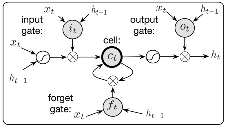
To model temporal dependencies, an RNN is typically trained with back propagation through time (BPTT). A standard RNN suffers from the exploding and vanishing gradients during BPTT (Bengio et al., 1994; Pascanu et al., 2013). While the exploding gradient problem can be mitigated using gradient clipping, the vanishing gradient problem prematurely stops an RNN from learning long-term dependencies. Long short-term memory (LSTM) (Hochreiter and Schmidhuber, 1997), a variant of RNN, mitigates the vanishing gradient problem by introducing a memory cell that facilitates the information flow over time. LSTM has been successful in modeling long temporal dependencies in many recent applications such as language modeling (Sutskever et al., 2014; Sundermeyer et al., 2015), acoustic modeling (Graves et al., 2013; Sak et al., 2014) and video classification (Ng et al., 2015). While recent studies explored LSTM for speech enhancement (Weninger et al., 2015; Erdogan et al., 2015), our study focuses on speaker- and noise-independent speech separation. Figure 2 shows an LSTM block, which depicts a memory cell and three gates where the forget gate controls how much previous information should be erased from the cell and the input gate controls how much information should be added to the cell. In this study, we use LSTM defined by the following equations (Gers et al., 2000):
| (2) |
| (3) |
| (4) |
| (5) |
| (6) |
| (7) |
| (8) |
| (9) |
where xt, zt, ct, ht represent input, block input, memory cell and hidden activation at time t, respectively. Input gate, forget gate and output gate are denoted as it, ft, and ot, respectively. W's and b's denote weights and biases, respectively. Represents element-wise multiplication or the gating operation. While the three gates are bounded to by the function , the output of an LSTM block is bounded to by both and g(s). Note that the input gate it and the forget gate ft are dependent on the current lower-layer input xt and the previous hidden activation . This dependency makes the updating of the memory cell context-sensitive, and therefore enables the modeling of complex temporal dynamics. With training by BPTT, LSTM supposedly learns to store task-relevant and context-sensitive information in its memory cells.
FIG. 2.
Diagram of an LSTM block with three gates and a memory cell.
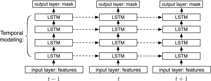
In supervised speech separation, we trained LSTM to maintain the speaker-sensitive information extracted from many previous frames to improve mask estimation for a current frame. The proposed system is illustrated in Fig. 3. We use four stacked hidden LSTM layers for temporal modeling and one output layer for mask estimation. We describe the system using the following equations:
| (10) |
| (11) |
| (12) |
where ft denotes acoustic features at time t. and represent the input and output of the LSTM block at layer l and time t, respectively. The estimated mask at time t is denoted as yt. Wout and bout represent the weight and bias of the output layer, respectively. While the bottom LSTM layer directly receives acoustic features, the other LSTM layers take the hidden activation from the LSTM layer below. The output layer takes the hidden activation , L = 4, of the top LSTM layer, and estimates the IRM.
FIG. 3.
Diagram of the proposed system. Four stacked LSTM layers are used to model temporal dynamics of speech. Three time steps are shown here.
As shown in Fig. 3, compared to a DNN-based system which only passes information from the input layer to the output layer successively, an LSTM-based system adds multiple information pathways in the time dimension, where different pathways carry forward features at different levels of abstraction.
In this study, we use a feature window of 23 frames (11 to the left, 11 to the right) to estimate one frame of the IRM, which is defined on a 64-channel cochleagram with a 20-ms frame length and a 10-ms frame shift (Wang and Brown, 2006). The estimated IRM is used to weight subband signals from a 64-channel gammatone filterbank. The weighted subband signals are summed to derive separated speech. The input features are 64-dimensional gammatone filterbank energies (Chen et al., 2016b) extracted from noisy speech. From the input layer to the output layer, the proposed network has 23 × 64, 1024, 1024, 1024, 1024, and 64 units, respectively. In our evaluations, we compare the proposed RNN with a DNN baseline, which has five hidden layers with rectified linear units (ReLUs) (Nair and Hinton, 2010) and one sigmoidal output layer. From the input layer to the output layer, the DNN has 23 × 64, 2048, 2048, 2048, 2048, 2048, and 64 units, respectively. Compared to the LSTM, this DNN is deeper and wider aside from no recurrent connections, and it provides a strong baseline.
III. EXPERIMENTAL SETUP
A. Data preparation
We create large training sets with different numbers of training speakers to investigate speaker generalization of noise-independent LSTMs and DNNs. The trained models are tested on six seen speakers and six unseen speakers, both with unseen noises. Testing on multiple seen speakers is expected to be less challenging than testing on unseen speakers, and it serves as an intermediate step towards to speaker generalization.
In our experiments, we use 7138 utterances (83 speakers, about 86 utterances per speaker) from the WSJ0 SI-84 training set (Paul and Baker, 1992), which is widely used for speech separation and recognition evaluation. To create noisy speech, we use 10 000 training noises from a sound effect library (available at http://www.sound-ideas.com), and two highly nonstationary test noises (babble and cafeteria) from an Auditec CD (available at http://www.auditec.com). Among the 83 speakers, all utterances of the six unseen speakers and the test utterances of six seen speakers are excluded from training. Since we investigate speaker generalization of noise-independent models, the two test noises are never used during training. We create the following two test sets:
-
•
Test Set 1: 150 mixtures are created from 25 × 6 utterances of six seen speakers (three males and three females) and random segments of the babble noise at −5 dB SNR.
-
•
Test Set 2: 150 mixtures are created from 25 × 6 utterances of six unseen speakers (three males and three females) and random segments of the babble noise at −5 dB SNR.
We create each training mixture by mixing an utterance with a random segment drawn from the 10 000 noises at a random SNR drawn from {−5, −4, −3, −2, −1, 0} dB. To investigate the impact of the number of training speakers on speaker generalization, we evaluate three categories of models:
-
•
Speaker-dependent models:
For each speaker in Test Set 1 and Test Set 2, we train and test on the same speaker. Each training set has 320 000 mixtures and the total duration is about 500 h.
-
•
Speaker-set-dependent model:
Five models are trained with {6, 10, 20, 40, 77} speakers including the six speakers of Test Set 1 and evaluated with Test Set 1. Each training set has 3 200 000 mixtures (about 5000 h).
-
•
Speaker-independent models:
Five models are trained with {6, 10, 20, 40, 77} speakers and tested on the six unseen speakers of Test Set 2. Each training set includes 3 200 000 mixtures (about 5000 h).
B. Optimization methods
We train the DNN and LSTM with the mean square error (MSE) cost function and the Adam optimizer (Kingma and Ba, 2015) whose adaptive learning rates lead to faster convergence than standard stochastic gradient descent. The initial global learning rate is set to 0.001 and reduced by half every epoch. The best model is selected by cross validation. We use a mini-batch size of 256 for speaker-dependent DNNs. A mini-batch size of 4096 is used for speaker-set-dependent DNNs as we find a larger batch size slightly improves optimization. All LSTMs are trained with a mini-batch size of 256 and with truncated BPTT (Williams and Peng, 1990) of 250 time steps. For all LSTMs, we add 1 to the bias in Eq. (5) to facilitate gradient flow and encourage learning of long-term dependencies in the beginning of training (Jozefowicz et al., 2015):
| (13) |
IV. EXPERIMENTAL RESULTS AND ANALYSIS
To evaluate the generalizability of the DNN and LSTM, we use three metrics including the MSE of the estimated mask, STOI and HIT–FA rate (Kim et al., 2009). The latter compares an estimated binary mask with the IBM. HIT refers the percentage of correctly classified speech-dominant T-F units, and FA refers to false alarm or the percentage of wrongly classified noise-dominant T-F units. Since we use the IRM as the learning target, we binarize it to compute HIT–FA. During binarization, the local criterion (LC) in the IBM definition is set to be 5 dB lower than the test SNR. Both the STOI and HIT–FA rate have been shown to correlate with human speech intelligibility well (Healy et al., 2013; Kim et al., 2009).
A. Performance trend on seen test speakers
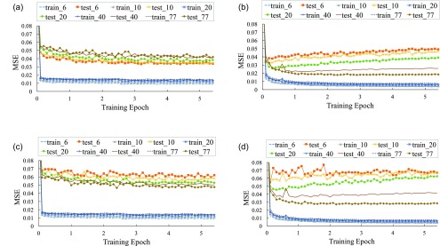
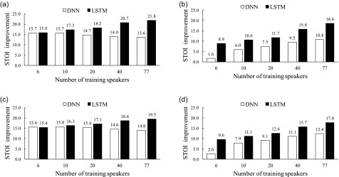
We evaluate the DNN and LSTM with six seen speakers. First, we train with the same six speakers. Figure 4 compares the training and test errors of the DNN and LSTM over training epochs. Figure 4(a) and Fig. 4(b) show that the training errors of the DNN and LSTM drop significantly in the first epoch since each training set contains a very large number of training samples (about 5000 h). Compared to the DNN, LSTM converges faster and then appears to overfit the training utterances of the six speakers. This is expected since LSTM models utterances as sequences and better fits training utterances. Indeed, LSTM reaches a lower training error than the DNN in all conditions. With a fixed training set size but an increasing number of training speakers, we observe performance degradation for the DNN but substantial performance boost for LSTM. The opposite trends for the DNN and LSTM reveal the capacity of LSTM in modeling a large number of speakers. Without utilizing the long-term context, the DNN treats all segments of training utterances as if they come from a single speaker. As the DNN is exposed to more training speakers, it becomes more challenging to separate a target speaker from the babble noise, whose local spectral-temporal patterns resemble those of speech. Table I shows the HIT–FA rates for the DNN and LSTM with the unseen babble noise at −5 dB SNR. Indeed, the DNN has a much lower HIT–FA rate than LSTM, and the DNN produces more than twice FA errors, implying that the DNN is more likely to mistake background noise as target speech. In contrast, with a large number of training speakers, LSTM appears to learn speech dynamics that are shared among speakers. Figure 5 compares the DNN and LSTM in terms of STOI improvement. Figure 5(a) shows that LSTM substantially outperforms the DNN when a large number of training speakers is used. With an increasing number of training speakers, the STOI improvement decreases for the DNN but increases for LSTM. In addition, we evaluate the models with a −2 dB test set and observe consistent improvement of LSTM over the DNN, as shown in Fig. 5(c).
FIG. 4.
(Color online) Training and test errors of the DNN and LSTM as the number of training speakers increases. All models are evaluated with a test set of six seen speakers and a test set of six unseen speakers. Training mixtures are created with {6, 10, 20, 40, 77} speakers and 10 000 noises. The two test sets are created with the unseen babble noise at −5 dB SNR. All models are noise-independent. (a) Performance of the DNN on the six seen speakers. (b) Performance of LSTM on the six seen speakers. (c) Performance of the DNN on the six unseen speakers. (d) Performance of LSTM on the six unseen speakers.
TABLE I.
Comparison of the DNN and LSTM trained with 77 speakers in terms of the HIT–FA rate on the six seen speakers and unseen babble noise at −5 dB SNR.
| Model | HIT | FA | HIT–FA |
|---|---|---|---|
| DNN | 83% | 23% | 60% |
| LSTM | 89% | 11% | 78% |
FIG. 5.
Comparison of the DNN and LSTM in terms of STOI improvement (in %) with the unseen babble noise. (a) Performance of the DNN and LSTM on six seen speakers at −5 dB SNR. (b) Performance of the DNN and LSTM on six unseen speakers at −5 dB SNR. (c) Performance of the DNN and LSTM on six seen speakers at −2 dB SNR. (d) Performance of the DNN and LSTM on six unseen speakers at −2 dB SNR.
B. Performance trend on unseen test speakers
For the six unseen test speakers, Figs. 4(c), 4(d), 5(b), and 5(d) show that both the DNN and LSTM improve as the number of training speakers increases. Although the speaker-independent DNN benefits from more training speakers, the benefit diminishes quickly as the number of training speakers increases. Unable to utilize the long-term dependencies, the speaker-independent DNN appears to only learn a generic speaker model from training speakers. As a result, the performance of the speaker-set-dependent DNN degrades somewhat as additional training speakers are added to the six seen speakers as it becomes more difficult to find a generic model to represent more speakers.
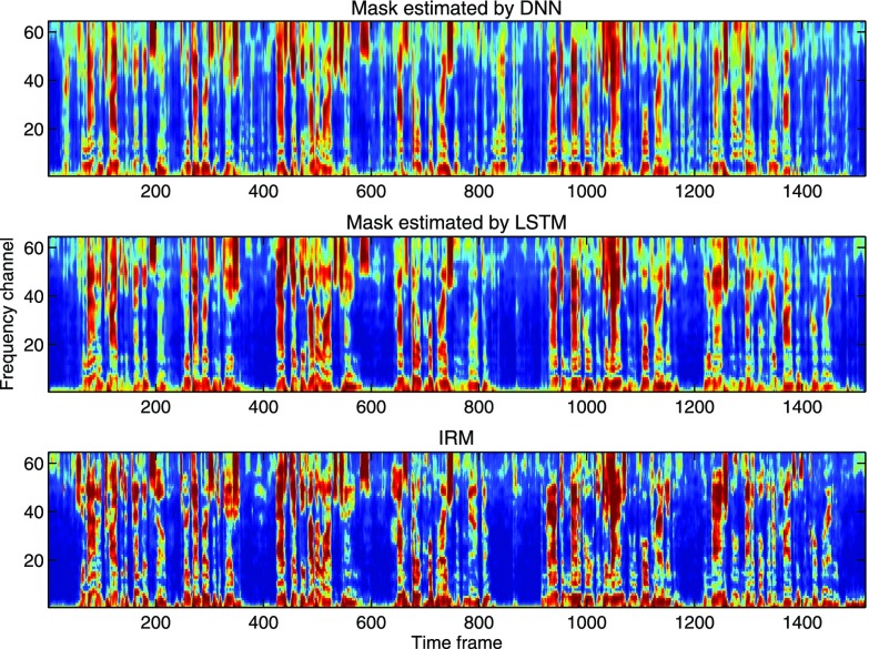
Compared to the speaker-independent DNN, the speaker-independent LSTM substantially improves the performance in terms of the MSE and the STOI improvement. The STOI improvement of LSTM is 7.8% higher than the DNN with the unseen babble noise at −5 dB SNR. This clearly indicates that LSTM achieves better speaker generalization than the DNN. We visualize estimated masks by the DNN and LSTM in Fig. 6, and observe that LSTM reduces the error of mistaking the background noise for target speech (e.g., around frame 850) and better preserves target speech (e.g., around frame 1425).
FIG. 6.
(Color online) Visualization of the estimated masks by the DNN (top), LSTM (middle), and the IRM (bottom). The mixture is created by mixing an unseen male speaker with the unseen babble noise at −5 dB SNR.
C. Model comparisons
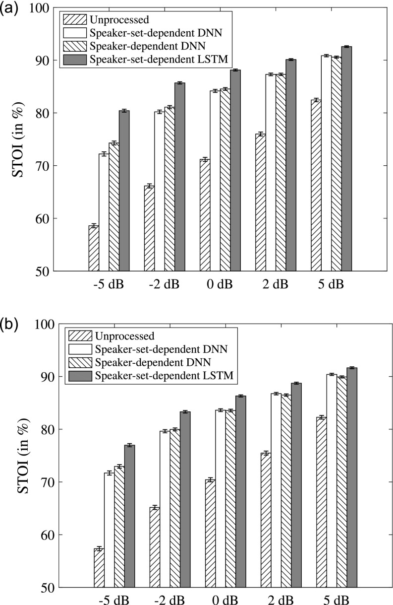
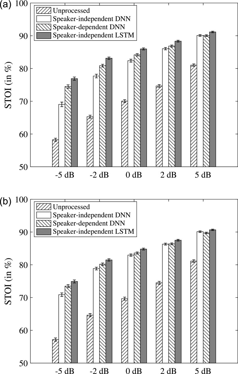
We evaluate speaker-dependent, speaker-set-dependent and speaker-independent models with the babble and cafeteria noise at {−5, −2, 0, 2, 5} dB SNRs. Figure 7 compares speaker-set-dependent DNN, speaker-set-dependent LSTM and speaker-dependent DNN. The speaker-independent DNN, speaker-independent LSTM, and speaker-dependent DNN are compared in Fig. 8. On the one hand, Fig. 7 show that speaker-set-dependent LSTM with 77 training speakers outperforms both speaker-dependent and speaker-set-dependent DNNs, indicating that LSTM learns from other speakers to improve the performance on the six seen speakers. On the other hand, as shown in Fig. 8, speaker-independent LSTM outperforms both speaker-dependent and speaker-independent DNNs on the six unseen speakers, especially at the very low SNR of −5 dB. LSTM also performs well at the unseen SNRs of 2 and 5 dB, demonstrating that LSTM generalizes to unseen noises, unseen speakers and unseen SNRs. We apply paired t-tests with a significance level of 0.01 and find that the improvement of the LSTM over the DNN is statistically significant for both seen and unseen speakers at every test SNR.
FIG. 7.
Comparison of speaker-set-dependent models (trained on 77 speakers and tested on six seen speakers) and speaker-dependent models in terms of STOI. Group means and standard errors are shown. (a) Performance with the unseen babble noise. (b) Performance with the unseen cafeteria noise.
FIG. 8.
Comparison of speaker-independent models (trained on 77 speakers and tested on six unseen speakers) and speaker-dependent models in terms of STOI. Group means and standard errors are shown. (a) Performance with the unseen babble noise. (b) Performance with the unseen cafeteria noise.
In addition to the babble and cafeteria noise, we have tested speaker-independent DNN and LSTM on two other unseen noises, namely, the factory noise and the speech shape noise (SSN). For the factory noise, LSTM improves the processed STOI over DNN by 3.7% and 2.0% at −5 and −2 dB, respectively. For SSN, LSTM improves by 5.0% and 2.0% at −5 and −2 dB, respectively.
D. Analysis of LSTM internal representations
As we discussed in Sec. II, LSTM is supposed to memorize long-term contexts to help mask estimation at a current frame. We analyze what LSTM has learned by visualizing the memory cells ct in Eq. (6) across time frames. Since different memory cells have different dynamic ranges, we map the value range of each memory cell to for better visualization:
| (14) |
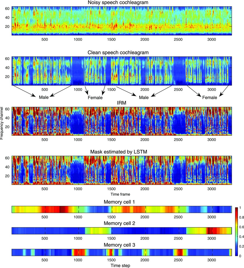
where cmin and cmax denote the minimum and maximum values of a memory cell according to a long-term observation, respectively. Although the internal representations of LSTM are usually distributed and not intuitive, we find a few memory cells that exhibit interesting temporal patterns. We select three memory cells in the third LSTM layer and depict them in Fig. 9. As shown in the bottom three plots of Fig. 9, the first memory cell is excited by male speech and inhibited by female speech. The second cell is activated by female speech. The third one detects a silent interval following target speech after a few frames of delay. These patterns suggest that memory cells encode speech contexts.
FIG. 9.
(Color online) Visualization of speech patterns and memory cell values. Four utterances of two unseen speakers (male and female) are concatenated and mixed with the unseen babble noise at 0 dB SNR. The top four plots depict noisy speech cochleagram, clean speech cochleagram, the IRM and the estimated mask by LSTM, respectively. The bottom three plots show values of three different cells across time, respectively.
Besides memory cells, LSTM also takes previous hidden activations as input. Therefore, the total information from previous time steps is encoded by both and . Since our proposed model has four LSTM layers, the past information can be represented as the concatenation of eight vectors:
| (15) |
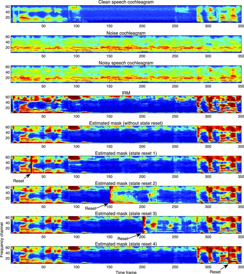
To verify if vstate carries useful information, we reset it to a zero vector to erase past information at different time steps and examine the impact on subsequent mask estimation. We separately reset vstate in speech-dominant and noise-dominant intervals and visualize the resulting estimated masks in Fig. 10. The sixth and ninth plots of Fig. 10 show that resetting vstate during speech-dominant intervals does not make much difference as LSTM appears to quickly recapture the target speaker after observing strong target speech patterns in a few subsequent time steps. However, resetting vstate during noise-dominant intervals may degrade mask estimation for a considerable duration, as shown in the seventh and eighth plots of Fig. 10. LSTM is likely distracted by interfering speech contained in the background and focuses on wrong patterns until strong target-speech patterns are observed. In other words, LSTM seems to be context-aware and keep track of a target speaker for better mask estimation at a current frame.
FIG. 10.
(Color online) Impact of resetting the internal states of LSTM. The top five plots show the clean speech cochleagram, noise cochleagram, noisy speech cochleagram, the IRM, and the estimated mask by LSTM, respectively. The sixth and ninth plots show the estimated masks when LSTM internal states are reset during speech-dominant intervals. The seventh and eighth plots show the estimated masks when LSTM internal states are reset during noise-dominant intervals.
E. Impact of future frames
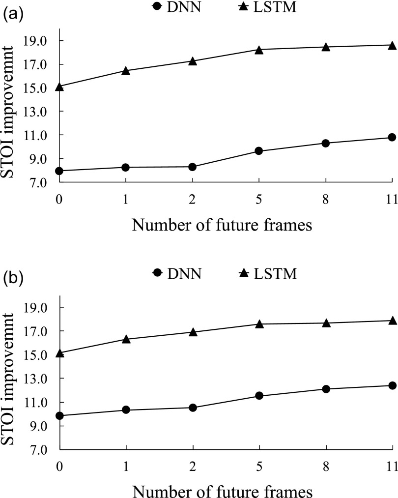
In the above experiments, we use 23 time frames, including 11 future frames, of acoustic features for both the DNN and LSTM. Incorporating future frames improves mask estimation but impedes real-time implementation. To investigate the impact of future frames, we evaluate the models with different asymmetric windows on six unseen speakers and the unseen babble noise at −5 and −2 dB SNRs. Each asymmetric window contains 11 past frames, a current frame and a different number of future frames. We do not decrease the past frames as they facilitate learning and do not violate causality. Figure 11 compares the impact of future frames on the DNN and LSTM. As shown in Figs. 11(a) and 11(b), LSTM substantially outperforms the DNN in all conditions. It is worth noting that LSTM without future frames still outperforms the DNN with 11 future frames, and gives about 15% STOI improvement over unprocessed speech in both SNR conditions.
FIG. 11.
Impact of future frames on the performance of the DNN and LSTM in terms of STOI improvement (in %). The input contains 11 past frames, a current frame and {0, 1, 2, 5, 8, 11} future frames. The models are evaluated with six unseen speakers and the unseen babble noise. (a) Performance of the DNN and LSTM at −5 dB SNR. (b) Performance of the DNN and LSTM at −2 dB SNR.
V. DISCUSSION
In this study, we have investigated speaker generalization of noise-independent models for supervised speech separation. Our previous investigation has demonstrated that a DNN, when trained with a large variety of noises but a fixed speaker, generalizes to unseen noises and unseen SNRs (Wang and Wang, 2013; Chen et al., 2016b). However, real world applications desire a model to perform well with both unseen speakers and unseen noises. Our experimental results show that training of a DNN with many speakers does not perform well on both seen and unseen speakers. This reveals the limited capacity of DNN in modeling a large number of speakers. As a DNN is exposed to more training speakers, the performance on seen speakers drops, suggesting that it fails to focus on a target speaker. A DNN makes independent mask estimation given a window of acoustic features, which appear insufficient to characterize a target speaker for the sake of speech separation.
We have proposed a separation model based on LSTM to improve speaker generalization. The proposed model treats mask estimation as a sequence-to-sequence mapping problem. By modeling temporal dynamics of speech, LSTM utilizes previous inputs to characterize and memorize a target speaker. Therefore mask estimation depends on both the current input and LSTM internal states. By visualizing the temporal patterns of LSTM memory cells, we find that the cell values correlate with speech patterns. Those memory cells capture different contexts to improve mask estimation at a current frame. By resetting LSTM internal states in both speech-dominant and noise-dominant intervals, we find that LSTM appears to detect and focus on a target speaker to help resolve the confusability of speech and noise patterns.
The proposed model substantially outperforms an already strong DNN baseline on both seen and unseen speakers. Interestingly, with more training speakers, the DNN performance on seen speakers degrades, while LSTM improves the results on seen speakers. This reveals the capacity of LSTM in modeling individual speakers. In addition, we have evaluated the dependency of DNN and LSTM on future frames for separation. Our experimental results show that LSTM without future frames still significantly outperforms the DNN with 11 future frames. The proposed model represents a major step towards speaker- and noise-independent speech separation.
ACKNOWLEDGMENTS
This research was supported in part by an AFOSR grant (FA9550-12-1-0130), an NIDCD grant (R01 DC012048), and the Ohio Supercomputer Center.
References
- 1. Bengio, Y. , Simard, P. , and Frasconi, P. (1994). “ Learning long-term dependencies with gradient descent is difficult,” IEEE Trans. Neural Networks 5, 157−166. 10.1109/72.279181 [DOI] [PubMed] [Google Scholar]
- 2. Chen, J. , and Wang, D. L. (2016). “ Long short-term memory for speaker generalization in supervised speech separation,” in Proceedings of INTERSPEECH, pp. 3314−3318. [DOI] [PMC free article] [PubMed] [Google Scholar]
- 3. Chen, J. , Wang, Y. , and Wang, D. L. (2016a). “ Noise perturbation for supervised speech separation,” Speech Commun. 78, 1−10. 10.1016/j.specom.2015.12.006 [DOI] [PMC free article] [PubMed] [Google Scholar]
- 4. Chen, J. , Wang, Y. , Yoho, S. E. , Wang, D. L. , and Healy, E. W. (2016b). “ Large-scale training to increase speech intelligibility for hearing-impaired listeners in novel noises,” J. Acoust. Soc. Am. 139, 2604−2612. 10.1121/1.4948445 [DOI] [PMC free article] [PubMed] [Google Scholar]
- 5. Ephraim, Y. , and Malah, D. (1984). “ Speech enhancement using a minimum-mean square error short-time spectral amplitude estimator,” IEEE Trans. Acoust., Speech, Signal Process. 32, 1109−1121. 10.1109/TASSP.1984.1164453 [DOI] [Google Scholar]
- 6. Erdogan, H. , Hershey, J. R. , Watanabe, S. , and Le Roux, J. (2015). “ Phase-sensitive and recognition-boosted speech separation using deep recurrent neural networks,” in Proceedings of ICASSP, pp. 708−712. [Google Scholar]
- 7. Erkelens, J. S. , Hendriks, R. C. , Heusdens, R. , and Jensen, J. (2007). “ Minimum mean-square error estimation of discrete Fourier coefficients with generalized gamma priors,” IEEE Trans. Audio, Speech, Lang. Process. 15, 1741−1752. 10.1109/TASL.2007.899233 [DOI] [Google Scholar]
- 8. Gers, F. A. , Schmidhuber, J. , and Cummins, F. (2000). “ Learning to forget: Continual prediction with LSTM,” Neural Comput. 12, 2451−2471. 10.1162/089976600300015015 [DOI] [PubMed] [Google Scholar]
- 9. Graves, A. , Mohamed, A. , and Hinton, G. (2013). “ Speech recognition with deep recurrent neural networks,” in Proceedings of ICASSP, pp. 6645−6649. [Google Scholar]
- 10. Healy, E. W. , Yoho, S. E. , Chen, J. , Wang, Y. , and Wang, D. L. (2015). “ An algorithm to increase speech intelligibility for hearing-impaired listeners in novel segments of the same noise type,” J. Acoust. Soc. Am. 138, 1660−1669. 10.1121/1.4929493 [DOI] [PMC free article] [PubMed] [Google Scholar]
- 11. Healy, E. W. , Yoho, S. E. , Wang, Y. , and Wang, D. L. (2013). “ An algorithm to improve speech recognition in noise for hearing-impaired listeners,” J. Acoust. Soc. Am. 134, 3029−3038. 10.1121/1.4820893 [DOI] [PMC free article] [PubMed] [Google Scholar]
- 12. Hochreiter, S. , and Schmidhuber, J. (1997). “ Long short-term memory,” Neural Comput. 9, 1735−1780. 10.1162/neco.1997.9.8.1735 [DOI] [PubMed] [Google Scholar]
- 13. Huang, P.-S. , Kim, M. , Hasegawa-Johnson, M. , and Smaragdis, P. (2015). “ Joint optimization of masks and deep recurrent neural networks for monaural source separation,” IEEE/ACM Trans. Audio, Speech, Lang. Process. 23, 2136−2147. 10.1109/TASLP.2015.2468583 [DOI] [Google Scholar]
- 14. Hummersone, C. , Stokes, T. , and Brookes, T. (2014). “ On the ideal ratio mask as the goal of computational auditory scene analysis,” in Blind Source Separation, edited by Naik G. R. and Wang W. ( Springer, Berlin: ), pp. 349−368. [Google Scholar]
- 15. Jozefowicz, R. , Zaremba, W. , and Sutskever, I. (2015). “ An empirical exploration of recurrent network architectures,” in Proceedings of ICML, 2342−2350. [Google Scholar]
- 16. Kim, G. , Lu, Y. , Hu, Y. , and Loizou, P. C. (2009). “ An algorithm that improves speech intelligibility in noise for normal-hearing listeners,” J. Acoust. Soc. Am. 126, 1486−1494. 10.1121/1.3184603 [DOI] [PMC free article] [PubMed] [Google Scholar]
- 17. Kingma, D. , and Ba, J. (2015). “ Adam: A method for stochastic optimization,” in preprint arXiv:1412.6980, pp. 1−15.
- 18. Kolbæk, M. , Tan, Z.-H. , and Jensen, J. (2017). “ Speech intelligibility potential of general and specialized deep neural network based speech enhancement systems,” IEEE/ACM Trans. Audio, Speech, Lang. Process. 25, 153−167. 10.1109/TASLP.2016.2628641 [DOI] [Google Scholar]
- 19. Loizou, P. C. (2013). Speech Enhancement: Theory and Practice, 2nd ed. ( CRC Press, Boca Raton, FL: ), Chaps. 5−8, pp. 93−376. [Google Scholar]
- 20. Nair, V. , and Hinton, G. E. (2010). “ Rectified linear units improve restricted Boltzmann machines,” in Proceedings of ICML, pp. 807−814. [Google Scholar]
- 21. Ng, J. , Hausknecht, M. , Vijayanarasimhan, S. , Vinyals, O. , Monga, R. , and Toderici, G. (2015). “ Beyond short snippets: Deep networks for video classification,” in Proceedings of CVPR, pp. 4694−4702. [Google Scholar]
- 22. Pascanu, R. , Mikolov, T. , and Bengio, Y. (2013). “ On the difficulty of training recurrent neural networks,” in Proceedings of ICML, pp. 1310−1318. [Google Scholar]
- 23. Paul, D. B. , and Baker, J. M. (1992). “ The design for the Wall Street Journal-based CSR corpus,” in Proceedings of the Workshop on Speech and Natural Language, pp. 357−362. [Google Scholar]
- 24. Sak, H. , Senior, A. W. , and Beaufays, F. (2014). “ Long short-term memory recurrent neural network architectures for large scale acoustic modeling,” in Proceedings of INTERSPEECH, pp. 338−342. [Google Scholar]
- 25. Srinivasan, S. , Roman, N. , and Wang, D. (2006). “ Binary and ratio time-frequency masks for robust speech recognition,” Speech Commun. 48, 1486–1501. 10.1016/j.specom.2006.09.003 [DOI] [Google Scholar]
- 26. Sun, D. , and Mysore, G. (2013). “ Universal speech models for speaker independent single channel source separation,” in Proceedings of ICASSP, pp. 141−145. [Google Scholar]
- 27. Sundermeyer, M. , Ney, H. , and Schlüter, R. (2015). “ From feedforward to recurrent LSTM neural networks for language modeling,” IEEE/ACM Trans. Audio, Speech, Lang. Process. 23, 517−529. 10.1109/TASLP.2015.2400218 [DOI] [Google Scholar]
- 28. Sutskever, I. , Vinyals, O. , and Le, Q. V. (2014). “ Sequence to sequence learning with neural networks,” in Proceedings of NIPS, 3104−3112. [Google Scholar]
- 29. Taal, C. H. , Hendriks, R. C. , Heusdens, R. , and Jensen, J. (2011). “ An algorithm for intelligibility prediction of time-frequency weighted noisy speech,” IEEE Trans. Audio, Speech, Lang. Process. 19, 2125−2136. 10.1109/TASL.2011.2114881 [DOI] [Google Scholar]
- 30. Wang, D. L. (2005). “ On ideal binary mask as the computational goal of auditory scene analysis,” in Speech separation by humans and machines, edited by Divenyi P. ( Kluwer, Boston, MA: ), pp. 181−197. [Google Scholar]
- 31. Wang, D. L. , and Brown, G. J. , Eds. (2006). Computational Auditory Scene Analysis: Principles, Algorithms and Applications ( Wiley-IEEE, Hoboken, NJ: ), Chap. 1, pp. 1−44. [Google Scholar]
- 32. Wang, Y. , Narayanan, A. , and Wang, D. L. (2014). “ On training targets for supervised speech separation,” IEEE/ACM Trans. Audio, Speech, Lang. Process. 22, 1849−1858. 10.1109/TASLP.2014.2352935 [DOI] [PMC free article] [PubMed] [Google Scholar]
- 33. Wang, Y. , and Wang, D. L. (2013). “ Towards scaling up classification-based speech separation,” IEEE Trans. Audio, Speech, Lang. Process. 21, 1381−1390. 10.1109/TASL.2013.2250961 [DOI] [Google Scholar]
- 34. Weninger, F. , Erdogan, H. , Watanabe, S. , Vincent, E. , Le Roux, J. , Hershey, J. R. , and Schuller, B. (2015). “ Speech enhancement with LSTM recurrent neural networks and its application to noise-robust ASR,” in Proceedings of LVA/ICA, pp. 91−99. [Google Scholar]
- 35. Williams, R. J. , and Peng, J. (1990). “ An efficient gradient-based algorithm for on-line training of recurrent network trajectories,” Neural Comput. 2, 490−501. 10.1162/neco.1990.2.4.490 [DOI] [Google Scholar]
- 36. Xu, Y. , Du, J. , Dai, L.-R. , and Lee, C.-H. (2014). “ An experimental study on speech enhancement based on deep neural networks,” IEEE Signal Process. Lett. 21, 65−68. 10.1109/LSP.2013.2291240 [DOI] [Google Scholar]
- 37. Zhao, X. , Wang, Y. , and Wang, D. (2014). “ Robust speaker identification in noisy and reverberant conditions,” IEEE/ACM Trans. Audio, Speech, Lang. Process. 22, 836−845. 10.1109/TASLP.2014.2308398 [DOI] [Google Scholar]


