Impacting the effect of fMRI noise through hardware and acquisition choices – implications for controlling false positive rates

Abstract

We review the components of time-series noise in fMRI experiments and the effect of image acquisition parameters on the noise. In addition to helping determine the total amount of signal and noise (and thus temporal SNR), the acquisition parameters have been shown to be critical in determining the ratio of thermal to physiological induced noise components in the time series. Although limited attention has been given to this latter metric, we show that it determines the degree of spatial correlations seen in the time-series noise. The spatially correlations of the physiological noise component are well known, but recent studies have shown that it can lead to a higher than expected false-positive rate in cluster-wise inference based on parametric statistical methods used by many researchers. Based on understanding the effect of acquisition parameters on the noise mixture, we propose several acquisition strategies that might be helpful reducing this elevated false-positive rate, such as moving to high spatial resolution or using highly-accelerated acquisitions where thermal sources dominate. We suggest that the spatial noise correlations at the root of the inflated false-positive rate problem can be limited with these strategies, and the well-behaved spatial autocorrelation functions (ACFs) assumed by the conventional statistical methods are retained if the high resolution data is smoothed to conventional resolutions.

Introduction

Applied to the intensity fluctuations of a pixel in an fMRI time-series, the term “noise” is so non-specific and carries such negative connotations that it should probably be eliminated from the fMRI vocabulary. Many components of the fluctuations derive from physiological processes that may well be of interest, such as the temporally correlated components used in resting-state fMRI. Nonetheless, there are nuisance components to the temporal fluctuations, some of which fit the term “noise” well since they derive from conventional random processes (such as electrical losses in the tissue as well as in the RF detector and preamplifier). These fluctuations are typically referred to as “thermal” following the analysis of fluctuations in electronic systems using statistical physics through the fluctuation-dissipation theorem, which focuses extensively on their temperature dependence (not of direct interest to fMRI). The thermal fluctuations are statistically independent between measurements and thus spatially and temporally uncorrelated in the image time-series. They are characterized by a Gaussian distribution of the signal amplitude. Kellman et al. described how to characterize the thermal noise in a single image so that this single-image noise level also describes the fluctuations expected in a pixel time-series series derived from perfectly repeating that image acquisition. (Kellman and McVeigh, 2005) In phantom images from a well-tuned scanner, the time-series fluctuations are completely dominated by these thermal components, and noise observed from a single image completely describes the observed time-series variance.

The thermal noise component, however, far from fully accounts for the fluctuations in a typical fMRI time series. For example, the non-thermal component is 3 to 4 fold higher for a 3 mm isotropic voxel EPI time-series at 3T using a modern array coil. (Triantafyllou et al., 2011) Since they are only present in living samples, we loosely refer to these other noise sources as “physiological noise.” Physiological noise sources arise since sensitivity to metabolic changes is mission-critical for the fMRI acquisition. Thus we expect the fMRI time-series to be further modulated by, at the very least, fluctuations in blood flow and metabolism associated with “resting-state” or spontaneous neuronal firing, which is seen in electrophysiology and EEG to fluctuate in a complex way that appears noise-like.[Yuan et al. 2012, Britz et al. 2010] Thus neuronal activity unrelated to the task of interest might be labeled “noise.” Multiple other sources also modulate the image intensity in the time-series in complex “noise-like” ways. These include: hemodynamic fluctuations associated with the cardiac and respiratory cycle [Glover et al 2000, Hu et al 1995, Dagli et al 1999] as well as slow changes in the heart rate [Chang et al. 2009] and respiratory volume [Birn et al. 2008], B₀ shifts associated with these cycles [Van de Moortele et al 2002, Raj et al 2001], rigid and non-rigid tissue motion [Soellinger et al. 2009, Poncelet et al 1992], low-frequency changes such as vasomotion [Mayhew et al 1996, Wise et al 2004], and CSF flow [Klose et al. 2000, Greitz et al 1987]. The origins of many of these noise fluctuations are surveyed in detail elsewhere in this Special Issue. To the extent that we cannot fully predict these fluctuations, we call them “physiological noise”, although the term “signal clutter” is a better descriptor. Because of their complex but not truly random origin, these sources of time-series variance are not as easy to statistically account for. The important distinction we will use when modeling these fluctuations is that they are modulations of the signal (i.e., multiplicative noise), and thus proportional to the signal level, whereas thermal noise is superimposed on top of any signal changes and its amplitude is independent of the signal level (i.e., additive noise). For example, if the imaging flip angle is set to 0°, the signal—and thus all physiological noise in the time-series—disappears but the thermal noise fluctuations are left.

The importance of noise in statistical analysis of fMRI data

In short, any signal that lands in the residual to a model fit in a task-based study is termed “noise” and, as such, is the basis for determining the statistical significance of the reported activation. Given this significance, the time-series variance has always been an important part of characterizing the fMRI measurement. But recently, the importance of understanding the fMRI noise types, especially the relative contributions of thermal and non-thermal sources, has been underscored by a study of false-positive rates in task-based fMRI data.(Eklund et al., 2016) This study made use of large databases of existing resting-state data (Biswal et al., 2010; Yan et al., 2013) to assess the generation of false positive activation when the task-free data was analyzed for various task-evoked activations. In this scheme, any observed activation is identified as a false-positive. The result was a surprisingly high false-positive rate for common processing pipelines like FSL, AFNI, and SPM when making cluster-wise inferences about activation using relatively large clusters (low Cluster Defining Thresholds). We refer to the general issue raised by Eklund et al. for parametric analysis using cluster-wise inferences as the “False-Positive Rate (FPR) problem”.

The culprit likely arises from the simplifying assumptions made in the statistical calculations regarding the noise correlations between neighboring voxels. In a noise model which assumes that the time-series noise is thermal (Gaussian distributed and spatially uncorrelated), activation in neighboring voxels is a strong indication of non-spurious activation. But, if the noise is, in fact, more spatially correlated than assumed, observing activation in neighboring voxels is less indicative of statistical significance. Clustering of activation will be seen even for spuriously activated pixels and the analysis will over-claim the significance of the clustered activation (false positive).

Thus, assuming thermal noise characteristics for a time-series dominated by non-thermal, spatially correlated fluctuations places practitioners in danger of labeling spurious fluctuations as neuronal activation if they overly rely on cluster-wise tests to discount false positive activation. While we have known for decades that the noise model assumed by common analysis packages is not fully correct, the Eklund et al. study has highlighted the danger of ignoring the non-thermal nature of the fluctuations in standard acquisitions analyzed with standard parametric cluster-wise inferences.

Potential for mitigating the false positive problem via the acquisition

Fortunately, while we know the time-series variance is not entirely thermal, we can characterize the fraction of thermal to non-thermal noise. We also know quite a bit about how this ratio varies with hardware and acquisition choices. In fact, the user can effectively set this ratio to whatever value is deemed adequate to render the time-series fluctuations essentially Gaussian and un-correlated spatially. In this case, the assumptions of the standard statistical tests are valid. Furthermore the user can experimentally verify that the desired noise mixture has been achieved. This empowers us to alter future acquisition protocols to try to minimize the false-positive problem through acquisition choices. This approach is also compatible with other responses to the false-positive problem which have supported preserving the existing statistical parametric mapping framework but paying careful attention to the analysis. (Flandin and Friston, 2016; Mumford et al., 2016)

Sadly, the evolution of improved imaging hardware (higher field strength and better array coils) has likely exacerbated the false-positive problem by increasing the signal to thermal noise ratio (SNR₀) in the images. The hardware improvements also increase signal levels which we will see as increases the physiological noise component. Thus, while these improvements aid fMRI sensitivity, they increase ratio of physiological to thermal noise in the image time-series. The hardware improvements have made modern fMRI acquisitions more physiological noise dominated than older, lower field and/or single-channel acquisitions. This suggests that many older studies are likely less non-thermally dominated than the modern acquisitions analyzed by Eklund et al. It is possible that they are therefore not as prone to the inflated false-positive rate problem as the data used the Eklund et al. study. Nonetheless, the effect of improved detection sensitivity on the noise mixture should be carefully considered for future studies. Luckily, there are potential acquisition strategies that can likely improve the FPR problem without reverting back to lower sensitivity detection.

Given the physiological noise source of the FPR problem and its overall importance to the fMRI field, this review concentrates on how hardware and acquisition choices affect the ratio of thermal to non-thermal noise in the fMRI time-series and thus the false-positive problem. We concentrate on identifying strategies that tip this ratio back toward thermal noise dominance—but in a smarter way then simply desensitizing the acquisition or adding noise. The goal is to render the assumptions about the time-series variance (specifically spatial correlations) used in common statistical analysis packages more accurate in their description of the noise, yielding acceptable false-positive rates.

The physiological to thermal noise ratio

The Krueger-Glover model (Kruger and Glover, 2001) describes the relationship between the signal-to-noise ratio in an individual image (SNR₀), and the time-series SNR (tSNR). Both SNR measures are defined on a pixel-wise basis, but of course, can also be analyzed in ROIs. The SNR₀ is defined by the pixel’s signal level, S, and the thermal image noise standard deviation, σ₀. The image noise SD, σ₀, is typically gleaned from the k-space data acquired in the absence of a transmit pulse (zero degree flip angle excitation), which is devoid of all signal. Care must be taken in array coil acquisitions to properly account for how the image reconstruction and array channel combination processes scale the noise measured in k-space into the image noise SD, σ₀. (Kellman and McVeigh, 2005; Roemer et al., 1990)

The tSNR of a pixel is the ratio of S and the total standard deviation in the time-series fluctuations, σ_t, simply measured by calculating the variance of that pixel’s intensity over the time-series. In the Krueger-Glover model, ${\sigma }_t^2$ is analyzed as a combination of ${\sigma }_0^2$ and the physiological noise variance, ${\sigma }_P^2$; i.e., ${\sigma }_t^2={\sigma }_0^2+{\sigma }_P^2$. The thermal image noise variance ${\sigma }_0^2$ is independent of the MR signal level since it mainly derives from electrical losses in the body, coil components and preamplifier. In contrast, Krueger and Glover showed that ${\sigma }_P^2$ is proportional to the MR signal level (S) in the voxel with a proportionality constant λ; σ_P = λS. As the signal level increases, the physiological noise increases and eventually becomes dominant. Thus, increasing signal levels and decreasing image noise (for example by operating at higher field strength, higher flip angle, or improving detection coils) does not necessarily directly pay off in greatly improved tSNR. The tSNR reaches an asymptotic limit (shown to be 1/λ) that is independent of the SNR₀. Simple manipulations of these definitions leads to the relationship between tSNR and SNR₀:

$$\mathit{tSNR}=\frac{SN{R}_0}{\sqrt{1+{\lambda }^2·SN{R}_0^2}}.$$ [1]

The above analysis has also been shown to hold when the SNR₀ is modulated by field strength and/or voxel volume (Triantafyllou et al., 2005) as well as the original demonstration of based on varying the flip-angle (Kruger and Glover, 2001). It has been extended to include the correlation between channels in an array coil (Hutton et al., 2012; Triantafyllou et al., 2011) as well as noise correlations in the array that do not obey a simple scaling with signal intensity (Triantafyllou et al., 2016). Bodurka et al. showed different tissues have different asymptotes (1/λ) with white matter having the highest potential tSNR and CSF the lowest. (Bodurka et al., 2007) Note that through the relationship ${\sigma }_t^2={\sigma }_0^2+{\sigma }_P^2$, this model itself assumes that the physiological fluctuations are Gaussian and temporally uncorrelated. Nonetheless, the model has proved useful.

Calculating the physiological to thermal noise ratio, σ_P/σ₀, is also straightforward, and can be determined from a single measurement of both SNR₀ and tSNR:

$$\frac{{\sigma }_P}{{\sigma }_0}=\sqrt{{\left(\frac{SN{R}_0}{\mathit{tSNR}}\right)}^2-1}.$$ [2]

Note that if this formula is used, the thermal (single-image) SNR₀ needs to be calculated using all the factors introduced by Kellmann et al. in order for it to be directly comparable to the tSNR measure.(Kellman and McVeigh, 2005) For example, simply computing SNR₀ using an ROI in the image as a measure of S and an ROI in the noise region outside the head as a measure of σ₀ is not sufficient when considering images acquired with array coils.

Triantafyllou et al. showed how the measured physiological-to-thermal noise ratio increases with field strength (1.5T, 3T and 7T) and changed with spatial resolution for a single-channel birdcage coil.(Triantafyllou et al., 2005) These results are reproduced here in Fig. 1. Note that this work used older single-channel coils. The physiological-to-thermal noise ratios increase when array coils are used (since S increases). Table 1, reproduced from Triantafyllou et al. (Triantafyllou et al., 2011), lists measured physiological-to-thermal noise ratios for a 3T time-series acquired at differing spatial resolution and modern array coil designs.

Fig. 1. Physiological-to-thermal-noise ratio as a function of acquisition voxel volume (reproduced from Triantafyllou et al.).

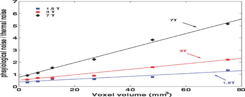
The ratio σ_p/σ₀ is observed to decrease approximately linearly with voxel volume. Data are from single-channel coil measurements at 1.5T, 3T and 7T.

Table 1.

Ratio of σ_p/σ₀ calculated from the SNR₀ and tSNR measurements for each coil and spatial resolution for 3T acquisitions.

Resolution (mm3)	Single Ch	12Ch rSoS	12Ch ncov-w-rSoS	32Ch rSoS	32Ch ncov-w-rSoS
1×1×3	0.28±0.21	0.52±0.05	0.79±0.10	1.34±0.12	1.80±0.15
1.5×1.5×3	0.42±0.35	0.86±0.07	1.25±0.11	2.04±0.17	2.73±0.18
2×2×3	0.46±0.33	0.90±0.10	1.62±0.12	2.87±0.14	3.96±0.13
3×3×3	0.51±0.10	1.20±0.08	1.99±0.18	3.03±0.13	4.13±0.15
4×4×3	0.65±0.15	1.91±0.13	2.79±0.21	3.93±0.29	5.28±0.40
5×5×3	0.89±0.16	2.26±0.15	3.27±0.26	5.28±0.28	7.08±0.38

In addition to calculating σ_p/σ₀ using Eq. 2, the mixture of physiological to thermal noise can be assessed qualitatively by simply looking at a tSNR map. If the time-series is thermal noise (image noise) dominated, the tSNR map will look similar to an SNR₀ map. In these maps the tSNR simply follows the receive array’s sensitivity profile, falling monotonically from the exterior of the head to a minimum in the center of the head. In contrast, if the time-series is physiological noise dominated, the tSNR map tends to be more spatially uniform across the head and reflects anatomical features. Generally white matter is the “quietest” and so tSNR is highest within the white matter. Gray matter has higher physiological noise variance and CSF even more. (Bodurka et al., 2007; Triantafyllou et al., 2016) For the thermal noise dominated case, the SNR₀ and the tSNR maps tend to have the same overall pattern (that of the coil sensitivity profile). This is seen in the 1×1×3mm³ acquisition in Fig. 2. In contrast, the two types of SNR map look very different in the 3×3×3mm³ acquisition that is physiological noise dominated. Here the tSNR reflects the anatomy (WM having high tSNR and GM and CSF lower) rather than the coil sensitivity profile.

Fig. 2. Spatial distribution of tSNR for thermal-noise- and physiological-noise dominated acquisitions.

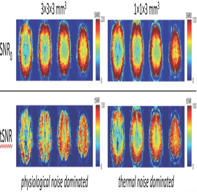
SNR₀ (top row) and tSNR (bottom row) for 3T acquisitions with decreasing voxel size. (different color scales were used to highlight spatial distribution of SNR.) As voxel size decreases, the dominant source noise shifts from physiological (in the 3×3×3 mm³ data) to thermal (in the 1×1×3 mm³ data). The spatial distribution of tSNR for a physiological-noise dominated acquisition resembles the anatomy—low-noise tissues like white matter exhibit high tSNR, while noisy regions such as those containing CSF exhibit low tSNR. The spatial distribution of tSNR for a thermal-noise-dominated acquisition more closely resembles SNR₀, and tSNR is largely a function of the distance from the surface receive coils arranged around the head—in axial images acquired with a helmet surface-coil array SNR₀ is high around the edges of the brain and falls off smoothly towards the center of the brain.

The use of parallel imaging acceleration of an acquisition can also effect the σ_p/σ₀ ratio. Figure 3 shows the tSNR profiles transitioning from the physiological noise dominance pattern (seen for the R=1 acquisition) into the thermal noise dominating pattern (seen in the R=3 and R=4 acquisition). In this case, the parallel imaging acceleration is amplifying the thermal noise through both the √R noise penalty and the g-factor noise enhancement, with little effect on physiological noise. (de Zwart et al., 2006) Therefore at sufficiently high accelerations, the acquisition becomes thermal noise dominated.

Fig. 3. Effects of parallel imaging acceleration on the balance between thermal and physiological noise.

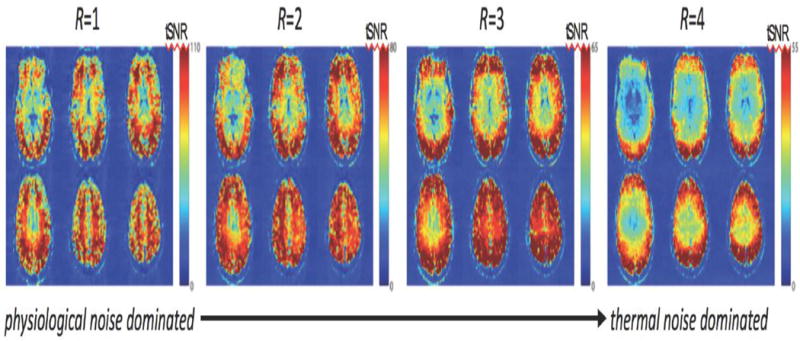
Example tSNR maps acquired from 3T fMRI data. With higher acceleration factors (R) the √R and g-factor noise penalty causes the acquisition to be thermal-noise dominated, and so the spatial pattern of tSNR is mainly a function of the distance from the surface coils.

Effect of the σ_p/σ₀ ratio on the “heavy tail” in the spatial ACF

The Eklund et al. study identified the deviation of the spatial AutoCorrelation Function (ACF) from the squared exponential (Gaussian) pattern expected for thermal noise as the culprit behind the inflated FPRs for cluster-wise inferences. Specifically, the spatial ACFs of in vivo fMRI time-series data show “heavy tails” indicating that the time-series fluctuations have some spatial correlation over multiple pixels. For true thermal noise, the spatial ACF is Gaussian, with a width of one pixel. In this case, the correlation between time-series for pixels more than a few pixel-widths apart is negligible.

To demonstrate how increasing σ_p/σ₀ above unity introduces tails in the spatial ACF of the noise residual, and how they are affected by acquisition and post-processing strategies, we simulated a time-series of 1D noise images. We generated a synthetic 1D spatial map of the time-series noise residual containing a thermal noise component and a physiological noise component. The synthetic thermal noise component is drawn from a Gaussian white-noise distribution uncorrelated in space and time. Therefore its spatial ACF is a Gaussian with a one-pixel FWHM. In other words, the correlation of this 1D noise image with a duplicate version of itself shifted by one or more pixel lengths is nearly zero.

The time-series of 1D images representing the physiological fluctuations do not behave this way. Their ACF is not captured by a Gaussian function and is characterized by a “heavy tail” indicating a very gradual decrease in spatial correlations with distance. In this simulation the physiological noise component was synthesized to have equal amounts of spatial autocorrelations at all spatial scales out to 40 mm FWHM. (This spatial correlation was imposed by convolving synthetic uncorrelated noise with a series of boxcar kernels ranging from 1 to 40 mm in width.) To simulate the total noise seen in a typical acquisition, the synthetic thermal and physiological noise were combined with weighting coefficients taken from the σ_p/σ₀ ratios seen in common fMRI acquisitions. We then applied spatial smoothing to this synthesized total noise to assess its effect on the spatial autocorrelation.

Figure 4 shows the spatial ACFs for two example σ_p/σ₀ ratios. The simulated data were generated assuming a 3 mm native spatial resolution. Note that when σ_p/σ₀ = 0 (representing an acquisition with no physiological noise, Fig. 4a), the spatial ACF is a Gaussian function (by design), but for σ_p/σ₀ = 3.0 (Fig. 4b) the heavy tails of the spatial ACF are evident and the best-fit Gaussian function is a poor representation of the actual ACF. Figure 4c and 4d show the same simulated data smoothed to a 6 mm spatial resolution. For the pure thermal noise case (Fig. 4c), the Gaussian is still a good fit (since a signal with a Gaussian autocorrelation function convolved with another Gaussian kernel will also have a Gaussian autocorrelation function). But the ACF for the σ_p/σ₀ = 3.0 case (Fig. 4d) remains a poor fit to a Gaussian function even after smoothing. The non-Gaussian ACF persists because the modest smoothing does little to average out the correlations which exist on a length-scale longer than the smoothing kernel width.

Fig. 4. The effect of the noise contributions on the spatial ACF in modeled 1D resting-state data.

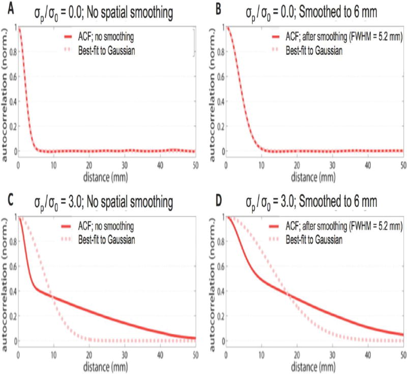
All simulations use a native acquisition resolution of 3 mm. (A) Pure thermal noise, no spatial smoothing. ACF is well characterized by a Gaussian function, as expected for thermal noise. (B) Pure thermal noise, after smoothing to 6 mm FWHM spatial resolution. Spatial ACF is still well described by Gaussian function. (C) Physiological noise dominated case (σ_p/σ₀ = 3.0), no spatial smoothing. The physiological noise component introduces long-range correlations in the noise which produce “heavy tails” in the ACF. (D) Physiological noise dominated case (σ_p/σ₀ = 3.0) after smoothing to 6 mm FWHM spatial resolution. ACF retains non-Gaussian character. Thus the smoothing kernel is not sufficiently broad to impose a Gaussian shape on the ACF.

Strategies to reduce the physiological to thermal noise ratio

These spatial ACF characterizations suggest two options for reducing the physiological-to-thermal noise ratio and thus insuring the validity of the assumptions of the standard cluster-wise inference methods. First, we could consider “dumbing down” the acquisition by using lower fields and/or simpler RF detectors, or perhaps simply adding uncorrelated Gaussian noise. It is not clear that this would be better than simply raising the thresholds for claiming significance. The second, much more attractive option is to acquire the fMRI data with thermal noise dominance such that σ_p/σ₀ < 1. This could be achieved, for example, by using highly accelerated, high spatial resolution acquisitions. Even at 7T, where physiological noise levels are increased substantially compared at 3T, fMRI data measured using 32-channel array coils are thermal-noise dominated when acquired with a modest resolution of 1×1×1 mm³, especially when using the parallel imaging acceleration typically needed to achieve this resolution for BOLD-weighted fMRI.

Most of the σ_p/σ₀ ratio reduction in high spatial resolution acquisition derives from the reduced signal strength. According to the extremely well validated Krueger-Glover model, when the spatial resolution is increased, the signal, and thus the physiological noise contribution, is decreased by a factor of the voxel volume since σ_P = λS. Therefore reducing the acquisition from 3 mm isotropic to 1 mm isotropic reduces both σ_p greatly (27 fold) along with S. In short, in the heavily physiological noise dominated case, both the signal and the noise are reduced by a factor of the voxel volume, resulting in no net loss of tSNR. To the extent that the time-series noise is a mixture of thermal and physiological noise, reducing voxel volume will result in a loss of tSNR, but the tSNR loss is far less than the signal loss. For example, at 3T, reducing the voxel volume 9-fold (from 3×3×3 mm³ to 1×1×3mm³) resulted in only a factor of 1.5 reduction in tSNR.(Triantafyllou et al., 2011)

In contrast, the SNR₀ is drastically reduced since signal scales as the voxel volume and the thermal noise is roughly the same. The thermal image noise is set by the RF detector sensitivity, the imaging sampling bandwidth (BW) (related to the frequency across the FOV) and the parallel imaging acceleration rate and is only secondarily affected by voxel volume. In practice the imaging BW decreases for high-resolution EPI, thus reducing thermal noise in the image data, but the parallel imaging acceleration rate tends to be higher, resulting in little net change in SNR₀ with voxel volume. For example, in going from 3 mm isotropic to 1 mm isotropic resolution the EPI bandwidth decreased 2.2 fold. (Triantafyllou et al., 2011) This alone would reduce σ₀ by √2.22 = 1.48 fold. But, if twice the parallel imaging acceleration was used (which helps achieve the needed image encoding), the decrease in σ₀ would still only be 1.48/√2 = 1.05. Note that the g-factor penalty of higher acceleration factors also pushes the acquisition toward thermal noise dominance since it amplifies only the thermal noise, as seen in Fig. 3 and shown by others (de Zwart et al., 2006).

In addition to in-plane acceleration, adding parallel imaging techniques such as Simultaneous MultiSlice (SMS) also produce g-factor amplification which lowers σ_p/σ₀. Additionally, shorter TR times in SMS acquisitions can necessitate a reduced flip angle to avoid saturation. Krueger and Glover demonstrate that flip-angle reduction directly moves the acquisition toward the thermal noise dominated state. (Kruger and Glover, 2001) Shorter TR times do however lead to greater potential for steady-state coherence pathways between measurements that could be disturbed by B₀ changes driven by the cardiac and respiration cycles (Zhao et al 2000), and therefore could also re-introduce spatial correlations in acquisitions that are not properly spoiled through this mechanism.

However, many fMRI practitioners fear the drastic drop in SNR₀ associated with high resolution imaging (e.g. the 27-fold decrease in SNR₀ expected when dropping from 3 mm to 1 mm isotropic) even though they should be focusing only on tSNR. Once the magnetic field (B₀) and the TE value is chosen, the tSNR is the only acquisition metric which directly reflects the CNR of the BOLD experiment for an activated voxel. In this case, ${\text{CNR}}_{\text{BOLD}}=(\mathrm{\Delta }{\mathrm{R}}_2^{\ast }/{\mathrm{R}}_2^{\ast })·\text{tSNR}$, where ${\mathrm{R}}_2^{\ast }=1/{\mathrm{T}}_2^{\ast }$. Here we assume an optimized TE set to $\text{TE}={\mathrm{T}}_2^{\ast }$. Importantly, the only other factor in the CNR equation, the fractional change in relaxivity relaxation rate on activation $(\mathrm{\Delta }{\mathrm{R}}_2^{\ast }/{\mathrm{R}}_2^{\ast })$, is determined by the biology of the metabolic and blood oxygenation response (and B₀ field strength) but is not directly dependent on the voxel volume or other pulse-sequence acquisition parameters. Thus for a given B₀ and TE, the primary acquisition metric of activation detection sensitivity should be tSNR. As we saw above, the reduction in tSNR, and thus CNR_BOLD, when moving to high spatial resolution acquisitions can be modest.

In many cases, CNR_BOLD might actually improve as spatial resolution is increased. This might happen through reducing partial volume dilution of the activation changes by non-activated white matter or CSF. It is important to keep in mind that the standard practice of acquiring at 3 mm spatial resolution does not spatially resolve the cortex, since the Nyquist criteria requires 2 voxels across the cortex to fully sample the cortex (which for adult human cerebral cortex translates into requiring voxels no larger than about 1.0 mm). Therefore the partial volume issue is significant for standard 3 mm acquisitions and becomes even worse if simple volumetric or 3D spatial smoothing is applied to the fMRI data. Finally, high spatial resolution is, of course, mandatory if the experiment attempts to resolve small functional structures.

Nonetheless, there are some down-sides to increased spatial resolution including potential increases in geometrical distortion in EPI and reduced temporal resolution due to the long readout periods. Increased spatial resolution requires increasing the amount of image encoding, i.e., increasing the number of points in the readout direction and k-space lines acquired in the PE direction. This increases the amount of time spent encoding each imaging slice which increases minimum TE. The longer readouts also reduce the velocity through kspace, increasing distortion from B₀ susceptibility shifts. But multi-channel array coils come into play here, this time helping to mitigate these problems by providing parallel image acceleration capabilities (Griswold et al., 2002; Pruessmann et al., 1999) and Simultaneous MultiSlice (SMS) (Larkman et al., 2001; Moeller et al., 2010) with blipped-CAIPI (Setsompop et al., 2012) EPI. It is important to note, however, that accelerating in the phase-encoding direction (in conventional parallel imaging) places limits on the amount of acceleration achievable for accelerating in the slice-encoding direction (in blipped-CAIPI Simultaneous Multi-Slice parallel imaging),[Setsompop et al 2016] therefore achieving both high conventional acceleration and high slice acceleration requires dense coil arrays.

Achieving thermal noise dominance when high spatial resolution is not of interest

When acquiring at high spatial resolution is not possible or not required for a given study, one strategy for reducing the σ_p/σ₀ ratio of a physiological noise dominated acquisition is to simply reduce the excitation flip angle to reduce the signal and thereby reduce physiological noise fluctuations. If not pushed to far, this strategy has been shown to minimally impact tSNR.(Kruger & Glover 2001, Gonzalez-Castillo et al. 2011) Note however, that the σ_p/σ₀ can not be reduced from σ_p/σ₀ > 1 to σ_p/σ₀ < 1 without adversely effecting the tSNR. Gonzalez-Castillo et al, showed that a reduced flip angle can have benefits of its own such as reduced RF power, limitation of T₁ weighting and thus inflow effects, and reduction of through-plane motion effects. The altered inflow impacts the balance of the multiple hemodynamic components of the fMRI signal, which could also influence the temporal characteristics of the BOLD response, as previously noted.[Gonzalez-Castillo et al. 2011, Renval et al 2014] In some cases, however, this reduction of inflow could be beneficial, nevertheless it is an alteration of the signal as well as the noise.

Another strategy toward decreasing the σ_p/σ₀ ratio is, of course, to regress as much physiological noise out of the data as possible. This is perhaps best achieved by additional, external recordings of systemic physiology, such as the respiratory and cardiac cycles. We rely on other contributions to this special issue to fully review the many methods developed toward removing physiological noise in post-processing. Successful removal would also reduce the spatial correlations which give rise to the tails in the spatial ACF and therefore reduce the false positive rate problem. It can be challenging, however, to relate these external measures to the BOLD signal as they can have complex spatiotemporal effects on the fMRI signals, and it may not be possible fully account for all physiological noise fluctuations.

Fortunately, thermal noise is not only more straightforward to account for in the statistical analysis due to its lack of spatial or temporal correlation, but it is also simpler to remove from the data. Previous studies have noted that applying spatial smoothing to the image time-series asymmetrically effects the physiological and thermal noise contributions. (Triantafyllou et al., 2006) Triantafyllou et al. suggested a method for sidestepping the physiological noise. For example, if a final spatial resolution of 5 mm is desired (a typical final spatial for fMRI statistical analysis packages that spatially smooth the acquired data), this can be achieved in multiple ways. One strategy would be to acquire at 5 mm spatial resolution and not apply spatial smoothing. A second approach would be to acquire at 1.5 mm image resolution and spatially smooth the images to 5 mm resolution in post-processing. The difference is that the high resolution acquisition effectively side-steps physiological noise. Increasing the voxel volume via smoothing during post-processing produces a σ_p growth that is less than linear in voxel-volume, leading to an net improvement in tSNR even for heavily physiological noise dominated acquisitions. In contrast, increasing voxel size at acquisition does not substantially improve tSNR (which remains at its asymptotic limit) in the physiological noise dominated acquisition. Triantafyllou et al. showed that the second strategy (acquiring at 1.5 mm resolution and smoothing to 5 mm) results in a 1.89 fold higher tSNR than the first strategy for a 7T acquisition with a conventional single-channel coil. (Triantafyllou et al., 2006) The tSNR gains afforded by this strategy should be even higher for array coils since the higher sensitivity produces increased physiological noise dominance and even further bounds the tSNR at its asymptotic limit.

In addition to this tSNR benefit, we propose that this strategy (acquire at high spatial resolution then smooth to the desired resolution) also helps to control the heavy tails in the spatial ACFs and thus helps mitigate the false positive rate problem. Designing acquisitions that are thermal noise dominated with well-behaved statistical properties will likely be beneficial for controlling the heavy tails in the spatial ACF responsible for the FPR problem. If the higher spatial resolution is not intrinsically desired, we propose spatially smoothing the high resolution data down to the desired spatial resolution to achieve the target resolution. This will increase tSNR and maintain the favorable spatial ACF shape (which is a Gaussian function).

To illustrate this, we use our 1D noise models described above. We compare two strategies. In the first strategy (depicted in Fig. 5a), we simulate a 1D noise image acquired at 1 mm spatial resolution using thermal and physiological noise components with a σ_p/σ₀ ratio of 0.75. Thus the noise in this acquisition is primarily thermal and the spatial ACF is well-fit to a Gaussian function, as seen in the gray curve in Fig. 5a. To achieve a desired end-resolution of 4 mm we smooth the synthetic data with a Gaussian kernel of 3.9 mm FWHM. The spatial ACF of the final result is still well characterized by a Gaussian function. In the second strategy (depicted in Fig. 5b), we simulate a 1D noise image acquired at 3 mm with a physiological noise dominated mixture typical for a 3T 32-channel acquisition (σ_p/σ₀ = 3.0), and again smooth to achieve a desired end resolution of 4 mm (in this case by smoothing by a Gaussian kernel of 2.65 mm FWHM). The heavy ACF tails are evident in both the smoothed and unsmoothed result. In short, the modest smoothing is not effective at removing the heavy tails in the spatial ACF since the spatial correlations in the simulated data exist at length scales larger than the smoothing kernel width.

Fig. 5. Avoiding “heavy tails” in ACF via acquisition strategy.

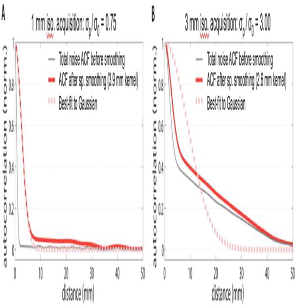
Simulations depict two strategies to achieve the same final spatial resolution (4 mm). We generated synthetic time-series noise consisting of a thermal noise component and a physiological noise component. The synthetic thermal noise component was white-noise by design and therefore its spatial autocorrelation function is a Gaussian with a one-pixel FWHM. The physiological noise component was synthesized to have strong spatial autocorrelation out to 40 mm FWHM. These two sources were combined with weightings reflecting the σ_p/σ₀ ratios seen in common fMRI acquisitions. The two strategies toward achieving the same final spatial resolution fMRI map were compared. (A) Acquire small voxels (1 mm isotropic) and spatially smooth to 4 mm. For 3T 32-channel coil acquisitions this is expected to be firmly thermal noise-dominated at acquisition. A thermal/physiological ratio of σ_p/σ₀ = 0.75 and Gaussian smoothing kernel of 3.87 mm were used. (B) Acquire conventionally-sized voxels (3 mm isotropic) and smooth to 4 mm. In this case the acquisition is firmly physiologically noise dominated for the 32-channel coil at 3T. The measured thermal/physiological ratio σ_p/σ₀ = 3.0 and Gaussian smoothing kernel of 2.65 mm were used.

Even though both acquisition/smoothing strategies were chosen to result in the same final spatial resolution (4 mm), only the strategy used in A (high spatial resolution, thermal noise dominated acquisition) results in a final ACF (solid red line) that is well described by a Gaussian function (best-fit Gaussian is shown in dashed red line). The strategy used in B (conventional resolution acquisition dominated by physiological noise) results in an ACF that deviates strongly from Gaussian, especially in the tails of the distribution, due to the long-range spatial correlations seen in physiological noise.

Conclusions

Here we have considered hardware and acquisition choices impact the physiological to thermal noise ratio, σ_p/σ_0. We suggest that this figure of merit for the acquisition informs the practitioner about the assumptions made by standard fMRI analysis techniques. We have focused on analysis using Random Field Theory in part because it is a well-known method that (today) is used by the vast majority of practitioners, but also to respond to the very recent Eklund et al. article that has already generated a large amount of discussion within the field.[Eklund et al 2016] One of the conclusions of the Eklund et al. study is that because nonparametric permutation tests do not make the same assumptions of Gaussianity as Randon Field Theory they do not suffer from this save inflated FPR problem and are “valid for any spatial autocorrelation function”. However, the permutation test approach is not without its own limitations and may not be as universally applicable as Random Field Theory (as reviewed by Flandin & Friston, 2016 [Flandin & Friston 2016]) when the assumptions of Random Field Theory are met.

Maintaining thermal noise dominance is the principle acquisition strategy that can assure that the noise model used in parametric analysis packages reflects reality (and therefore generates accurate FPRs in cluster-wise inferences). At sufficiently low values of σ_p/σ₀, the time-series noise is Gaussian-distributed is therefore accurately described by the noise model assumed in parametric tests. Here we reviewed the literature describing how σ_p/σ₀ < 1 can be achieved at high spatial resolution, especially if highly accelerated imaging is used. To achieve this, the spatial resolution must be increased considerably from that of the “1000 functional connectomes” data set (Biswal et al., 2010) which formed the basis of the Eklund et al. study.

For applications where high spatial resolution is not intrinsically valuable, we assess the strategy of acquiring at high spatial resolution (which causes the data to be thermal noise dominated) and smoothing to the desired spatial resolution. Anatomically informed smoothing, such as surface-based smoothing, can be employed to cancel uncorrelated thermal noise while avoiding signal contamination from nearby CSF or signal dilution from nearby white matter [Błażejewska et al. 2016] and to avoiding spatial localization errors stemming from, e.g., blurring together fMRI data from opposing banks of a sulcus.[Kiebel et al 2000, Andrade et al 2001) It appears that this strategy might be useful for controlling the heavy tails in the spatial ACF identified as the source of the false-positive rate problem in cluster-wise parametric analysis. We caution, however, that this strategy should be fully validated in a large-scale study using real acquisition data.

Highlights.

• Acquisition and hardware factors have a strong effect on the thermal and physiological noise components of the time-series noise in the fMRI experiment.

• Understanding the noise mixture and appropriately setting acquisition parameters is critical, since some noise components contain long-range spatial correlations implicated in biasing statistical inference.

References

- Andrade A, Kherif F, Mangin JF, Worsley KJ, Paradis AL, Simon O, Dehaene S, Le Bihan D, Poline JB. Detection of fMRI activation using cortical surface mapping. Human brain mapping. 2001;12(2):79–93. doi: 10.1002/1097-0193(200102)12:2<79::AID-HBM1005>3.0.CO;2-I. [DOI] [PMC free article] [PubMed] [Google Scholar]
- Birn RM, Smith MA, Jones TB, Bandettini PA. The respiration response function: the temporal dynamics of fMRI signal fluctuations related to changes in respiration. Neuroimage. 2008;40(2):644–654. doi: 10.1016/j.neuroimage.2007.11.059. [DOI] [PMC free article] [PubMed] [Google Scholar]
- Biswal BB, Mennes M, Zuo XN, Gohel S, Kelly C, Smith SM, Beckmann CF, Adelstein JS, Buckner RL, Colcombe S, Dogonowski AM, Ernst M, Fair D, Hampson M, Hoptman MJ, Hyde JS, Kiviniemi VJ, Kotter R, Li SJ, Lin CP, Lowe MJ, Mackay C, Madden DJ, Madsen KH, Margulies DS, Mayberg HS, McMahon K, Monk CS, Mostofsky SH, Nagel BJ, Pekar JJ, Peltier SJ, Petersen SE, Riedl V, Rombouts SA, Rypma B, Schlaggar BL, Schmidt S, Seidler RD, Siegle GJ, Sorg C, Teng GJ, Veijola J, Villringer A, Walter M, Wang L, Weng XC, Whitfield-Gabrieli S, Williamson P, Windischberger C, Zang YF, Zhang HY, Castellanos FX, Milham MP. Toward discovery science of human brain function. Proc Natl Acad Sci U S A. 2010;107:4734–4739. doi: 10.1073/pnas.0911855107. [DOI] [PMC free article] [PubMed] [Google Scholar]
- Błażejewska A, Hinds OP, Polimeni JR. Improved tSNR of high-resolution fMRI with surface-based cortical ribbon smoothing. Annual Meeting of the Organization for Human Brain Mapping. 2016:1728. [Google Scholar]
- Bodurka J, Ye F, Petridou N, Murphy K, Bandettini PA. Mapping the MRI voxel volume in which thermal noise matches physiological noise–implications for fMRI. Neuroimage. 2007;34:542–549. doi: 10.1016/j.neuroimage.2006.09.039. [DOI] [PMC free article] [PubMed] [Google Scholar]
- Britz J, Van De Ville D, Michel CM. BOLD correlates of EEG topography reveal rapid resting-state network dynamics. NeuroImage. 2010;52(4):1162–70. doi: 10.1016/j.neuroimage.2010.02.052. [DOI] [PubMed] [Google Scholar]
- Chang C, Cunningham JP, Glover GH. Influence of heart rate on the BOLD signal: the cardiac response function. NeuroImage. 2009;44(3):857–69. doi: 10.1016/j.neuroimage.2008.09.029. [DOI] [PMC free article] [PubMed] [Google Scholar]
- Dagli MS, Ingeholm JE, Haxby JV. Localization of cardiac-induced signal change in fMRI. NeuroImage. 1999;9(4):407–15. doi: 10.1006/nimg.1998.0424. [DOI] [PubMed] [Google Scholar]
- de Zwart JA, van Gelderen P, Golay X, Ikonomidou VN, Duyn JH. Accelerated parallel imaging for functional imaging of the human brain. NMR Biomed. 2006;19:342–351. doi: 10.1002/nbm.1043. [DOI] [PubMed] [Google Scholar]
- Eklund A, Nichols TE, Knutsson H. Cluster failure: Why fMRI inferences for spatial extent have inflated false-positive rates. Proc Natl Acad Sci U S A. 2016;113:7900–7905. doi: 10.1073/pnas.1602413113. [DOI] [PMC free article] [PubMed] [Google Scholar]
- Enzmann DR, Pelc NJ. Brain motion: measurement with phase-contrast MR imaging. Radiology. 1992;185(3):653–60. doi: 10.1148/radiology.185.3.1438741. [DOI] [PubMed] [Google Scholar]
- Flandin G, Friston KJ. Analysis of family-wise error rates in statistical parametric mapping using random field theory. 2016 doi: 10.1002/hbm.23839. arXiv:1606.08199 [stat.AP] [DOI] [PMC free article] [PubMed] [Google Scholar]
- Glover GH, Li TQ, Ress D. Image-based method for retrospective correction of physiological motion effects in fMRI: RETROICOR. Magnetic Resonance in Medicine. 2000;44(1):162–7. doi: 10.1002/1522-2594(200007)44:1<162::aid-mrm23>3.0.co;2-e. [DOI] [PubMed] [Google Scholar]
- Gonzalez-Castillo J, Roopchansingh V, Bandettini PA, Bodurka J. Physiological noise effects on the flip angle selection in BOLD fMRI. NeuroImage. 2011;54(4):2764–78. doi: 10.1016/j.neuroimage.2010.11.020. [DOI] [PMC free article] [PubMed] [Google Scholar]
- Greitz D, Franck A, Nordell B. On the pulsatile nature of intracranial and spinal CSF-circulation demonstrated by MR imaging. Acta radiologica (Stockholm, Sweden : 1987) 1993;34(4):321–8. [PubMed] [Google Scholar]
- Griswold MA, Jakob PM, Heidemann RM, Nittka M, Jellus V, Wang J, Kiefer B, Haase A. Generalized autocalibrating partially parallel acquisitions (GRAPPA) Magn Reson Med. 2002;47:1202–1210. doi: 10.1002/mrm.10171. [DOI] [PubMed] [Google Scholar]
- Hu X, Le TH, Parrish T, Erhard P. Retrospective estimation and correction of physiological fluctuation in functional MRI. Magnetic Resonance in Medicine. 1995;34(2):201–12. doi: 10.1002/mrm.1910340211. [DOI] [PubMed] [Google Scholar]
- Hutton C, Balteau E, Lutti A, Josephs O, Weiskopf N. Modelling temporal stability of EPI time series using magnitude images acquired with multi-channel receiver coils. PLoS One. 2012;7:e52075. doi: 10.1371/journal.pone.0052075. [DOI] [PMC free article] [PubMed] [Google Scholar]
- Kellman P, McVeigh ER. Image reconstruction in SNR units: a general method for SNR measurement. Magn Reson Med. 2005;54:1439–1447. doi: 10.1002/mrm.20713. [DOI] [PMC free article] [PubMed] [Google Scholar]
- Kiebel SJ, Goebel R, Friston KJ. Anatomically informed basis functions. NeuroImage. 2000;11(6 Pt 1):656–67. doi: 10.1006/nimg.1999.0542. [DOI] [PubMed] [Google Scholar]
- Klose U, Strik C, Kiefer C, Grodd W. Detection of a relation between respiration and CSF pulsation with an echoplanar technique. Journal of magnetic resonance imaging : JMRI. 2000;11(4):438–44. doi: 10.1002/(sici)1522-2586(200004)11:4<438::aid-jmri12>3.0.co;2-o. [DOI] [PubMed] [Google Scholar]
- Kruger G, Glover GH. Physiological noise in oxygenation-sensitive magnetic resonance imaging. Magn Reson Med. 2001;46:631–637. doi: 10.1002/mrm.1240. [DOI] [PubMed] [Google Scholar]
- Larkman DJ, Hajnal JV, Herlihy AH, Coutts GA, Young IR, Ehnholm G. Use of multicoil arrays for separation of signal from multiple slices simultaneously excited. J Magn Reson Imaging. 2001;13:313–317. doi: 10.1002/1522-2586(200102)13:2<313::aid-jmri1045>3.0.co;2-w. [DOI] [PubMed] [Google Scholar]
- Mayhew JE, Askew S, Zheng Y, Porrill J, Westby GW, Redgrave P, Rector DM, Harper RM. Cerebral vasomotion: a 0.1-Hz oscillation in reflected light imaging of neural activity. NeuroImage. 1996;4(3 Pt 1):183–93. doi: 10.1006/nimg.1996.0069. [DOI] [PubMed] [Google Scholar]
- Moeller S, Yacoub E, Olman CA, Auerbach E, Strupp J, Harel N, Ugurbil K. Multiband multislice GE-EPI at 7 tesla, with 16-fold acceleration using partial parallel imaging with application to high spatial and temporal whole-brain fMRI. Magn Reson Med. 2010;63:1144–1153. doi: 10.1002/mrm.22361. [DOI] [PMC free article] [PubMed] [Google Scholar]
- Mumford J, Pernet C, Yeo T, Nickerson L, Muhlert N, Stikov N, Gollub R. Keep calm and scan on. Organization for Human Brain Mapping; Brain Mapping 2016 [Google Scholar]
- Poncelet BP, Wedeen VJ, Weisskoff RM, Cohen MS. Brain parenchyma motion: measurement with cine echo-planar MR imaging. Radiology. 1992;185(3):645–51. doi: 10.1148/radiology.185.3.1438740. [DOI] [PubMed] [Google Scholar]
- Pruessmann KP, Weiger M, Scheidegger MB, Boesiger P. SENSE: sensitivity encoding for fast MRI. Magn Reson Med. 1999;42:952–962. [PubMed] [Google Scholar]
- Raj D, Anderson AW, Gore JC. Respiratory effects in human functional magnetic resonance imaging due to bulk susceptibility changes. Physics in medicine and biology. 2001;46(12):3331–40. doi: 10.1088/0031-9155/46/12/318. [DOI] [PubMed] [Google Scholar]
- Renvall V, Nangini C, Hari R. All that glitters is not BOLD: inconsistencies in functional MRI. Scientific Reports. 2014;4(3920):1–8. doi: 10.1038/srep03920. [DOI] [PMC free article] [PubMed] [Google Scholar]
- Roemer PB, Edelstein WA, Hayes CE, Souza SP, Mueller OM. The NMR phased array. Magn Reson Med. 1990;16:192–225. doi: 10.1002/mrm.1910160203. [DOI] [PubMed] [Google Scholar]
- Setsompop K, Gagoski BA, Polimeni JR, Witzel T, Wedeen VJ, Wald LL. Blipped-controlled aliasing in parallel imaging for simultaneous multislice echo planar imaging with reduced g-factor penalty. Magn Reson Med. 2012;67:1210–1224. doi: 10.1002/mrm.23097. [DOI] [PMC free article] [PubMed] [Google Scholar]
- Soellinger M, Rutz AK, Kozerke S, Boesiger P. 3D cine displacement-encoded MRI of pulsatile brain motion. Magnetic Resonance in Medicine. 2009;61(1):153–62. doi: 10.1002/mrm.21802. [DOI] [PubMed] [Google Scholar]
- Triantafyllou C, Hoge RD, Krueger G, Wiggins CJ, Potthast A, Wiggins GC, Wald LL. Comparison of physiological noise at 1.5 T, 3 T and 7 T and optimization of fMRI acquisition parameters. Neuroimage. 2005;26:243–250. doi: 10.1016/j.neuroimage.2005.01.007. [DOI] [PubMed] [Google Scholar]
- Triantafyllou C, Hoge RD, Wald LL. Effect of spatial smoothing on physiological noise in high-resolution fMRI. Neuroimage. 2006;32:551–557. doi: 10.1016/j.neuroimage.2006.04.182. [DOI] [PubMed] [Google Scholar]
- Triantafyllou C, Polimeni JR, Keil B, Wald LL. Coil-to-coil physiological noise correlations and their impact on functional MRI time-series signal-to-noise ratio. Magn Reson Med. 2016 doi: 10.1002/mrm.26041. [DOI] [PMC free article] [PubMed] [Google Scholar]
- Triantafyllou C, Polimeni JR, Wald LL. Physiological noise and signal-to-noise ratio in fMRI with multi-channel array coils. Neuroimage. 2011;55:597–606. doi: 10.1016/j.neuroimage.2010.11.084. [DOI] [PMC free article] [PubMed] [Google Scholar]
- Van de Moortele PF, Pfeuffer J, Glover GH, Ugurbil K, Hu X. Respiration-induced B0 fluctuations and their spatial distribution in the human brain at 7 Tesla. Magnetic Resonance in Medicine. 2002;47(5):888–95. doi: 10.1002/mrm.10145. [DOI] [PubMed] [Google Scholar]
- Wise RG, Ide K, Poulin MJ, Tracey I. Resting fluctuations in arterial carbon dioxide induce significant low frequency variations in BOLD signal. NeuroImage. 2004;21(4):1652–64. doi: 10.1016/j.neuroimage.2003.11.025. [DOI] [PubMed] [Google Scholar]
- Yan CG, Craddock RC, Zuo XN, Zang YF, Milham MP. Standardizing the intrinsic brain: towards robust measurement of inter-individual variation in 1000 functional connectomes. Neuroimage. 2013;80:246–262. doi: 10.1016/j.neuroimage.2013.04.081. [DOI] [PMC free article] [PubMed] [Google Scholar]
- Yuan H, Zotev V, Phillips R, Drevets WC, Bodurka J. Spatiotemporal dynamics of the brain at rest–exploring EEG microstates as electrophysiological signatures of BOLD resting state networks. NeuroImage. 2012;60(4):2062–72. doi: 10.1016/j.neuroimage.2012.02.031. [DOI] [PubMed] [Google Scholar]
- Zhao X, Bodurka J, Jesmanowicz A, Li SJ. B(0)-fluctuation-induced temporal variation in EPI image series due to the disturbance of steady-state free precession. Magnetic resonance in medicine. 2000;44(5):758–65. doi: 10.1002/1522-2594(200011)44:5<758::aid-mrm14>3.0.co;2-g. [DOI] [PubMed] [Google Scholar]