A graphical simulation model of the entire DNA process associated with the analysis of short tandem repeat loci

Abstract

The use of expert systems to interpret short tandem repeat DNA profiles in forensic, medical and ancient DNA applications is becoming increasingly prevalent as high-throughput analytical systems generate large amounts of data that are time-consuming to process. With special reference to low copy number (LCN) applications, we use a graphical model to simulate stochastic variation associated with the entire DNA process starting with extraction of sample, followed by the processing associated with the preparation of a PCR reaction mixture and PCR itself. Each part of the process is modelled with input efficiency parameters. Then, the key output parameters that define the characteristics of a DNA profile are derived, namely heterozygote balance (Hb) and the probability of allelic drop-out p(D). The model can be used to estimate the unknown efficiency parameters, such as π_extraction. ‘What-if’ scenarios can be used to improve and optimize the entire process, e.g. by increasing the aliquot forwarded to PCR, the improvement expected to a given DNA profile can be reliably predicted. We demonstrate that Hb and drop-out are mainly a function of stochastic effect of pre-PCR molecular selection. Whole genome amplification is unlikely to give any benefit over conventional PCR for LCN.

INTRODUCTION

In forensic, ancient DNA and some medical diagnostic applications, there may be limited, highly degraded DNA available (<100 pg) for analysis. To maximize the chance of a result, sufficient PCR cycles must be used to ensure that a single template molecule will be visualized. The universally accepted preferred method to analyse crime samples is with short tandem repeat (STR) DNA (1–3). However, there are two main problems that result from stochastic events: one or more alleles of a heterozygous individual may be completely absent, this is known as allele drop-out (4); in addition, PCR-generated slippage mutations or stutters (5) may be generated. Both events may compromise interpretation. In relation to analysis of ancient DNA, such as museum specimens or faeces of free-ranging animals, Taberlet et al. (6) used a computer simulation to address the question to determine the number of typing experiments needed to obtain a reliable result. These principles were adopted by Gill et al. (4), in conjunction with an extended statistical theory, to address similar issues that related to analysis of forensic samples. In forensic applications, there is also the added complication that the sample itself may be a mixture from two or more individuals. A number of statistical methods have been devised to aid interpretation. The first methods were based on the binary absence/presence of alleles (7). Later methods subsequently incorporated electropherogram peak height and area into programmed expert systems (8,9). In parallel to improvements of interpretation, the sensitivity of analysis has also improved to the extent that products of a single cell can be visualized, either by increased PCR cycle number (10) or by using novel individual cell-selection methods, such as laser microdissection (LMD) (11).

To improve understanding of the dependencies of parameters associated with DNA analysis, we provide a formal statistical model along with a computer implementation (PCRSIM) that simulates the entire process starting from: extraction → aliquot into pre-PCR reaction mixture → PCR amplification for t cycles → visualization of alleles after electrophoresis. We use Monte-Carlo simulation techniques to model the expected variation in PCR stutter artefacts, heterozygote balance (Hb), and to predict drop-out rates. Wherever possible, we also provide a formal statistical model. In addition, we also show how experimental data can be used to predict input parameters, such as extraction efficiency, by iteration to minimizing residuals to provide ‘best fit’ parameters. PCRSIM is therefore an all encompassing predictive model that describes the entire DNA process from the start to finish. As suggested by Stolovitzky and Cecchi (12), we use binomial distributions to model each step of the process. The parameter of the distributions is n, the number of template molecules. A template molecule has a probability π_extraction efficiency of extraction, π_aliquot of being in the aliquot taken and π_PCReff of surviving a PCR cycle. π_PCReff represents the efficiency of the PCR process in each cycle. As this paper relies heavily on the binomial distribution, it is worth stating the assumptions of the binomial model in relation to the problem at hand. The binomial distribution is used to model probability of observing x, the number of ‘successes’ in a set of n Bernoulli trials. The distribution uses only the number of successes, and not the order in which they occurred. There are four assumptions that must hold for the Binomial model to be valid. They are

1. There are a fixed number of trials: n is the number of template molecules, which is fixed by the amount of DNA in the sample.

2. There are only two possible outcomes in a trial, ‘success’ or ‘failure’. The outcomes are dependent on the stage of the process, but each stage has only two outcomes: extracted/not extracted; included/not included in aliquot; amplified/not amplified in each cycle of PCR; stutter/did not stutter on a particular PCR cycle.

3. The probability of a ‘success’ is constant for every trial. The probability of success in each stage is held constant in the model.

4. The trials are independent of one another. As we have used a binomial model, we have implicitly made the assumption of independence between individual template molecules. This seems reasonable, since the extraction process completely disrupts the integrity between individual chromosomes.

Other mathematical models to describe STR mutation slippage or stutter mutations during PCR have also been developed (13–15). These models simulated the PCR process using two stochastic processes: the first replicated template DNA sequences; the second reproduced slippage (stutter) mutations. Random binary trees were used to describe probabilistic relationships (using a different model to that presented here). However, these models were proposed in relation to dimeric microsatellites, which are inherently difficult to interpret as PCR slippage mutations or stutters (5) and occur at relatively high frequency at these loci. This results in ladder-type patterns where the actual allele may be at lower intensity than one of the stutter bands. Furthermore, a stutter mutation can either result in contraction or in expansion of the original stutter artefact. Mathematical methods have been developed (16) to deconvolve stutters from dimeric loci using experimental output data to inform probabilistic models. Because of the interpretational difficulties associated with dimeric loci, the forensic community has implemented tetrameric loci instead [reviewed in (3)]. These are much easier to interpret because the efficiency of stutter slippage during PCR is much lower and only a single band, 4 bp lower than the parent allele, is observed. Generally, the peak height/area is <10% the size of the parent allele (17). Consequently, our modelling requirements are much simplified as we only need to simulate the probability of conversion of band n_A→S_A using a binomial distribution Bin(n_A, π_stutter) to describe the number of new stutter molecules generated during each PCR cycle. In addition, we model only contraction of the allele, since expansions are not observed (or are too rare to visualize). π_stutter is ∼400 times less than π_PCReff. Once a stutter band has formed, then its replication during subsequent PCR cycles progresses exponentially with the same efficiency as for the parent allele, modelled by Bin(n_A, π_PCReff). It is important to understand the characteristics of stutters as they can compromise the interpretation of mixtures, where the minor contributor may have alleles of similar sizes to stutter bands of the major contributor.

Although previous authors (6) have modelled parts of the DNA process, none of them has described the entire process by computer simulation. To do this, we have first simulated each part of the DNA process, and then used a graphical model or Bayes Net solution to combine the parts. Each part of the process is represented by a node in the graphical model; each node comprises parameters and a distribution and is dependent upon other nodes in the model. Modelling processes in this way is intuitive and simplifies the complex inter-dependencies that are inherent in the multiple stochastic events that occur throughout the process of DNA analysis. We demonstrate that graphical models can be used to assess and measure unknown variables, such as sample extraction efficiency, or to optimize parameters, such as the amount of pre-PCR aliquot taken. By modelling ‘what-if’ scenarios, we can therefore improve entire DNA processes as a result, and this translates into improved success rates when real samples are analysed.

MATERIALS AND METHODS

DNA extraction and quantification

DNA was extracted using Qiagen™ QiaAmp Mini-Kits (Catalogue no. 51306) or Qiagen™ Genomic-Tip system (Catalogue no. 10223, 20/G tips). Samples had been stored frozen at −20°C and were defrosted at room temperature prior to DNA extraction. The manufacturers' protocol for each sample type was used to obtain between 0 and 2 ng/μl DNA (Mini-Kits) or between 5 and 15 ng/μl DNA (Genomic-Tips), suspended in 1× TE Buffer (ABD). Samples were quantified using Picogreen (18) and/or the Biochrom UV spectrophotometer (19). We also carried out real-time PCR quantification using the Applied Biosystems (Foster City, CA) Quantifiler Human kit™ and Quantifiler Y kit™ TaqMan assays, following the manufacturers' protocols (http://docs.appliedbiosystems.com/pebiodocs/04344790.pdf).

SGM plus™ PCR amplification

The method by Cotton et al. (20) was followed: AMPFISTR^® SGMplus™ kit (Applied Biosystems) containing reaction mixture, primer mixture (for components see PerkinElmer user manual), AmpliTaq Gold^® DNA polymerase at 5 U/μl and AMPFISTR^® control DNA, heterozygous for all loci in 0.05% sodium azide and buffer was used for the amplification of STR loci. DNA extract was amplified in a total reaction volume of 50 μl without mineral oil on a 9600 thermal cycler (Applied Biosystems GeneAmp PCR system) using the following conditions: 95°C for 11 min, 28 cycles [or 34 cycles for low copy number (LCN) amplification] of 94°C for 60 s, 59°C for 60 s, 72°C for 60 s; 60°C extension for 45 min; holding at 4°C.

Sample data from the 377 instrument was analysed using ABI Prism™ Genescan™ Analysis v3.7.1 and ABI Prism™ Genotyper™ software v3.7 NT. Data extracted from Genotyper™ (peak height, peak area, scan number and size in bases).

LMD

The method by Elliot et al. (11) was used to select N sperm or epithelial cells from microscope slides.

The theory of the simulation model

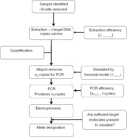
The simulation model mirrors current casework analysis using the Applied Biosystems second generation multiplex (SGMplus™) system (2,20) that is currently used in the majority of casework in the UK and elsewhere (Figure 1).

Figure 1.

An explanation of the DNA process.

Samples are typically purified using Qiagen columns (QIAamp DNA minikit; Qiagen, Hilden, Germany). A small aliquot (2 μl) of the purified DNA extract is then quantified using a method, such as the picogreen assay (19); then a portion is removed to carry out PCR. Dependent upon the casework assessment, coupled with information about the quantity of DNA present, a decision is made whether to analyse using 28 cycles (conventional: >250 pg in the total PCR reaction) or whether LCN protocols are followed (4), using 34 PCR cycles if <250 pg and/or the DNA is highly degraded. After PCR, the samples are electrophoresed using AB 377 instrumentation. Genotyping is automated using Genescan, and Genotyper software. Allele designation is carried out with the help of expert systems ‘STRESS’ (21) and ‘True Allele’ (Cybergenetics, Pittsburgh, http://www.cybgen.com/. If mixtures are present, then an expert system PENDULUM (8,22) is used to devolve genotype combinations.

Parameter estimation

PCRSIM is a prototype computer program, based upon the theory described in this paper. The program attempts to explicitly model the DNA extraction and PCR processes at the molecular level. The model can be defined by a series of input and output parameters as follows:

Input parameters

1. No. of cells (N): Typically a stain or sample will contain N cells. Each diploid DNA cell comprises ∼6 pg of DNA (23) and a haploid cell comprises 3 pg DNA. Given a DNA concentration, it is possible to convert this into an equivalent number of haploid or diploid cells.

2. Extraction efficiency (π_extraction): During the process of extraction, the cells are disrupted and the DNA liberated into solution. During extraction, there is a probability π_extraction (the extraction efficiency) that a given DNA molecule will survive the process.

3. Aliquot (π_aliquot): A portion of the extracted sample is submitted for PCR. Therefore, there is a probability π_aliquot, 0 < π_aliquot < 1, that a given molecule will be selected.

4. PCR efficiency (π_PCReff): PCR is not 100% efficient; hence, during each round there will be a finite probability π_PCReff that a DNA fragment will be amplified.

5. No. of PCR cycles (t): Typically t = 28 for normal DNA profiling and t = 34 cycles for LCN.

Output parameters

1. Probability of allele drop-out, p(D): The chance that an allele will fail to amplify.

2. Number of amplified molecules (n_A, n_B): The simulated number of molecules for a given allele A or B can be measured and compared against threshold level T that must be achieved in order for a signal to be observed (this is ∼4 × 10⁵/μl of PCR amplification product). Note for 34 cycle PCR T is always achieved

3. Heterozygote balance: For a given heterozygote locus, we derive a distribution of $Hb=min\left[n_A\left(t\right),n_B\left(t\right)\right]/max\left[n_A\left(t\right),n_B\left(t\right)\right]$.

RESULTS

Description of the process

PCRSIM simulates the biochemical processes that are used to process a DNA sample (Figure 1). Taberlet et al. (6) originally assessed the chance of observing both alleles of a heterozygote relative to the number of pre-PCR template molecules for diploid cells. We extend the discussion here; first, we do not make the assumption that for a given heterozygote there are equivalent numbers of both alleles in the pre-PCR reaction mixture; second, we present a formal statistical model that simplifies the computational aspects.

Extraction efficiency

Typically, the Qiagen method of extraction is used. This involves the addition of chaotropic salts to an extract of a body fluid and subsequent purification using a silica column. At the end of the process, purified DNA is recovered. Unfortunately, some of the DNA is lost during the process and is therefore unavailable for PCR. The parameter π_extraction describes the extraction efficiency. For example, if n target DNA molecules are extracted with π_extraction = 0.5, then on average approximately n/2 molecules are recovered.

The extraction process can be modelled using a binomial distribution with parameters 2N and π_extraction. If we simulated 1000 times the extraction process with 10 diploid cells (N = 10) and π_extraction = 0.6, then we would expect to see on average between 5 and 18 copies of recovered DNA template per locus.

In practice, an aliquot will be forwarded for PCR amplification, which enables repeat analysis if required. Typically, out of a total extract of 66 μl, a portion of 20 μl will be forwarded for PCR. The selection of template molecules by pipetting can also be modelled using another binomial distribution of the form Bin(n, π_aliquot), where π_aliquot = 20/66 (the aliquot proportion). The 20 μl extract is then forwarded into a PCR reaction mixture to make a total 50 μl. At least 20 cells are needed to avoid allele drop-out. If five cells are extracted, then on average 35% of heterozygous loci will exhibit allele drop-out.

PCR amplification

PCR does not occur with 100% efficiency. The amplification efficiency (π_PCReff) can range between zero and one. The process can be described by π_PCReff (24), where n_t is the number of amplified molecules, n₀ is the initial input number of molecules and t is the number of amplification cycles. However, a strictly deterministic function will not model the errors in the system, especially if we are interested in LCN estimations (e.g. <20 target copies).

We have modelled PCR amplification using a function of the binomial distribution. The first round PCR replicates the available template molecules per locus (n₀) with efficiency π_PCReff to produce n₁ new molecules per locus:

$$n_1=n_0+Bin\left(n_0,{\pi }_{\text{PCReff}}\right)$$

For the second round of PCR, both n₀ and n₁ are available hence:

$$n_2=n_1+Bin\left(n_1,{\pi }_{\text{PCReff}}\right)$$

If there are t PCR cycles, then we can generalize that the final number of molecules generated per locus is:

$$n_t=n_{t-1}+Bin\left(n_{t-1},{\pi }_{\text{PCReff}}\right)$$

where

$$n_{t-1}={\displaystyle \sum _{i=1}^{t-1}}{n}_i$$

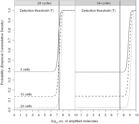
We simulate n_t 1000 times to estimate the variation. For LCN typing, there are typically t = 34 PCR cycles. This will enable a single target copy to be visualized, because it will always produce sufficient molecules to exceed the detection threshold (T), i.e. >2 × 10⁷ molecules in the total of 50 μl PCR reaction (Figure 2) or ∼4 × 10⁵ per μl of amplified DNA. Single cells can be visualized (10). We can generalize that for 34 cycle PCR, the phenomenon of drop-out is dominated solely by the absence of template in the pre-PCR mixture, predicted levels of drop-out pre- and post-PCR are the same in Figure 2. However, if the number of PCR cycles is reduced to a level that does not produce sufficient copies to trigger the threshold level (T), then there will be a failure to detect, i.e. p(D) consist of two components:

$$p\left(D\right)=p\left(D_{\text{S}}\right)+p\left(D_T\right)$$

where p(D_s) is the pre-PCR stochastic element and p(D_T) = p(n_t < T).

Figure 2.

Cumulative probability density of 5, 10, 20 cells after extraction (π_extraction = 0.6), selection of an aliquot (π_aliquot = 20/66) and PCR (π_PCReff = 0.8) using 28 and 34 cycles, respectively. The threshold of detection (T) is ∼2 × 10⁷ molecules in the total PCR reaction mixture. At 34 cycles, if a single molecule is present in the aliquot, then it will be amplified and sufficient will be present to exceed the detection threshold. When number of amplified molecules = 0, this means drop-out has occurred. With five cells, this is ∼38%.

An algebraic solution for the pre-PCR probability of drop-out is given in Appendix 1 (Supplementary Material).

Experimental estimation of PCR efficiency π_PCReff

We used real-time PCR using a commercial Applied Biosystems Y-Quantifiler kit (25) to estimate quantities of DNA present. This method employs a 70 base Y chromosome fragment that is PCR amplified in real-time. A series of C_T values were calculated for 23–50 000 target copies (data not shown). The C_T value is the point measured in terms of PCR cycles, where the level of fluorescence exceeds the background noise (an arbitrary threshold). The more target molecules available, the fewer cycles required to reach C_T. From the regression of the C_T slope, we estimated π_PCReff = 10^[−1/slope] − 1 (24) and determined π_PCReff = 0.82(SE ± 0.12).

This also corresponded well to the estimate of π_PCReff found by minimizing the (observed − expected)² residuals from Hb output when known quantities of DNA were PCR amplified (data not shown). Throughout, we have used π_PCReff = 0.8.

Quantification

Quantification is carried out after DNA extraction and purification. A number of different methods can be utilized, e.g. pico-green assay (19). The purpose of quantification is to ensure that there are sufficient DNA molecules (n₀) in the PCR reaction mixture, so that after t amplification cycles n_t molecules are produced. The aim is to ensure that n_t > T. If n_t < T, then allele drop-out will occur because the signal is insufficient to be detected by the photomultiplier. Generally, when levels of DNA are <0.05 ng/μl, then estimates of quantity tend to be unreliable (26). However, newer methods based on real-time TaqMan assays (e.g. AB Quantifiler™ kit) (27) appear to offer much higher sensitivity and will in turn make the decision-making process more reliable. Alternatively, if too much DNA is applied then the electrophoretic system will be overloaded. Generally, multiplexed systems are optimized to analyse ∼250 pg to 1 ng DNA. Hence, in practice the quantification process is used to determine π_aliquot, which is therefore an operator-dependent variable ranging from 1 to 20 μl used to optimize n₀. The number of PCR cycles (t) is also a variable (either 28 or 34 cycles in our experiments) and this decision is also dependent upon an estimate of n₀. Quantification estimates the quantity (pg) of post-extracted DNA in a sample. There are ∼6 pg per cell nucleus (23); hence, we can estimate the equivalent number of (2n) target molecules that are input into the simulation model at the PCR stage.

Heterozygote balance

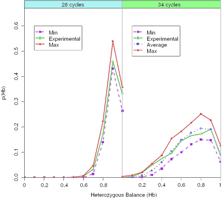
For a heterozygote locus with alleles A and B, for each allele we simulate 1000 times the number of post-PCR molecules n_A(t) and n_B(t). Given the two parameters π_aliquot and π_PCReff, we obtain 1000 estimates of Hb = min [n_A(t), n_B(t)]/[max n_A(t), n_B(t)]. Simulation results were compared with experimental data from 1692 heterozygotes from ∼1 ng of DNA. By experimenting with different values of n, we found that experimental data actually corresponded to a best fit of ∼500 pg DNA input into the pre-PCR reaction mixture. This is ∼83 diploid cells. In a recent collaborative study (26,28), it was demonstrated that after initial quantification, there was a significant loss of DNA with reported recovery of 53–84% (consistent with our results) explained by binding of DNA to the walls of plasticware. Reducing π_PCReff had very little effect on Hb. Our main interest was LCN DNA template (t = 34), where stochastic effects are marked, a choice of a single parameter for π_PCReff = 0.8 was shown to work well for all simulations; furthermore, we did not need to alter the assumption of n derived from quantification estimates. Provided that sufficient template was produced to trigger the threshold level T, then the model was relatively insensitive to changes in π_PCReff. Figure 3 demonstrated that there was very good agreement between the simulation and observed results. The results also provide a strong theoretical basis for the widely used guideline for the acceptable range of Hb, Hb ≥ 0.6 (17,29), which is used to assist interpretation of mixtures when optimal amounts of DNA are analysed.

Figure 3.

Simulations of Hb (1000×) of 500 pg (83 diploid cells), 28 PCR cycles and 25 pg (4 diploid cells), 34 PCR cycles, compared with experimental observations.

In the second experiment, we simulated 25 pg pre-PCR input (Figure 3). Hb becomes much more variable, although drop-out was not encountered. This also illustrated the importance of maximizing n₀ in the pre-PCR reaction; in previous experiments significant drop-out was encountered when five cells were diluted into 20/66 μl. Once again the simulation and experimental data gave a very good fit. This time, it was not necessary to iterate any of the input parameters, since at lower levels of DNA, the PCR amplification stayed in the log-linear phase throughout.

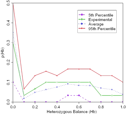
Finally, we modelled complex scenarios to demonstrate how to estimate parameters, such as π_extraction. LMD was used to select 10 epithelial cells. These were purified by Qiagen columns. The aliquot was π_aliquot = 20/66, and PCR was performed for 34 cycles (t = 34). Simulation proceeded by altering the input value π_extraction [note that the simulation was relatively insensitive to π_PCReff; provided that n_t > T, then p(D) was independent of π_PCReff]. By using different values of π_extraction, we showed that the differences between the observed and estimated distributions of Hb are minimized when π_extraction = 0.46. In addition, the difference between the observed drop-out probability p(D) and the simulated drop-out probability is simultaneously minimized. There is quite a high loss of DNA during extraction in this example, and demonstrates that the lower the amount of DNA that is purified, the less that can proportionately recovered by the Qiagen extraction methods (Figure 4).

Figure 4.

Hb and p(D), where 10 epithelial cells picked by LMD, were compared with 1000 simulations, where parameters π_extraction = 0.46, π_PCReff = 0.8 and π_aliquot = 20/66

Haploid cells

In the allele selection process, there is a difference between haploid (sperm) and diploid cells. Although a single diploid cell has each allele at a locus represented once (i.e. in equal proportions), this is not true for haploid cells. For example, if only one haploid cell is selected then just one allele can be visualized. The chance of selecting alleles A or B at a heterozygote locus is directly dependent upon the number of sperm cells analysed.

To calculate the chance of observing alleles A and B in a sample of n sperm cells at a heterozygous locus, we calculate the probability of observing at least one copy of allele A and at least one copy of observing allele B. Starting with n sperm cells, we observe at least one copy of both alleles at a heterozygous locus if we do not observe all sperm cells being either allele A or allele B. The probability of this is $1-p_A^n-p_B^n$. If p_A = p_B = 0.5 this probability is 1 − 0.5ⁿ⁻¹.

Therefore, the answer to the alternative question of how many sperm cells (n) are needed if we wish to be 100% confident that we will see both alleles (if the subject truly is heterozygous) is given by:

$$n=1+\frac{log(1-p)}{log\left(0.5\right)}.$$

This expression will not give integer values, so the recommended number would be the ceiling value of this expression. For example, if we wish to be 99% confident, then expression would return n = 7.64 (two decimal places), which we would round up to eight sperm cells. At least six sperm cells are required to be 95% certain.

This theoretical result is the best that possibly can be achieved under the assumption that a single allelic template can be detected in an extract. This relationship should work well for direct PCR methods. In practice, more sperm cells are required since extraction methods are inefficient and consequently DNA will be lost prior to PCR.

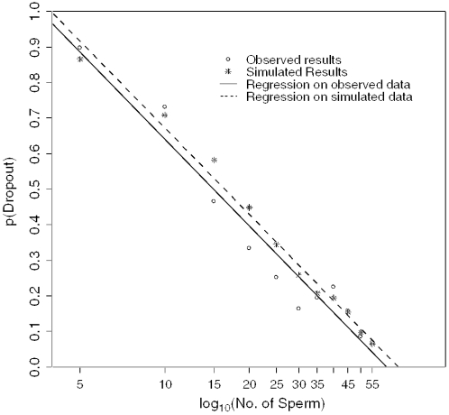
In a second experiment, we picked 1–55 sperm cells (N) from an individual of known genotype and analysed as described previously; plotting N versus observed p(D) we demonstrated a log-linear relationship. The best fit with the data is achieved when π_extraction = 0.3 (Figure 5). It can be seen from Figure 5 that the differences between the predicted and observed values are small, which indicates that the model is robust. At a practical level, it appears that the success rate for extracting sperm was much lower than for epithelial cells (Figure 4).

Figure 5.

Comparison of the number of sperm extracted versus observed probability of drop-out against a simulation using π_extraction = 0.3. There was no significant difference between regressions.

Evaluation of stutter

Stutters are artefactual bands that are produced by molecular slippage of the Taq polymerase enzyme (5). This causes an allelic band to alter its state from its parent, in vivo, state during successive amplifications. In dimeric STRs, there is a high probability π_stutter of stutter formation; hence, the parent can change state to S₁→S₂→S₃ and so on. This leads to a ladder formation of multiple stutters that can cause significant interpretation problems, especially if mixtures are encountered. Sometimes stutter formation exceeds that of the parent allele. Shinde et al. (14) have estimated π_stutter for (CA)_6–15 repeat sequences to range between 0.01 and 0.04 (increasing with the number of tandem repeats). The rate is even higher for (A)_n repeats, where π_stutter can reach 0.1. In contrast, for the more stable tetrameric loci, we estimated π_stutter = 0.002 which is at least an order of magnitude lower, consequently only one 4 bp stutter is encountered, usually <10% the size in peak height/area of the parent allele itself (17). Because they are easier to interpret, tetrameric STRs are universally used by forensic scientists in national DNA databases (2). Nevertheless, the presence of stutter may compromise some mixtures, especially where there are contributions from two individuals one of whom contributes more than twice as much DNA as the other. For this reason, it is important to model π_stutter.

We assess the chance π_stutter that Taq enzyme slippage leads to a stutter. This can happen only during PCR; hence, the number of stutter templates in the pre-PCR (n₀) reaction mixture is always zero.

Once a stutter is formed, then it acts as template identical to a normal allele (as the sequence is the same as an allele one repeat less than the parent). Consequently, the propagation of stutter is exponential with efficiency π_PCReff and after t cycles forms S_t stutter molecules. In the electropherogram, the quantity of stutter band is always measured relative to the parent allele:

$$p\left(S_A\right)=\frac{\phi S_A}{{\phi }_A}$$

where φ = peak area or peak height of the stutter (S_A) and allele (A), respectively. We refer to p(S_A) as the proportion of stutter. p(S_A) is not an estimate of π_stutter, but rather a by-product of π_stutter. In practice, ∼5% alleles fail to produce visible stutter, i.e. S_t < T.

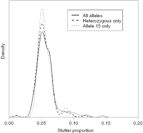
The relative peak area of stutter is variable between loci and also between alleles (14); therefore, it may be appropriate to evaluate stutter at every allelic position. In order to assess whether this, locus D3 from the SGM plus system was chosen and kernel density estimates of stutter peak areas were obtained:

1. Across all stutters regardless of whether the parent allele was homozygous or heterozygous.

2. When stutters were only associated with heterozygotes.

3. When stutters were associated with parent allele 15 only, i.e. at the allele 14 position.

Comparison showed there was little difference between the density estimates (Figure 6), although predictably, the subset of data that related specifically to allele 15 had multiple modes in the tail indicating sparsity of data in that region.

Figure 6.

Observed distribution of p(S) measured relative to (i) all alleles, (ii) heterozygotes only (iii) allele 15 only from 500 pg amplified target DNA.

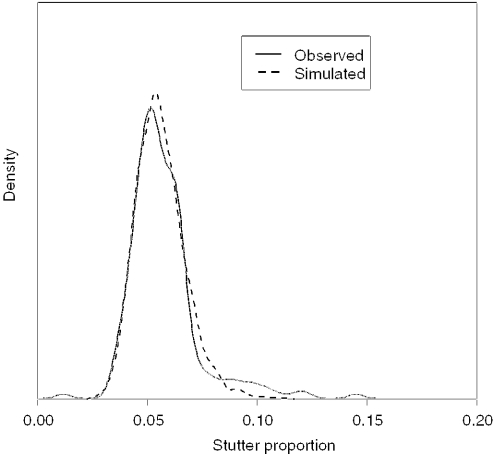
Based on all the D3 observations, π_stutter was modelled with a Beta distribution. The parameters of the Beta distribution were chosen so that, the distribution of π_stutter had a mean of ${\mu }_{{\pi }_{\text{stutter}}}=0.002$ and a variance of ${\sigma }_{{\pi }_{\text{stutter}}}^{\text{2}}=2.25\times {10}^{-6}$. This can be carried out by using the following identities: if X ∼ Beta(α,β), and E[X] = μ_X, SD(X)= σ_X, then $\alpha ={\mu }_X\left[{\mu }_X\left(1-{\mu }_x\right)/{\sigma }_X^2-1\right]$ and $\beta =\left(1-{\mu }_X\right)\left[{\mu }_X\left(1-{\mu }_x\right)/{\sigma }_X^2-1\right]$. For the given mean and variance this results in α = 1.77 and β = 884.34 (Figure 7). Recall that we determined that the minimized residuals were achieved when π_stutter = 0.002, which is an order of magnitude lower than the estimates for dimeric STRs (14).

Figure 7.

A comparison of the stutter from observed versus simulated distributions from 500 pg target DNA.

DISCUSSION

A graphical model to demonstrate the DNA PCR process

We have subdivided the DNA process (Figure 1) into a series of sub-processes that can individually be characterized by a series of input and output parameters. We demonstrated how parameters may be estimated using PCRSIM. To formalise our thinking and to provide a robust framework for modelling purposes, we present a graphical model (or Bayes Net) in Appendices 2 and 3 (Supplementary Material) (30). A graphical model consists of two major components, nodes (representing variables) and directed edges. A directed edge between two nodes, or variables, represents the direct influence of one variable on the other. To avoid inconsistencies, no sequences of directed edges which return to the starting node are allowed, i.e. a graphical model must be acyclic. Nodes are classified as either constant nodes or stochastic nodes. Constants are fixed by the design of the study: they are always founder nodes (i.e. they do not have parents). Stochastic nodes are variables that are given a distribution. Stochastic nodes may be children or parents (or both) (http://www.mrc-bsu.cam.ac.uk/bugs/). In pictorial representations of the graphical model, constant nodes are depicted as rectangles, stochastic nodes as circles.

This solution is appealing in the modelling of a complex stochastic system because it allows the ‘experts’ to concentrate on the structure of the problem before having to deal with the assessment of quantitative issues. It is also appealing in that the model can be easily modified to incorporate other contributing factors to the process, such as contamination (31). We provide a generalized model, but recognize that this can be continuously improved by modifying the nodes, e.g. PCR efficiency is itself a variable that decreases with molecular weight of the target sequence (32), but this relationship can also be easily modelled. π_PCReff is also affected by degradation where the high molecular weight material has preferentially degraded, but we envisage that the continued development of multiplexed real-time quantification assays (27) where PCR fragments of different sizes can be analysed will give a better indication of the degradation characteristics of the sample. Pre-casework assessment strategies informed by real-time PCR quantitative assays, such as the Applied Biosystems Quantifiler™ kit, combined with expert systems will remove much of the guess-work currently associated with DNA processing.

Use of the graphical model to simulate DNA profiles

Finally, we use the PCRSIM model to generate random DNA profiles from allelic frequency databases (33). Given the parameters that describe quantity and PCR efficiency, it is possible to simulate entire SGM plus profiles comprising 11 loci. At low quantities of DNA, stochastic effects result in partial DNA profiles. Consequently, each time a different PCR is carried out, each will give a different result. Either drop-out occurs or samples are very unbalanced within and between loci. Some researchers have attempted to improve systems by using alternative amplification methods. In particular, there is much interest in Whole Genome Amplification (34,35). However, we have demonstrated that the reasons for imbalance are predominantly stochastic, and not related to biochemistry. Provided that n_t > T, a theoretical basis to improve profile morphology by applying a novel enzymatic biochemistry does not seem to exist simply because the allelic imbalance is predominantly a function of the number of molecules present at the start (n₀).

Consequently, when there is limited DNA available, it is useful to produce entire simulated DNA profiles before the actual analysis is carried out. This assists the decision-making process to decide π_aliquot and the number of cycles (t) required to ensure n_t > T.

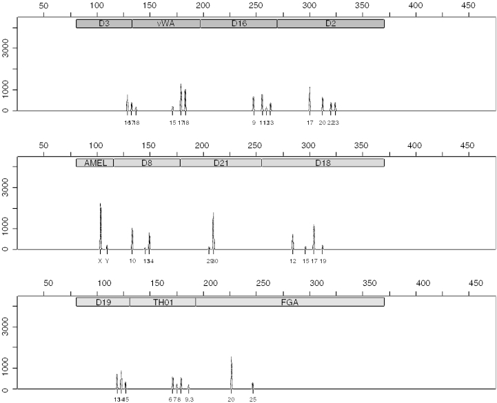
New methods of quantification that employ real-time PCR analysis (27) are much more accurate than those previously utilized (26); hence, this also greatly assists the pre-assessment process and does make the method more powerful, especially when estimating N, n and π_PCReff parameters. In addition, methods that specifically amplify a portion of the Y chromosome are important to give an indication of the quantity and quality of the male DNA. Combining the Applied Biosystems Quantifiler™ and Y-Quantifiler™ tests therefore provide an opportunity to separately assess the male/female mixture components before the main test is actually carried out. This is important because one of the biggest interpretational challenges is with mixtures (which are commonly encountered in forensics). Previous development of expert systems (8,16,21) are dependent upon a direct assessment of output data. Here, we have approached the problem in a completely different way. Rather than analyse the output data from the electropherogram, we produce a simulation model that includes input parameters n, N and π_PCReff and apply Monte-Carlo simulation in order to determine, in a probabilistic way, a range of results. This is a much more powerful approach than those previously described, simply because the output parameters that generate the distributions of Hb, n_t, p(D) and p(S) are crucially dependent upon the input parameters π_extraction, π_PCReff, n, N and t. However, once the output parameters are identified, they can then be used to improve other specialist expert systems that currently use these generalized parameters in their software. For example, to characterize mixtures, an algorithm called PENDULUM (8) is used, based upon residual least-squares theory (4). In this model, a series of heuristics are used to interpret low level DNA profiles and the parameters are fixed, but with PCRSIM we can now modify the parameters on a case-by-case basis and can import them into the final interpretation package (Figures 8–10).

Figure 8.

Simulation of SGM plus LCN-STR profiles from a mixture of 50 female cells and 20 male cells. PCR amplified 34 cycles. Counts of the y-axis were standardized by 2.35 × 10⁷ (T) and then scaled by 2 × 10⁶. Stutter module was not used in this simulation.

Figure 10.

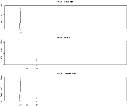
Simulated locus FGA showing separated male/female results from PCRSIM showing drop-out at allele 22.

PCRSIM can also be used to generate random mixtures for any number of individuals. For example, we generated simple LCN two person SGMplus male/female mixtures. The mixture proportion (Mx) of a male/female mixture, where there are n_male and n_female input DNA molecules, is defined as:

$$\text{Mx}=\frac{n_{\text{male}}}{n_{\text{male}}+n_{\text{female}}}.$$

We repeatedly simulated pairs of SGM plus profiles, using defined n parameters to simulate a defined Mx_input (which is the true mixture proportion) and then analysed the generated profiles with PENDULUM. The program was used to deconvolve the mixture back into the constituent contributors, ranking the first 500 results along with a density estimate of Mx_output.

Although the majority of data gave results that were easily interpreted, we were more interested to examine the behaviour of outliers in order to assess what may be reasonably expected during the course of casework, in other words, how much can a PENDULUM estimate of Mx be affected by stochastic variation?

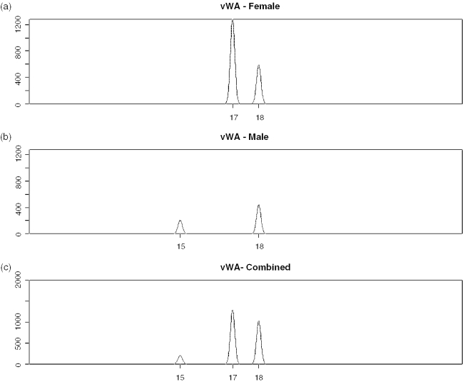
Consequently, we simulated 1000 male/female LCN mixtures, where Mx_input = 0.28 male. The most extreme example obtained (Figure 8) resulted in highly unbalanced loci, e.g. HUMVWA and HUMFIBRA/FGA (Figures 9 and 10), yet PENDULUM was still able to deconvolve the mixture into its constituent genotypes.

Figure 9.

Simulated locus vWA showing individual (a) female and (b) male profiles generated by PCRSIM and (c) how they combine together to produce an unbalanced mixture.

However, we give this simple example purely to illustrate that datasets produced by PCRSIM are very powerful to generate an unlimited amount of artificial, yet realistic, test data. By providing case-specific input and output parameters to create probability distributions, this can subsequently be used to test robustness and to improve the functionality of external expert systems, such as PENDULUM. An attempt to generate such data by conventional experimental means, by simultaneously varying all of the input parameters would not be feasible, or would be very time-consuming, since literally thousands of experiments would be required to cover all possible combinations of parameters. Therefore, we propose that computer simulation is a useful tool to speed some of the more onerous tasks associated with validation of a new method.

SUPPLEMENTARY MATERIAL

Supplementary Material is available at NAR Online.

REFERENCES

- 1.Werrett D.J. The National DNA Database. Forensic Sci. Int. 1997;88:33–42. [Google Scholar]
- 2.Martin P.D. National DNA databases: practice and practicability. A forum for discussion. Prog. Forensic Genet. 2004;10:1–8. [Google Scholar]
- 3.Gill P. Role of short tandem repeat DNA in forensic casework in the UK—past, present, and future perspectives. BioTechniques. 2002;32:366–368. doi: 10.2144/02322rv01. 370, 372, passim. [DOI] [PubMed] [Google Scholar]
- 4.Gill P., Whitaker J., Flaxman C., Brown N., Buckleton J. An investigation of the rigor of interpretation rules for STRs derived from less than 100 pg of DNA. Forensic Sci. Int. 2000;112:17–40. doi: 10.1016/s0379-0738(00)00158-4. [DOI] [PubMed] [Google Scholar]
- 5.Walsh P.S., Fildes N.J., Reynolds R. Sequence analysis and characterization of stutter products at the tetranucleotide repeat locus vWA. Nucleic Acids Res. 1996;24:2807–2812. doi: 10.1093/nar/24.14.2807. [DOI] [PMC free article] [PubMed] [Google Scholar]
- 6.Taberlet P., Griffin S., Goossens B., Questiau S., Manceau V., Escaravage N., Waits L.P., Bouvet J. Reliable genotyping of samples with very low DNA quantities using PCR. Nucleic Acids Res. 1996;24:3189–3194. doi: 10.1093/nar/24.16.3189. [DOI] [PMC free article] [PubMed] [Google Scholar]
- 7.Evett I.W., Buffery C., Willott G., Stoney D. A guide to interpreting single locus profiles of DNA mixtures in forensic cases. J. Forensic Sci. Soc. 1991;31:41–47. doi: 10.1016/s0015-7368(91)73116-2. [DOI] [PubMed] [Google Scholar]
- 8.Bill M., Gill P., Curran J., Clayton T., Pinchin R., Healy M., Buckleton J. PENDULUM: a guideline based approach to the interpretation of STR mixtures. Forensic Sci. Int. 2004;148:181–189. doi: 10.1016/j.forsciint.2004.06.037. [DOI] [PubMed] [Google Scholar]
- 9.Curran J., Gill P., Bill M.R. Interpretation of repeat measurement DNA evidence allowing for multiple contributors and population substructure. Forensic Sci. Int. 2004;148:47–53. doi: 10.1016/j.forsciint.2004.04.077. [DOI] [PubMed] [Google Scholar]
- 10.Findlay I., Taylor A., Quirke P., Frazier R., Urquhart A. DNA fingerprinting from single cells. Nature. 1997;389:555–556. doi: 10.1038/39225. [DOI] [PubMed] [Google Scholar]
- 11.Elliott K., Hill D.S., Lambert C., Burroughes T.R., Gill P. Use of laser microdissection greatly improves the recovery of DNA from sperm on microscope slides. Forensic Sci. Int. 2003;137:28–36. doi: 10.1016/s0379-0738(03)00267-6. [DOI] [PubMed] [Google Scholar]
- 12.Stolovitzky G., Cecchi G. Efficiency of DNA replication in the polymerase chain reaction. Proc. Natl Acad. Sci. USA. 1996;93:12947–12952. doi: 10.1073/pnas.93.23.12947. [DOI] [PMC free article] [PubMed] [Google Scholar]
- 13.Lai Y., Sun F. Sampling distribution for microsatellites amplified by PCR: mean field approximation and its applications to genotyping. J. Theor. Biol. 2004;228:185–194. doi: 10.1016/j.jtbi.2003.12.014. [DOI] [PubMed] [Google Scholar]
- 14.Shinde D., Lai Y., Sun F., Arnheim N. Taq DNA polymerase slippage mutation rates measured by PCR and quasi-likelihood analysis: (CA/GT)n and (A/T)n microsatellites. Nucleic Acids Res. 2003;31:974–980. doi: 10.1093/nar/gkg178. [DOI] [PMC free article] [PubMed] [Google Scholar]
- 15.Sun F. The polymerase chain reaction and branching processes. J. Comput. Biol. 1995;2:63–86. doi: 10.1089/cmb.1995.2.63. [DOI] [PubMed] [Google Scholar]
- 16.Perlin M.W., Szabady B. Linear mixture analysis: a mathematical approach to resolving mixed DNA samples. J. Forensic Sci. 2001;46:1372–1378. [PubMed] [Google Scholar]
- 17.Gill P., Sparkes R., Kimpton C. Development of guidelines to designate alleles using an STR multiplex system. Forensic Sci. Int. 1997;89:185–197. doi: 10.1016/s0379-0738(97)00131-x. [DOI] [PubMed] [Google Scholar]
- 18.Ahn S.J., Costa J., Emanuel J.R. PicoGreen quantitation of DNA: effective evaluation of samples pre- or post-PCR. Nucleic Acids Res. 1996;24:2623–2625. doi: 10.1093/nar/24.13.2623. [DOI] [PMC free article] [PubMed] [Google Scholar]
- 19.Hopwood A., Oldroyd N., Fellows S., Ward R., Owen S.A., Sullivan K. Rapid quantification of DNA samples extracted from buccal scrapes prior to DNA profiling. BioTechniques. 1997;23:18–20. doi: 10.2144/97231bm01. [DOI] [PubMed] [Google Scholar]
- 20.Cotton E.A., Allsop R.F., Guest J.L., Frazier R.R.E., Koumi P., Callow I.P., Seager A., Sparkes R.L. Validation of the AmpflSTR SGM plus system for use in forensic casework. Forensic Sci. Int. 2000;112:151–161. doi: 10.1016/s0379-0738(00)00182-1. [DOI] [PubMed] [Google Scholar]
- 21.Werrett D.J., Pinchin R., Hale R. Problem solving: DNA data acquisition and analysis. Profiles in DNA. 1998;2:3–6. [Google Scholar]
- 22.Gill P., Sparkes R., Pinchin R., Clayton T., Whitaker J., Buckleton J. Interpreting simple STR mixtures using allele peak areas. Forensic Sci. Int. 1998;91:41–53. doi: 10.1016/s0379-0738(97)00174-6. [DOI] [PubMed] [Google Scholar]
- 23.Jeffreys A.J., Wilson V., Neumann R., Keyte J. Amplification of human minisatellites by the polymerase chain reaction: towards DNA fingerprinting of single cells. Nucleic Acids Res. 1988;16:10953–10971. doi: 10.1093/nar/16.23.10953. [DOI] [PMC free article] [PubMed] [Google Scholar]
- 24.Arezi B., Xing W., Sorge J.A., Hogrefe H.H. Amplification efficiency of thermostable DNA polymerases. Anal. Biochem. 2003;321:226–235. doi: 10.1016/s0003-2697(03)00465-2. [DOI] [PubMed] [Google Scholar]
- 25.Applied_Biosystems. 2004. Quantifiler Kits Users Manual. Applied Biosystems, Foster City, CA.
- 26.Kline M.C., Duewer D.L., Redman J.W., Butler J.M. Results for the NIST 2004 DNA quantitation study. J. Forensic Sci. 2004 in press. [PubMed] [Google Scholar]
- 27.Richard M.L., Frappier R.H., Newman J.C. Developmental validation of a real-time quantitative PCR assay for automated quantification of human DNA. J. Forensic Sci. 2003;48:1041–1046. [PubMed] [Google Scholar]
- 28.Kline M.C., Duewer D.L., Redman J.W., Butler J.M. NIST Mixed Stain Study 3: DNA quantitation accuracy and its influence on short tandem repeat multiplex signal intensity. Anal. Chem. 2003;75:2463–2469. doi: 10.1021/ac026410i. [DOI] [PubMed] [Google Scholar]
- 29.Whitaker J.P., Cotton E.A., Gill P. A comparison of the characteristics of profiles produced with the AMPFlSTR SGM Plus multiplex system for both standard and low copy number (LCN) STR DNA analysis. Forensic Sci. Int. 2001;123:215–223. doi: 10.1016/s0379-0738(01)00557-6. [DOI] [PubMed] [Google Scholar]
- 30.Speigelhalter D.J., Dawid A.P., Lauritzen S.L., Cowell R.G. Bayesian analysis in expert systems. Stat. Sci. 1993;8:219–247. [Google Scholar]
- 31.Gill P., Kirkham A. Development of a simulation model to assess the impact of contamination in casework using STRs. J. Forensic Sci. 2004;49:485–491. [PubMed] [Google Scholar]
- 32.Walsh P.S., Erlich H.A., Higuchi R. Preferential PCR amplification of alleles: mechanisms and solutions. PCR Methods Appl. 1992;1:241–250. doi: 10.1101/gr.1.4.241. [DOI] [PubMed] [Google Scholar]
- 33.Gill P., Foreman L., Buckleton J.S., Triggs C.M., Allen H. A comparison of adjustment methods to test the robustness of an STR DNA database comprised of 24 European populations. Forensic Sci. Int. 2003;131:184–196. doi: 10.1016/s0379-0738(02)00423-1. [DOI] [PubMed] [Google Scholar]
- 34.Schneider P.M., Balogh K., Naveran N., Bogus M., Bender K., Lareu M., Carracedo A. Whole genome amplification: the solution for a common problem in forensic casework? In: Dutremepuich C., Morling N., editors. Progress in Forensic Genetics: International Congress Series 1261. Vol. 10. Elsevier; 2004. pp. 24–26. [Google Scholar]
- 35.Dean F.B., Nelson J.R., Giesler T.L., Lasken R.S. Rapid amplification of plasmid and phage DNA using Phi 29 DNA polymerase and multiply-primed rolling circle amplification. Genome Res. 2001;11:1095–1099. doi: 10.1101/gr.180501. [DOI] [PMC free article] [PubMed] [Google Scholar]
Associated Data
This section collects any data citations, data availability statements, or supplementary materials included in this article.