Real time implementation of anti-scatter grid artifact elimination method for high resolution x-ray imaging CMOS detectors using Graphics Processing Units (GPUs)

Abstract

Scatter is one of the most important factors effecting image quality in radiography. One of the best scatter reduction methods in dynamic imaging is an anti-scatter grid. However, when used with high resolution imaging detectors these grids may leave grid-line artifacts with increasing severity as detector resolution improves. The presence of such artifacts can mask important details in the image and degrade image quality. We have previously demonstrated that, in order to remove these artifacts, one must first subtract the residual scatter that penetrates through the grid followed by dividing out a reference grid image; however, this correction must be done fast so that corrected images can be provided in real-time to clinicians.

In this study, a standard stationary Smit-Rontgen x-ray grid (line density – 70 lines/cm, grid ratio – 13:1) was used with a high-resolution CMOS detector, the Dexela 1207 (pixel size – 75 micron) to image anthropomorphic head phantoms. For a 15 × 15 cm field-of-view (FOV), scatter profiles of the anthropomorphic head phantoms were estimated then iteratively modified to minimize the structured noise due to the varying grid-line artifacts across the FOV.

Images of the head phantoms taken with the grid, before and after the corrections, were compared, demonstrating almost total elimination of the artifact over the full FOV. This correction is done fast using Graphics Processing Units (GPUs), with 7–8 iterations and total time taken to obtain the corrected image of only 87 ms, hence, demonstrating the virtually real-time implementation of the grid-artifact correction technique.

INTRODUCTION

Out of the various factors that degrades the image quality, scatter is the most inevitable one. Scattered x-rays are produced whenever the useful beam intercepts any object causing some x-rays to be scattered. During endovascular image guided intervention (EIGI) procedures, the patient is the greatest source of scattered radiation. When these scattered x-rays are collected by the imaging detector, they do not provide any additional information about the anatomy of the patients, but they degrade the image quality by reducing the contrast and contrast-to-noise ratio (CNR) of the image. Use of an airgap¹, a scanning beam², narrowed-down collimators, moving grids³ and stationary grids are the various techniques that can be used to control the scattered radiation entering the detector field-of-view (FOV). It is always good to collimate to the area of interest; the larger the amount of tissue the beam is allowed to irradiate the more scatter radiation is produced. Airgap and collimation are not so useful when an imaging detector with high resolution capabilities is used. When a high resolution detector is used, increasing the airgap will result in loss of spatial resolution due to focal spot blur, and hence will not offer the best use of the resolution capabilities of the imaging detector. Further, when these ROI, small FOV high-resolution imaging detectors are used, the collimators are already narrowed down to the size of the FOV of the detector. However, it has been proven in previous studies that even with small collimation, the scatter reaching the high resolution detector is enough to degrade the image quality. For dynamic imaging with short exposure pulses, scanning beams are impractical and moving grids are ineffective at removing grid-line artifacts so that stationary grids are typically used.

High resolution capabilities are essential for an efficient, accurate, and successful endovascular interventional procedure⁴. However, when stationary grids are used with these high resolution imaging detectors, the images contain anti-scatter grid line artifacts because the lead septa dimension of the grid is a substantial fraction of the pixel size of the high resolution detector. Also, apart from anti-scatter grid line artifacts, moiré patterns⁵ are also present in the image because of the minute misalignment of the grid septa pattern with that of the pixels of the detectors. The presence of this fixed-structure pattern noise diminishes the advantage of the usage of the grid with high resolution detectors, by masking the fine anatomic details present in the image. This fixed structured pattern noise (grid artifacts) must be removed from the images before putting them to clinical use. Logarithmic subtraction of the grid-line artifact pattern will be incomplete due to the additive residual scatter component and this component must be estimated in order to be linearly subtracted.

The purpose of this work is to demonstrate that the residual scatter estimation even if not uniform across the FOV can be done quite fast using GPUs, and hence the anti-scatter grid artifact correction can be done virtually in real time enabling the corrected images to be provided to the clinicians immediately after acquisition.

1. METHOD AND MATERIALS

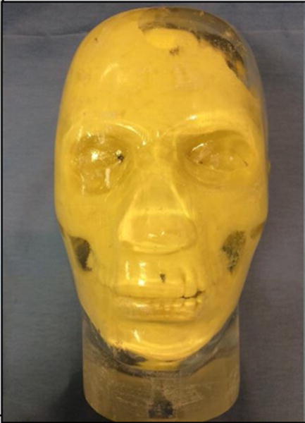
Figure 1 shows the experimental setup used for evaluating the grid-line artifact removal method. The Toshiba Infinix C-Arm system has both a standard flat panel detector and an interchangeable high-resolution CMOS detector, which is shown in its deployed position in front of the FPD. For this study, a stationary Smit-Rӧntgen x-ray grid was used with the high resolution Dexela 1207 CMOS x-ray detector (pixel size 75 μm, sensitivity area 11.5cm × 6.5cm) (Fig. 2) to image the anthropomorphic head phantoms, RS-240T, Radiology Support Devices Inc., CA (Fig. 3) and PBU-50, Kyoto Kagaku Co. Ltd., Fushimi-ku Kyoto, Japan (Fig. 4). In previous studies, we reported the results involving a simulated artery block phantom with a uniform frontal head equivalent phantom used as the scattering source to investigate the effectiveness of the method to remove the anti-scatter grid-line artifacts when a grid is used with a Flat Panel Detector (FPD) and high resolution CMOS detector.^{6, 7, 8}

Fig 1.

Experimental set-up

Fig 2.

External view of CMOS detector

Fig 3.

RS-240T

Fig 4.

PBU-50

We have also reported that the anti-scatter grid artifact correction method is equally effective when a simplified frontal head equivalent head phantom is replaced by an anthropomorphic head phantom as the scattering source⁹.

In the present study, we are demonstrating the real-time implementation of the anti-scatter grid artifact elimination method, using GPUs, on complex realistic structured images where the amount of scatter can vary across the field of view (FOV), as expected during neuro-EIGIs.

When the anthropomorphic head phantoms, PBU-50 and RS-240, were imaged using the high-resolution CMOS detector with grid placed in front it, the grid lines were prominently visible in the images. Previously it was demonstrated that removal of the grid lines by dividing the images by the flat field image obtained with grid, do not get rid of the grid artifacts completely due to presence of residual scatter (scatter which passed through the grid and reached the detector). This is an additive component, while the primary x-ray attenuation is a multiplicative factor. So the correction process first involved the removal of this additive scatter component from the input images and then dividing the scatter free image by the grid flatfield image. Since the scatter is a not uniform throughout the image, the first step of the correction is the estimation of scatter in the image.

For estimation of the residual scatter, round lead disks or markers (1 mm thick with 3 mm diameter) were used. Knowing that the lead disks block all the incident primary x-ray radiation, we placed the lead disks at different portions of the RS-240T anthropomorphic head phantom and imaged it using the high resolution CMOS detector with a grid placed in front of the detector. With the primary x-ray beam blocked, the signal registered by the detector under the lead marker position was the residual scattered radiation penetrating the grid. We placed the lead markers at 40 different locations throughout the whole field of view (FOV) of the detector and the gray scale values under all the lead marker were obtained. Knowing the gray scale (scatter) value at these 40 locations and the fact that scatter is a low spatial frequency distribution, we obtained the complete 2D scatter profile by interpolating these gray scale values between the markers, throughout the whole FOV. This scatter profile was used as the starting point for the iterative correction process. In order to reduce the time spent in iteration and to make the anti-scatter grid artifact correction fast, Graphics Processing Units (GPUs) were used.

Fig 5 shows the flowchart of the iteration process which is performed to correct the image. In one of our previous studies, we showed that the presence of anti-scatter grid lines is one of the main contributors to the standard deviation of the pixel values and as the grid-lines are removed from the image, the standard deviation of the pixel values also go down [4]. Hence, in the iteration process, our criteria was to look for the correction factors (CF) in each region which when multiplied with initial scatter estimation (S) for that region gives us the appropriate scatter amount, which when subtracted from the input image and then divided by the grid flatfield image gives us minimum value of standard deviation of gray scale values in that particular region, thus getting rid of grid artifacts.

Fig 5.

Flowchart showing iteration process for finding correct scatter profile using GPU

The CF is defined as below

$$\mathit{CF}(i)=\frac{100-(10\ast i)}{100},\mathrm{where}i(\mathrm{iteration}\mathrm{number})=0,1,2,3\dots \dots \dots \dots 9$$

The iteration steps are summarized below.

1. Scatter correction: In this step, first the CF (same to the entire image) as defined above is multiplied to the initial scatter estimation profile (S). This is then subtracted from the image to be corrected which is then divided by the grid reference image (as shown in the flow chart). This step is performed on the GPU

2. Variance (i) is calculated: In this step first the image is divided into blocks of NxN pixels (21 × 21 for this work). For each block first the variance of the grayscale values of the corrected image is calculated. If the variance of the corrected image obtained using current iteration (i) is greater than the variance obtained from the iteration (i-1), then for this particular block (or the region of the image) the minimum variance is achieved by using the correction factor as (i-1). If not then the minimum is still achieved in this iteration. This step is performed in the GPU. The operation on different blocks are performed in parallel.

3. Perform this iteration 10 times.

4. Correction factor map blurring: Once all the iterations are done a CF map consisting of individual correction factors for each region of NxN pixels of the image is generated. This correction factor map is then blurred, by blurring together MxM pixels (21× 21 pixels convolved with a kernel of 1’s in this work), to remove the discontinuity among the adjacent correction factors, which if not smoothen out will appear as a pattern on the corrected image.

5. Final scatter correction: In the last step, the blurred correction factor map of the image obtained after the iteration process is multiplied by the initial scatter profile of the image, to obtain the final residual scatter profile present in the image. This final scatter profile is subtracted from the image to be corrected, before dividing by the grid reference image, to obtain the images free from anti-scatter grid-line artifacts.

Tube parameters used for this study were 100kVp, 100mA and 12ms and these parameters, and hence the exposure, were kept the same for all acquisitions. The FOV used was 15 cm × 15 cm at the image receptor.

As an evaluation of this anti-grid scatter correction method using GPUs, we corrected the images of the PBU-50 anthropomorphic head phantom taken with the high resolution CMOS detector with grid in place. In order to correct the images of PBU-50, we did not obtain a separate scatter profile by placing lead in the beam while imaging PBU-50. Rather, we used the already estimated scatter profile obtained by placing the lead markers in the beam for RS-240T anthropomorphic head phantom, as the starting point for the iteration process.

The grid used for this study is the standard grid presently used for the Flat Panel Detector (FPD). The following Table 1 shows the relevant specifications of the grid used:

Table 1.

Grid specifications

Line rate	70 line/cm
Grid ratio	13 : 1
Absorption material	Lead, 27.5 μ
Interspace material	Fiber

The following are the set-ups used to acquire the images:

1. Table with grid (grid reference image): In this set-up, we placed the frontal head phantom (with the uniform section of the artery block inserted) on the x-ray tube. The purpose of keeping the frontal head phantom on the tube is to make sure that the x-ray beam filtration remains consistent. The grid is placed in front of the CMOS detector and the patient table is in the beam. Since, both, table and grid, are in the beam, hence this set up is named ‘Table with grid’. This set-up provides the grid reference image.

2. Object with grid: In this set-up, the frontal head phantom is removed from the tube and anthropomorphic head phantom is placed on the table. The grid is still placed in front of the CMOS detector. Since, both, object (placed on table) and grid, are both in the beam, hence this set up is named as ‘Object with grid’. This set-up provides the images of the anthropomorphic head phantom to be corrected.

3. Object without grid: In this set-up, everything remains in the same place as ‘Object with grid’, except that the grid is carefully removed from the front of the CMOS detector. Since, the object is in the beam but not the grid, this set-up is named as ‘Object without grid’. This set-up provides us images of the anthropomorphic head phantom without grid for comparison. The images obtained after anti-scatter grid corrections can be compared with ‘Object without grid’ images for qualitative and quantitative analysis.

2. RESULTS AND DISCUSSION

As expected, the anti-scatter grid correction method worked well and we were successfully able to remove the grid lines from the images of the PBU-50 head phantom with the time taken to obtain the corrected image being only 87 ms (compared to our previous CPU implementation which was approximately 12 seconds). Hence, it is established that once we have an estimated scatter profile, it can be used successfully as the starting point of iterations for different heads.

Fig. 6 shows the RS-240T anthropomorphic head phantom imaged with the FPD detector. Since the vessels in this head phantom are filled with iodine, they appear sharper in the image. Some of the important arteries like the Internal Carotid Artery (ICA), Middle Cerebral Artery (MCA), Anterior Cerebral Artery (ACA) and Petro Cavernous Artery (PCA) are visible and identified in Fig 6. The dotted region shows the portion of the RS-240T head phantom which is imaged by the CMOS detector as shown in Fig. 7.

Fig 6.

RS-240T anthropomorphic head phantom imaged with the FPD.

The selected region shows the portion of the head phantom imaged by the CMOS detector as shown in Fig 7.

Fig 7.

RS-240T phantom imaged with grid attached to CMOS detector.

Grid-lines were present in the images (and were clearly visible when we zoom into the images) when we imaged the RS-240T and PBU-50 anthropomorphic head phantoms with the high resolution CMOS detector with grids placed in front of the detector (Fig 7) (Fig 12). However, the grid-lines were successfully removed after following the earlier mentioned anti-scatter grid correction method.

Fig 12.

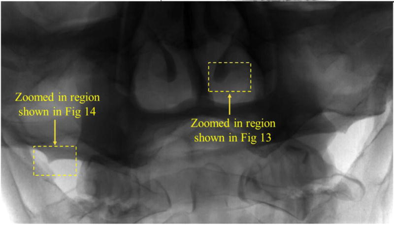
PBU-50 phantom imaged with grid attached to CMOS detector.

Fig 7 shows the RS-240T anthropomorphic head phantom imaged by the CMOS detector with the grid placed in front of the detector. Fig 8 shows the final scatter profile, obtained after the iteration process using the GPU, used to remove the grid-line artifacts from Fig 7.

Fig 8.

Final scatter distribution that was subtracted from Fig 7 to remove the residual anti-scatter grid lines (brighter indicates higher scatter).

In order to show the effectiveness of the grid-artifact correction method, we chose two different regions of Fig 6 in which the grayscale value is varying throughout the region so that the effectiveness of the method can be tested in the regions with a lot of anatomical details and features.

We equally zoomed into the two selected regions and compared the following four cases:

1. Object with grid.

2. Object with grid: Table and Grid correction – In this case, we divided the “Object with grid” image by the “Grid reference image”. No scatter is subtracted in this case.

3. Object with grid: Table, Grid and Scatter correction – In this case, we first subtracted the scatter (Fig. 8) from the “Object with grid” image, before dividing it by the “Grid reference image”.

4. Object without grid.

We also calculated the contrast and contrast–to-noise ratio (CNR) in the zoomed-in images for quantitative comparison purposes using the following equations:

$$\mathit{Contrast}(\%)=\frac{{\mathit{I}}_{\mathit{background}}-{\mathit{I}}_{\mathit{signal}}}{{\mathit{I}}_{\mathit{background}}}\times \mathbf{100},\mathit{Noise}(\%)=\frac{{\mathit{\sigma }}_{\mathit{background}}}{{\mathit{I}}_{\mathit{background}}}\times \mathbf{100},\mathit{CNR}=\frac{\mathit{Contrast}}{\mathit{Noise}}$$

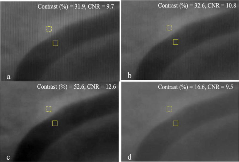
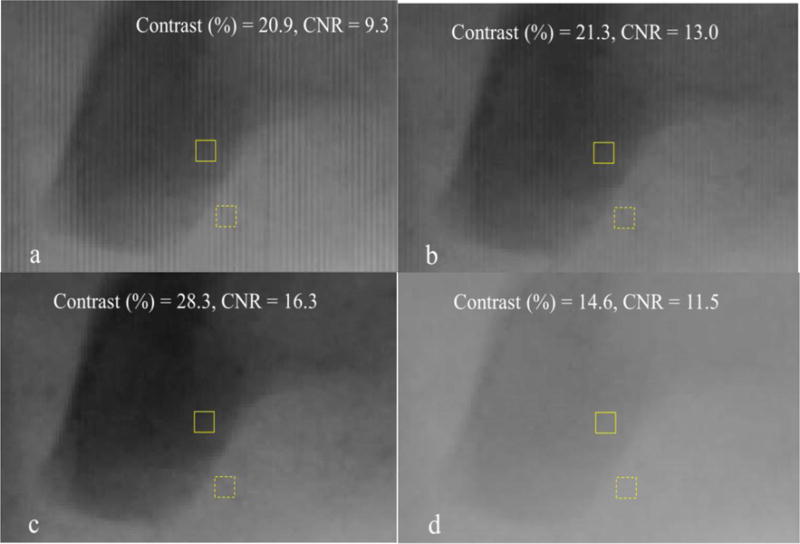
In order to calculate the contrast and CNR, we chose two regions in the image as ‘signal’ and ‘background’. A rectangular box (7 pixels × 9 pixels) was selected in small darker regions to serve as ‘signal’ and the ame size box was selected in a somewhat lighter region close by as ‘background’. The solid box and dotted box represent the signal region and the background region, respectively, in the images of Figs. 9, 10, 13 and 14. The Contrast and CNR is then calculated and compared in the same regions for all the above mentioned four cases. We observed that the improvement in contrast in all the images is quite large as compared to the respective CNR improvement. It is mainly because the exposure parameters for all the images were kept the same, irrespective of whether grid is used or not.

Fig 9.

(a) Object with grid, (b) Object with grid: Table and Grid corrected, (c) Object with grid – Table, Grid & Scatter corrected (d) Object without grid

Fig 10.

(a) Object with grid, (b) Object with grid: Table and Grid corrected, (c) Object with grid – Table, Grid & Scatter corrected (d) Object without grid

Fig 13.

(a) Object with grid, (b) Object with grid: Table and Grid corrected, (c) Object with grid – Table, Grid & Scatter corrected (d) Object without grid

Fig 14.

(a) Object with grid, (b) Object with grid: Table and Grid corrected, (c) Object with grid – Table, Grid & Scatter corrected (d) Object without grid

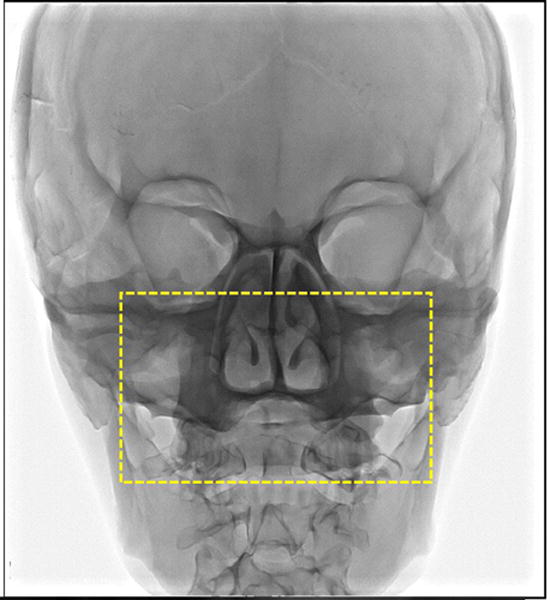
Fig 11 shows the PBU-50 anthropomorphic head phantom images taken with the FPD detector. This head phantom has skull embedded into a soft tissue substitute. The dotted region shows the portion of the PBU-50 head phantom imaged using the high resolution CMOS detector.

Fig 11.

PBU-50 anthropomorphic head phantom imaged with the FPD.

The selected region shows the portion of the head phantom imaged by the CMOS detector as shown in Fig 12.

3. CONCLUSIONS

We demonstrated that the images of the head phantoms taken with a grid using a high resolution CMOS detector can be corrected in real time using GPUs by iteratively determining the scatter value providing a minimum pixel variance in all the regions across the field of view in the image when the grid-correction method (i.e. division by the reference uniform field grid image) was used. We divided the full field of view into small regions and iterated to minimize the artifact in each region in parallel with the GPU capability. Thus, with the use of the computational tools, we are able to demonstrate how to correct the images for anti-scatter grid artifacts immediately after acquisition, during dynamic sequences such as used in neuroendovascular image-guided interventional procedures.

References

- 1.Neitzel U. Grids or air gaps for scatter reduction in digital radiography: a model calculation. Medical physics. 1992;19(2):475–481. doi: 10.1118/1.596836. http://www.ncbi.nlm.nih.gov/pubmed/1584148. [DOI] [PubMed] [Google Scholar]
- 2.Barnes GT. Contrast and scatter in x-ray imaging. Radiographics : a review publication of the Radiological Society of North America Inc. 1991;11(2):307–323. doi: 10.1148/radiographics.11.2.2028065. http://www.ncbi.nlm.nih.gov/pubmed/2028065. [DOI] [PubMed] [Google Scholar]
- 3.Bednarek DR, Rudin S, Wong R. Artifacts produced by moving grids. Radiology. 1983;147(1):255–258. doi: 10.1148/radiology.147.1.6828740. http://www.ncbi.nlm.nih.gov/pubmed/6828740. [DOI] [PubMed] [Google Scholar]
- 4.Rudin S, Bednarek DR, Hoffman KR. Endovascular image-guided interventions (EIGIs) Med Phys. 2008;35(1):301–309. doi: 10.1118/1.2821702. http://www.pubmedcentral.gov/articlerender.fcgi?artid=2669303. [DOI] [PMC free article] [PubMed] [Google Scholar]
- 5.Gauntt DM, Barnes GT. Grid line artifact formation: A comprehensive theory. Medical physics. 2006;33(6):1668–1677. doi: 10.1118/1.2184444. http://www.ncbi.nlm.nih.gov/pubmed/16872074. [DOI] [PubMed] [Google Scholar]
- 6.Singh V, Jain A, Bednarek DR, Rudin S. Limitations of anti-scatter grids when used with high resolution image detectors. Proceedings SPIE (Medical Imaging 2014) doi: 10.1117/12.2043063. http://www.ncbi.nlm.nih.gov/pmc/articles/PMC4189125/ [DOI] [PMC free article] [PubMed]
- 7.Rana R, Singh V, Jain A, Bednarek DR, Rudin S. Anti-scatter grid artifact elimination for high resolution x-ray imaging CMOS detectors. Proceedings SPIE (Medical Imaging 2015) doi: 10.1117/12.2081430. https://www.ncbi.nlm.nih.gov/pmc/articles/PMC4749028/ [DOI] [PMC free article] [PubMed]
- 8.Rana R, Bednarek DR, Rudin S. Grid-line artifact minimization for high resolution detectors using iterative residual scatter corrections. Medical Physics. 2015;42(6):3695. http://scitation.aip.org/content/aapm/journal/medphys/42/6/10.1118/1.4926090. [Google Scholar]
- 9.Rana R, Jain A, Shankar A, Bednarek DR, Rudin S. Scatter estimation and removal of anti-scatter grid-line artifacts from anthropomorphic head phantoms images taken with a high resolution image detector. Proceedings SPIE (Medical Imaging 2016) doi: 10.1117/12.2216833. http://spie.org/Publications/Proceedings/Paper/10.1117/12.2216833. [DOI] [PMC free article] [PubMed]