

Abstract
Health impact assessments for fine particulate matter (PM2.5) often rely on simulated concentrations generated from air quality models. However, at the global level, these models often run at coarse resolutions, resulting in underestimates of peak concentrations in populated areas. This study aims to quantitatively examine the influence of model resolution on the estimates of mortality attributable to PM2.5 and its species in the USA. We use GEOS-Chem, a global 3-D model of atmospheric composition, to simulate the 2008 annual average concentrations of PM2.5 and its six species over North America. The model was run at a fine resolution of 0.5 × 0.66° and a coarse resolution of 2 × 2.5°, and mortality was calculated using output at the two resolutions. Using the fine-modeled concentrations, we estimate that 142,000 PM2.5-related deaths occurred in the USA in 2008, and the coarse resolution produces a national mortality estimate that is 8 % lower than the fine-model estimate. Our spatial analysis of mortality shows that coarse resolutions tend to substantially underestimate mortality in large urban centers. We also re-grid the fine-modeled concentrations to several coarser resolutions and repeat mortality calculation at these resolutions. We found that model resolution tends to have the greatest influence on mortality estimates associated with primary species and the least impact on dust-related mortality. Our findings provide evidence of possible biases in quantitative PM2.5 health impact assessments in applications of global atmospheric models at coarse spatial resolutions.
Keywords: Health impact assessment, PM2.5, Species, Grid resolution, Premature mortality
Introduction
Epidemiological studies have linked exposure to ambient fine particulate matter (PM2.5) with a wide spectrum of adverse health outcomes, from acute respiratory symptoms to premature deaths. These studies have demonstrated significant associations between both short-term and long-term mortality and exposure to PM2.5 (Beelen et al. 2008; Dockery et al. 1993; Filleul et al. 2005; Krewski et al. 2009; Laden et al. 2006; Ostro 2004; Pope et al. 2002).
An air quality health impact assessment is an integrated procedure that synthesizes information about air pollution exposures, health effects, and population vulnerability (Kheirbek et al. 2013). This approach has been applied in estimating the burden of disease attributed to air pollution at the national and global levels (Anenberg et al. 2010; Cohen et al. 2005; Fann et al. 2013; Li et al. 2010) and potential public health benefits associated with air quality regulations (Li and Crawford-Brown 2011; Wang and Mauzerall 2006).
Health impact assessments commonly rely on pollutant concentrations modeled with air quality models. Models are very useful tools in this setting because they enable examination of alternative scenarios related to factors such as air pollution emissions, climate, and population growth. In addition, since observational data for air pollutants are only available at limited monitoring locations, model-simulated concentrations have advantages in capturing health impacts that are more spatially and temporally complete than monitoring data. However, grid cell resolution can be limited by computational power, particularly on a larger scale such as global atmospheric models. These models often run at resolutions of roughly 100–400 km (Anenberg et al. 2010, 2012; Bey et al. 2001; West et al. 2006). For PM2.5, many of the species that make up its total mass concentration are formed in the atmosphere from chemical reactions between precursor species (Thompson et al. 2014). Strong spatial concentration gradients of emissions can influence chemical production, leading to errors at too coarse resolution due to spatial averaging of emissions (Thompson et al. 2014). As a result, coarse resolution may suppress high urban PM2.5 concentrations. This in turn can lead to biased health impact estimates. Coarse models do not resolve important relationships between gradients in population and gradients in air pollution. When these gradients are positively correlated, as for black carbon (BC) and other primary anthropogenic PM species, a coarse model will tend to underestimate health impacts. When they are anti-correlated, as for natural dust, a coarse model will tend to overestimate health impacts.
While studies have been conducted to investigate the effect of resolution on predicted PM2.5 concentrations (Arunachalam et al. 2011; De Meij et al. 2007; Mensink et al. 2008), the influence of grid resolution on health impact assessment for PM2.5 is not yet well understood. Given the importance of grid resolution on both predicted concentrations and population exposure in a health impact assessment for PM2.5, some recent studies investigated how estimates of health impacts at coarser resolution differ from those at fine resolution (Punger and West 2013; Thompson et al. 2014). However, these studies have reported conflicting results: one found that coarse grid resolutions produce national mortality estimates in the USA that are substantially biased low (Punger and West 2013), whereas the other reported that health impacts associated with changes in PM2.5 concentrations were not sensitive to model resolution (Thompson et al. 2014). Furthermore, these studies relied on urban- and regional-scale model simulations, and studies have not been conducted using simulations from global atmospheric models. In addition, most studies focus on total PM2.5 mass. Since coarse model resolution is thought to affect primary particulates much more strongly than secondary particulate matter (EPA 2007; Punger and West 2013), the effects of resolution on different PM2.5 species warrant further investigation.
This study quantitatively examines the influence of model resolution on estimates of premature mortality attributable to PM2.5 and its chemical components in the USA. We use a global atmospheric model to simulate annual average concentrations of six PM2.5 species: black carbon (BC), ammonium (NH4), nitrate (NIT), sulfate (SO4), organic carbon (OC), and dust (DST) at two spatial resolutions. We also re-grid the fine-scale estimate to coarser scales. Overall, our main study purpose is to help understand possible biases in health impact assessment results across a range of PM species due to coarse grid resolutions of global atmospheric models.
The remainder of the paper is organized as follows: the “Methodology” section describes details of modeling annual average concentrations of air pollutants and the methods used to quantify mortality associated with pollutant exposure in the USA. The “Results and discussions” section presents our mortality estimates at various modeled and re-gridded resolutions. For each PM2.5 species, we quantify how mortality estimates differ from the fine-model resolution to the coarse-model resolution, and from the fine-model resolution to the re-scaled coarser resolutions. We compare the difference in mortality estimates at the national level and county level. The “Discussion and conclusions” section summarizes the conclusions of this study and proposes issues to be further investigated in future work.
Methodology
Overview of the method
We evaluate the effect of model resolution on health impact assessment by calculating annual mortality attributable to total PM2.5 and six of its principal component species in the continental USA using modeled and scaled pollutant concentrations. We then compare the mortality estimates based on various modeled or scaled model output to explore the bias resulted from coarse resolution.
The health impacts of PM2.5 and its species are calculated based on the following components: simulated air concentrations, the size of the affected population, baseline mortality rates, and concentration–response functions abstracted from epidemiologic literature. These factors are combined in an integrated procedure using a health impact function. A log-linear health impact function to quantify the excess mortality attributed to air pollution is (Anenberg et al. 2012; Li et al. 2010)
| (1) |
where
| ∆y | Excess mortality attributable to pollutant exposures |
| β | Concentration–response coefficient from epidemiological studies (increase in mortality per unit increase in pollutant concentration) |
| ∆x | Change in air quality, taken here as the modeled pollutant concentrations |
| y0 | Baseline mortality rates |
| Pop | The affected population, i.e., the number of people exposed to PM2.5 pollution |
Here, we use BenMAP (Environmental Benefits Mapping and Analysis Program, version 4.0.67, Abt Associates 2013) to calculate the health impacts of exposure to BC. In the following sections, we first describe the GEOS-Chem air quality model used to simulate annual average PM2.5 concentrations across the continental USA. We then discuss how we select the concentration-response coefficient (β) used to estimate mortality due to PM2.5 and its species and how we characterize the affected population (Pop) and the baseline incidence rates (y0) in Eq. (1). We also discuss the approach we use to estimate mortality associated with individual species.
Modeling annual average pollutant concentrations
We use GEOS-Chem (www.geos-chem.org) (Bey et al. 2001), a global 3-D model of atmospheric composition, to simulate annual average concentrations of the six PM2.5 species over North America in 2008. GEOS-Chem is driven by assimilated meteorological observations from the Goddard Earth Observing System (GEOS) of the NASA Global Modeling Assimilation Office. Global simulations are performed at the 4° latitude × 5° longitude degree resolution, with a 6-month spin-up beginning in July 2007, through the end of 2008. Simulated 3-hourly concentrations from this global calculation are used as the boundary conditions to drive higher-resolution nested simulations over North America at the 0.5° latitude by 0.667° longitude resolution (Chen et al. 2009; Wang et al. 2004). We also computed a global-scale simulation at the 2° latitude × 2.5° longitude resolution. In addition, we re-gridded the modeled concentrations from the 0.5° × 0.667° simulation to several coarser resolutions through simple averaging, including 1° latitude × 1.25° longitude, 2° latitude × 2.5° longitude, and 4° latitude × 5° longitude. The standard BenMAP configuration requires the national 12-km Community Multiscale Air Quality (CMAQ) model grid to evaluate air quality model output. Therefore, we convert all model results to the national 12 × 12 km2 grid using a two-step process. GEOS-Chem binary punch output is first converted to Climate Forecasting compliant NetCDF with PseudoNetCDF (pseudonetcdf.googlecode.com) and then re-gridded using a first-order conservative method as implemented in the Climate Data Operators (code.zmaw.de/projects/cdo).
The GEOS-Chem aerosol simulation includes treatment of the ammonium–nitrate–sulfate–water particulate equilibrium (Fountoukis and Nenes 2007; Park et al. 2004), elemental and organic carbonaceous aerosol (Park et al. 2003), dust (Duncan Fairlie et al. 2007), and sea salt (Alexander et al. 2005; Jaeglé et al. 2011). In this study, we did not consider secondary organic aerosol, which likely constitutes a significant fraction of PM2.5 concentrations (Jimenez et al. 2009), as we focus more on species around which current air quality policies are designed (i.e., primary carbonaceous aerosol and the secondary inorganic species ammonium sulfate and ammonium nitrate). Aerosol dry deposition is calculated following the resistance-in-series scheme of Wesely (1989); wet removal owing to large-scale precipitation and convective scavenging follows Liu et al. (2001).
Emissions of aerosols and aerosol precursors come from several global and regional inventories. Annual emissions from biofuel and fossil fuel are from Bond et al. (2007), replaced by the inventory of Cooke et al. (1999) over North America, with monthly scaling factors applied from Park et al. (2003). Biomass burning emissions are taken from the Global Fire Emissions Database (Giglio et al. 2010; van der Werf et al. 2010). Anthropogenic emissions of NOx and SO2 are from the global 2000 inventory of EDGAR 3.2 (Olivier et al. 2005) with annual scaling factors for 2005 from van Donkelaar et al. (2008). Emissions of NH3 are described in Park et al. (2004). Emissions of SO2 and NOx in the USA are overwritten with values from the US National Emission Inventory (NEI) for 2005. Emissions of SO2, NOx, and NH3 are also overwritten by national inventories in Canada (CAC), Mexico (BRAVO), Europe (EMEP), and East Asia (Streets et al. 2006).
Simulated values of PM2.5 and component species in the USA have been extensively compared to measurements from in situ monitoring networks (Heald et al. 2012; Henze et al. 2009; Liao et al. 2007; Mao et al. 2013; van Donkelaar et al. 2010; Walker et al. 2012; Zhang et al. 2012, 2013; Zhu et al. 2013), aircraft campaigns (van Donkelaar et al. 2008; Dunlea et al. 2009; Fisher et al. 2011; Heald et al. 2011), and remote sensing observations (Generoso et al. 2008; Heald et al. 2010; Johnson et al. 2012; Luan and Jaeglé 2013; van Donkelaar et al. 2010). While the model generally well represents the overall magnitude and relative speciation of primary aerosol and secondary inorganic aerosol (Philip et al. 2014), there is a persistent overestimate of aerosol nitrate in the eastern USA (Heald et al. 2012).
Health impact assessment
Cohort studies on the associations between PM2.5 exposure and mortality have been used to estimate PM2.5-related long-term mortality in health impact assessment. Two prospective cohort studies have been conducted in the USA, often referred to as the Harvard Six-Cities (H6C) study (Dockery et al. 1993; Laden et al. 2006) and the American Cancer Society (ACS) study (Krewski et al. 2009; Pope et al. 1995, 2002). These studies have found rather consistent relationships between PM2.5 exposure and premature death across various locations in the USA. More recently, a study has developed an integrated exposure-response function (Burnett et al. 2014), which was used in the Global Burden of Diseases, Injuries, and Risk Factors Study 2010 (Lim et al. 2013).
For this study, we select the concentration-response coefficient for all-cause mortality from the recent Krewski et al. (2009) extended analysis of the ACS study, which includes a large cohort of 500,000 adults over 116 US cities. The mortality risk estimates from the ACS study have been used to assess the health burden associated with exposure to ambient PM2.5 in the USA and globally (Anenberg et al. 2010; Fann et al. 2012; Punger and West 2013). Using a 1999–2000 random-effects Cox model adjusted for 7 ecological and 44 individual covariates, Krewski et al. (2009) predicted a risk ratio of 1.06 (95 % confidence interval, CI, 1.04–1.08) for a 10-μg/m3 increase in PM2.5 concentration for all-cause mortality. This risk ratio was converted to a concentration–response coefficient value of 0.005827 used in this study (a normal distribution with a standard deviation of 0.000963). Although some studies have suggested that certain species of PM2.5, such as black carbon, may pose a greater mortality risk on human health than other components (Janssen et al. 2011; Smith et al. 2010), current evidence is still insufficient to differentiate the health effects of the various constituents of PM2.5 (EPA. 2012). Based on this, we do not differentiate the concentration–response functions for various species of PM2.5 in this study.
Earlier epidemiological studies on health effects of particles found little evidence of a threshold level for an exposure–response relation between PM and health effects (Daniels et al. 2000; Krewski et al. 2009; Pope 2000; Schwartz et al. 2002). In this study, we estimate premature mortality due to PM2.5 and its species without applying a threshold level below which pollutants are assumed to have no health effect.
We use the 2008 population and baseline mortality rates data that have been built into BenMAP. BenMAP uses Census block data to calculate the population level in the population grid cells (Abt Associates 2013). We use the population at the national 12-km grid resolution, and the modeled pollutant concentrations are matched with the population in each 12-km grid cell. Also, population data in BenMAP are stratified by age. We select population aged over 30 in order to be consistent with the Krewski et al. (2009) study from which we draw the risk estimate. To estimate mortality rates, BenMAP uses individual-level mortality data from 2004 to 2006 for the whole USA from the Centers for Disease Control (CDC) and National Center for Health Statistics (NCHS) (Abt Associates 2013).
We calculate mortality associated with individual PM2.5 species by directly applying the simulated annual average concentrations of each species. Another approach is to calculate mortality for the total PM2.5 concentration relative to the total PM2.5 minus one species, as was used in the study by Punger and West (2013). The main difference in the two methods lies in the fact that the approach of removing a species from the air would suggest how responsive total mortality might be to an intervention strategy focused on a specific particle type, whereas our approach directly refers to the attributable fractions of PM2.5 mortality associated with different species. However, since the concentration-response curve is nearly linear within the range of PM2.5 concentrations we consider (0–22 μg/m3), we expect the results produced from these two approaches will not differ considerably. In order to verify this assumption, we conducted a sensitivity analysis by calculating the national mortality attributable to each PM2.5 species at the modeled 0.5 × 0.66° resolution using the Punger and West approach, and then compared the mortality estimates produced from the two approaches. The results indicate that our approach produces mortality estimates for the six species that are approximately 5–7 % higher than those based on the Punger and West approach. The detailed results of this analysis are presented in Table 4 in the Appendix.
Using simulated pollutant concentrations, the selected concentration-response coefficient for all-cause mortality, and the built-in population and baseline mortality rates in BenMAP, we calculated the number of excess deaths in the USA in 2008 related to total PM2.5 and its species. We repeat the calculation using the concentrations at the two model resolutions and at the three regridded resolutions. In estimating the 95 % CI of national mortality estimates, the only source of uncertainty that is taken into account is the uncertainty in the value of the concentration-response coefficient (β, with a mean value of 0.005827). The uncertainty analysis was conducted in BenMAP using Monte Carlo simulations with a sample size of 5000. In addition to the national mortality estimates, we also calculated mortality by county to investigate how the influence of model resolution on mortality estimates may differ spatially.
Results and discussions
Pollutant concentrations at various modeled and re-gridded resolutions
Panels a and b of Fig. 1 show the GEOS-Chem modeled annual average PM2.5 concentrations in 2008 at the fine (0.5 × 0.66°) and coarse (2 × 2.5°) resolution, respectively. The maximum simulated PM2.5 value in the continental USA is 21 and 17 μg/m3 at the fine and coarse resolution, respectively. The mean PM2.5 values are both approximately 6 μg/m3 at the fine and coarse resolutions. In general, the highest PM2.5 values occur in the eastern USA. Figure 8 in the Appendix shows the modeled annual average concentrations of the six species in 2008 at the fine and coarse resolutions. For BC, NH4, and NIT, the highest values are located in the northeastern USA. For SO4 and OC, the highest values occur in the eastern USA. For DST, these values occur in the southwest border area.
Fig. 1.
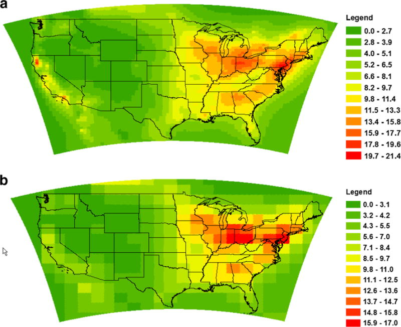
Modeled annual average PM2.5 concentrations in 2008 using GEOS-Chem output at a fine (0.5 × 0.66°) resolution and b coarse (2 × 2.5°) resolution (unit, μg/m3)
Table 1 presents the mean and maximum values for concentrations of PM2.5 and its six species at various modeled and re-gridded resolutions. For all the species and total PM2.5, the mean concentrations at various resolutions are similar. On the other hand, the maximum simulated concentrations decrease when going from the fine-model resolution (0.5 × 0.66°) to the coarse resolution (2 × 2.5°). For total PM2.5, the maximum concentration decreases 21 %. For different species of PM2.5, the percentage change in maximum concentration from the fine resolution to the coarse resolution varies. The percentage change in the maximum value for organic carbon (61 %) is the greatest, followed by black carbon (31 %), indicating that coarse-model resolutions are likely to cause peak values of primary particulates (mainly BC and OC) to be underestimated, consistent with the findings of Punger and West (2013). For regridded output, the maximum values also decrease as the resolution becomes coarse. Interestingly, the results at 2 × 2.5° agree rather closely for both the modeled and re-gridded data, suggesting that most of the bias comes from simple spatial averaging.
Table 1.
Mean and maximum simulated concentrations of PM2.5 and its six components at various modeled (0.5 × 0.66 and 2 × 2.5°) and re-gridded (1 × 1.25, 2 × 2.5, and 4 × 5°) resolutions over the continental USA (year, 2008; unit, μg/m3)
| Species | Modeled output
|
Re-gridded output
|
|||||||||
|---|---|---|---|---|---|---|---|---|---|---|---|
| 0.5 × 0.66°
|
2 × 2.5°
|
% change of the max value | 1 × 1.25°
|
2 × 2.5°
|
4 × 5°
|
||||||
| Mean | Max | Mean | Max | Mean | Max | Mean | Max | Mean | Max | ||
| BC | 0.32 | 3.2 | 0.32 | 2.2 | −31 % | 0.32 | 2.8 | 0.32 | 2.3 | 0.32 | 1.5 |
| NH4 | 0.8 | 3.2 | 0.8 | 2.8 | −13 % | 0.8 | 2.8 | 0.8 | 2.6 | 0.8 | 2.3 |
| NIT | 1.1 | 6.6 | 1.1 | 5.9 | −11 % | 1.1 | 5.8 | 1.1 | 5.4 | 1.1 | 5.0 |
| SO4 | 1.5 | 4.5 | 1.3 | 3.2 | −29 % | 1.5 | 3.9 | 1.5 | 3.7 | 1.5 | 3.5 |
| OC | 1.3 | 14.6 | 1.3 | 5.7 | −61 % | 1.3 | 7.9 | 1.3 | 5.7 | 1.3 | 4.0 |
| DST | 0.69 | 6.1 | 0.96 | 5.8 | −5 % | 0.69 | 4.6 | 0.69 | 3.0 | 0.69 | 2.4 |
| PM2.5 | 5.7 | 21.4 | 5.8 | 17 | −21 % | 5.7 | 18.7 | 5.7 | 17.3 | 5.7 | 14.5 |
Premature mortality due to PM2.5 exposure based on model output
As shown in Table 2, using the GEOS-Chem modeled results at the fine resolution, we estimate that approximately 142,000 (95 % CI, 97,500–186,400) all-cause deaths occurred in the USA in 2008 due to ambient PM2.5 exposure. The coarse-model results produce an estimate of all-cause mortality that is 8 % lower than the estimate based on the fine-model results (approximately 130,000 deaths totally, 95 % CI, 89,000–171, 000). Figure 2 shows the annual PM2.5-related mortality at the 12-km resolution calculated using the fine (0.5 × 0.66°) resolution model results. In general, the greatest densities of deaths occur in populated areas in the eastern USA and west coast. Our estimates of national PM2.5 mortality are similar to a recent estimate of national mortality associated with exposure to ambient PM2.5 (Fann et al. 2012), but greater than those of Punger and West (2013). Using the photochemical Community Multiscale Air Quality (CMAQ) model results at a 12-km grid resolution in conjunction with ambient monitored data, and the same all-cause mortality risk estimate from Krewski et al. (2009), Fann et al. (2012) estimated 130,000 (95 % CI, 51,000–200,000) PM2.5-related deaths to result from 2005 air quality levels, relative to regional PM2.5 background concentrations (ranging from 0.62 to 1.72 μg/m3, depending on the region). Using the same CMAQ model results at a 12-km resolution in 2005, Punger and West (2013) report a national mortality estimate of 66,000 (95 % CI, 39,300–84,500) due to PM2.5 exposure, relative to the low-concentration exposure threshold of 5.8 μg/m3 (Krewski et al. 2009). Since we apply the same concentration–response function from Krewski et al. (2009), differences in national mortality estimates between our study and these other studies are due in part to the selection of threshold (we apply no threshold in our calculation). If a 5.8-μg/m3 threshold is applied, our estimates of PM2.5-related mortality would be 70,000 (95 % CI, 48,000–92,500) at the 0.5 × 0.66° model resolution and 58,000 (95 % CI, 39,500–76,200) at the 2 × 2.5° model resolution. These estimates are close to the Punger and West (2013) estimates.
Table 2.
National mortality in the USA in 2008 attributed to PM2.5 exposure estimated using various modeled and re-gridded resolutions
| Species | Modeled output
|
Re-gridded output
|
||||||||
|---|---|---|---|---|---|---|---|---|---|---|
| 0.5×0.66°
|
2×2.5°
|
1×1.25°
|
2×2.5°
|
4×5°
|
||||||
| Mean | 95 % CI | Mean | 95 % CI | Mean | 95 % CI | Mean | 95 % CI | Mean | 95 % CI | |
| BC | 13,280 | 8993−17,557 | 11,211 | 7590−14,827 | 12,305 | 8331−16,271 | 11,320 | 7664−14,970 | 9082 | 6147−12,014 |
| NH4 | 20,464 | 13,862−27,048 | 18,471 | 12,511−24,417 | 19,560 | 13,250−25,856 | 19,343 | 13,102−25,568 | 17,782 | 12,043−23,507 |
| NIT | 32,683 | 22,175−43,140 | 30,535 | 20,717−40,305 | 30,163 | 20,461−39,820 | 29,659 | 20,119−39,156 | 26,548 | 18,005−35,055 |
| SO4 | 32,539 | 22,065−42,972 | 26,795 | 18,161−35,400 | 32,348 | 21,935−42,720 | 32,252 | 21,870−42,593 | 30,761 | 20,856−40,629 |
| OC | 40,144 | 27,246−52,974 | 36,540 | 24,790−48,235 | 38,459 | 26,098−50,760 | 36,593 | 24,827−48,304 | 32,382 | 21,960−42,761 |
| DST | 7372 | 4988−9753 | 10,177 | 6888−13,461 | 7374 | 4990−9756 | 7411 | 5015−9804 | 7469 | 5054−9880 |
| PM2.5 total | 142,342 | 97,463−186,431 | 130,249 | 89,089−170,746 | 136,433 | 93,362−178,782 | 132,955 | 90,963−174,256 | 121,050 | 82,725−158,804 |
Fig. 2.
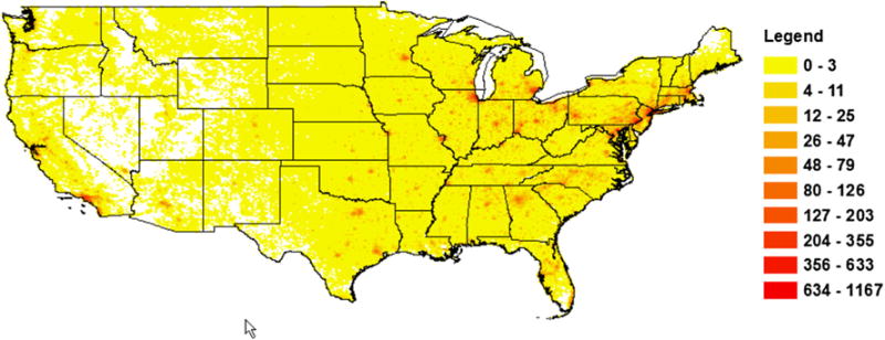
Annual all-cause mortality at 12-km resolution due to total PM2.5 in 2008 estimated using GEOS-Chem output at the fine (0.5 × 0.66°) resolution (deaths per year)
Figure 3 compares the mortality estimates attributed to each PM2.5 species based on model estimates at the fine (0.5 × 0.66°) resolution versus the coarse (2 × 2.5°) resolution. When moving from fine to coarse resolution, mortality estimates due to all species decrease except for dust. Among the five species, mortality estimates due to SO4 decrease the most (18 %), followed by BC (16 %). For dust, the mortality estimate at the coarse resolution is 38 % higher than that at the fine resolution.
Fig. 3.
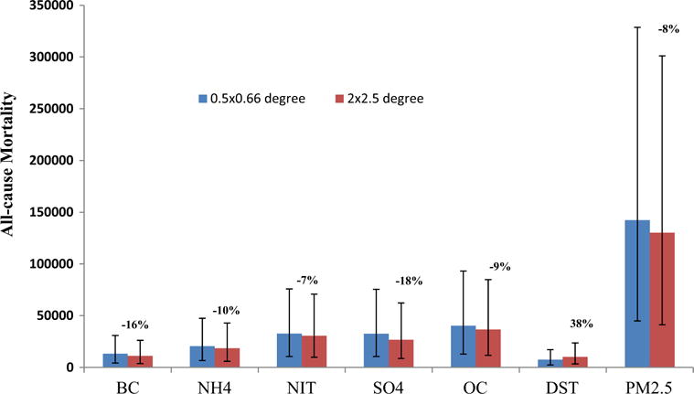
Total mortality in the USA in 2008 attributed to each species, fine versus coarse resolution (Error bars show the 95 % CI; percent values shown are percentage changes relative to the estimates at the fine resolution)
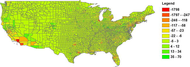
To examine the influence of model resolution on aggregated mortality estimates, we calculated the population-normalized difference in estimated mortality by county between the fine-model resolution and the coarse resolution (Fig. 4; also refer to Fig. 10 in the Appendix for the map that shows the difference in mortality without population normalization). These results show that the coarse resolution tends to significantly underestimate the county-level mortality estimates in large urban centers (counties shown in red in Fig. 4).
Fig. 4.
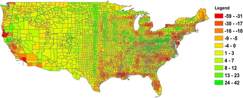
The population-normalized difference in estimated mortality by county attributed to total PM2.5 between the fine-model resolution (0.5 × 0.66°) and the coarse resolution (2 × 2.5°) (calculated as the coarse resolution estimate minus the fine resolution estimate, divided by population; shown as difference in mortality per 100,000 people)
In order to further investigate the influence of model resolution on aggregated mortality attributed to different PM2.5 species, we also compared the maximum death values at the county level based on the two model resolutions. Table 3 compares the difference in the maximum mortality estimates in a county between estimates calculated using model output at the fine and coarse resolutions. For all five species except dust, the maximum mortality estimates decrease from the fine resolution to the coarse resolution. The maximum values for BC and OC decrease much more significantly compared to the values for NH4, NIT, and SO4. For total PM2.5 mass, the maximum value, located in Los Angeles County, CA, is 46 % less at the coarse resolution compared to the fine resolution. These results indicate that coarse-model resolutions are likely to cause the greatest density of PM2.5-related deaths to be underestimated, particularly deaths due to primary particulates (mainly BC and OC). For dust, the maximum county-level estimate at the fine resolution, located in Maricopa County, AZ, decreases slightly by 3 % at the coarse resolution. However, the mortality estimate in Los Angeles, CA, increases 71 % from the fine to the coarse resolution. The decrease in the estimated mortality for most species can be explained by the decrease in peak PM2.5 concentrations due to the use of coarser resolution, as these peaks typically occur in populated urban centers. For dust, however, the change in the estimated mortality shows an opposite sign from the other species. This can be explained by the fact that the sources of dust are in remote areas and hence dust concentrations are largely uncorrelated with population (as shown in Fig. in the Appendix).
Table 3.
Maximum mortality estimate at the county level attributed to PM2.5 and its six species, calculated using modeled concentrations at 0.5 × 0.66° and 2 × 2.5° over the continental USA
| Species | Maximum morality estimate at the county level
|
County | % change of the maximum value | |
|---|---|---|---|---|
| 0.5×0.66° | 2×2.5° | |||
| BC | 812 | 382 | Los Angeles, CA | −53 % |
| NH4 | 492 | 460 | Cook, IL | −7% |
| NIT | 1039 | 932 | Cook, IL | −10 % |
| SO4 | 533 | 516 | Cook, IL | −3% |
| OC | 1425 | 787 | Los Angeles, CA | −45 % |
| DST | 349 (max value) | 339 | Maricopa, AZ | −3% |
| 289 | 494 | Los Angeles, CA | 71 % | |
| PM2.5 | 3935 | 2137 | Los Angeles, CA | −46 % |
PM2.5-related premature mortality estimates based on re-gridded concentrations
Comparing the coarse re-gridded results with the finest model results
For total PM2.5, increasing grid size decreases the estimated mortality (Fig. 5; also refer to Fig. 11 in the Appendix for the original estimates of national all-cause mortality due to PM2.5 species at various grid resolutions). At the 1 × 1.25° resolution, total estimated PM2.5-related mortality is 4 % lower than the fine resolution (0.5 × 0.66°) estimate; the 2 × 2.5° and 4 × 5° resolutions produce mortality estimates that are 7 and 15 % lower than the estimate driven with the fine resolution, respectively. The decrease in total mortality estimates can be explained by the decrease in peak PM2.5 concentrations, which typically occur in populated regions, due to dilution into a coarser grid cell (Punger and West 2013). As a result of the dilution of peak concentrations in populated areas, coarse resolutions tend to underestimate the high density of deaths occurring in these areas.
Fig. 5.
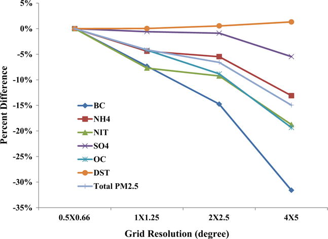
Percent difference in estimates of national all-cause mortality due to PM2.5 species between the re-gridded resolution and the fine-model resolution, calculated as (re-gridded, coarse results-fine-model results)/fine-model results
For all the five species except dust, the estimated mortality decreases as the resolution becomes coarser. At the coarsest 4 × 5° resolution, mortality estimate decreases the most for BC (a 32 % decrease relative to the finest model result), followed by OC (a 19 % decrease relative to the finest model result). In general, coarse resolution tends to have the greatest influence on the estimates of national mortality associated with exposure to primary species (mainly BC, and OC contains both primary and secondary particles). Our findings of the effect of grid resolution on primary and secondary species of PM2.5 are consistent with those of Punger and West (2013), who reported that coarse resolution has the greatest percentage effect on estimates of mortality driven with primary species. For dust, this is only a small change (a 1 % increase) in mortality estimate at the 4 × 5° resolution relative to the finest resolution.
As shown in Fig. 6, at 1 × 1.25 re-gridded resolution, mortalities in counties where large cities are located (mostly in the eastern USA and on the west coast) are underpredicted, whereas the biases are small in most other counties. The error is the largest in Los Angeles County in California. At 2 × 2.5 resolution, the error (underprediction) becomes even larger in Los Angeles County, whereas the errors in a few counties surrounding Los Angeles County become smaller compared to the 1 × 1.25 resolution. On the other hand, comparing to the 1 × 1.25 resolution, most counties slightly over-predict mortality at 2 × 2.5 resolution. Finally, at 4 × 5 resolution, the error in Los Angeles County is the largest whereas mortality is over-predicted in most counties in the USA to a larger extent.
Fig. 6.
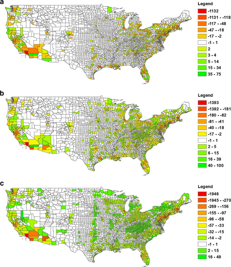
Difference in the estimated all-cause deaths by county attributable to PM2.5 exposure in 2008 due to re-gridded coarse resolution, calculated as a the 1 × 1.25 estimates minus the 0.5 × 0.66 estimates; b the 2 × 2.5 estimates minus the 0.5 × 0.66 estimates; and c the 4 × 5 estimates minus the 0.5 × 0.66 estimates (counties with the difference falling into the range of [−1, 1] are shown in white color)
Comparing the modeled and re-gridded results both at the 2 × 2.5° resolution
We also compared the model and re-gridded results at the same 2 × 2.5° resolution. As shown in Table 2, for national mortality estimates, modeled and re-gridded concentrations at the 2 × 2.5° resolution produce similar results for BC, NH4, NIT, and OC. For SO4, however, the mortality estimate based on the re-gridded concentrations is 20 % greater than the estimate based on the modeled concentrations, and for dust, the re-gridded results produce a national mortality estimate that is 27 % less. Overall, the total PM2.5-related mortality predicted from the re-gridded output is 2 % higher than that predicted from the modeled 2 × 2.5° resolution output. Although it seems that the re-gridded concentrations at the 2 × 2.5° resolution produce a national PM2.5-related mortality estimate that is very close to the estimate based on model output at the same resolution, for different PM2.5 species, the differences between the two estimates vary.
Figure 7 shows the difference in mortality due to PM2.5 at the county level between the modeled and re-gridded 2 × 2.5° resolution. It indicates that in the eastern USA and the west coast, the re-gridded output tends to overestimate PM2.5-related mortality whereas in the western USA (except for the west coast), the re-gridded results are likely to underestimate PM2.5 mortality.
Fig. 7.
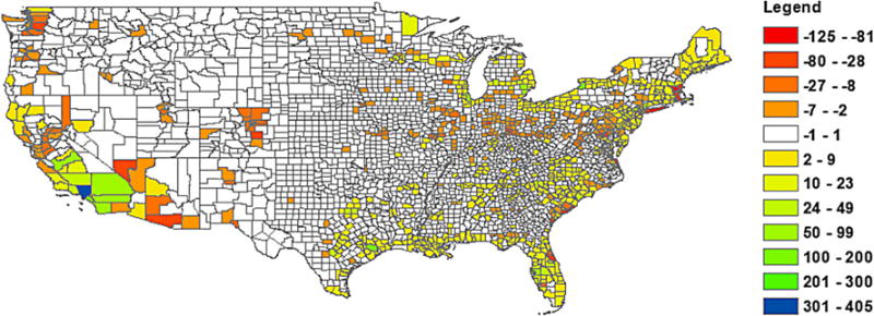
The difference in estimated mortality by county attributed to total PM2.5 between the 2 × 2.5 model and 2 × 2.5 re-gridded resolution
Discussion and conclusions
Using the all-cause mortality risk estimate for PM2.5 from Krewski et al. (2009), we estimate that approximately 142,000 (95 % CI, 97,500–186,400) all-cause deaths occurred in the USA in 2008 due to ambient PM2.5 exposure based on the finest GEOS-Chem model resolution at 0.5 × 0.66°. These deaths account for approximately 6 % (95 % CI 4–8 %) of the national deaths occurring in the USA in 2008. The six species of PM2.5, namely BC, NH4, NIT, SO4, OC, and DST, each cause 9, 14, 22, 22, 28, and 5 % of the total PM2.5 deaths, respectively. Using coarse-model output at 2 × 2.5° produces a national PM2.5 mortality estimate that is 8 % lower than the estimate based on the fine-model results. Since we only include the USA population aged over 30 in our calculation, we are likely to underestimate the mortality attributable to PM2.5, as air pollution likely has adverse health impacts on the population of all ages. The change in mortality estimates when moving from the fine to the coarse-model resolution varies for different species, with the estimates decreasing by 7–18 % for the first five species and increasing by 38 % for DST. Our calculation of the county-level mortality shows that the coarse-model resolution tends to underestimate mortality in counties where large urban centers are located, particularly mortality attributed to primary particulates including BC and OC. On the other hand, deaths due to DST are overestimated by the coarse-model resolution. As we discussed earlier, deaths due to dust are overestimated by the coarse-model resolution mainly owing to the fact that dust concentrations are largely uncorrected with population, whereas concentrations of the other five species tend to be positively corrected with population.
To further explore the effects of coarse resolution on mortality estimates, we scaled modeled concentrations at 0.5 × 0.66° fine resolution to coarser resolution of 1 × 1.25°, 2 × 2.5° and 4 × 5° by simple averaging, a similar approach that was used in Punger and West (2013). The results show that at the 1 × 1.25° resolution, the total PM2.5-related mortality estimate is 4 % lower than the fine resolution (0.5 × 0.66°) estimate, and the 2 × 2.5° and 4 × 5° resolutions produce mortality estimates that are 7 and 15 % lower than the estimate driven with the fine resolution. Furthermore, we found that re-gridded coarse resolutions tend to have the greatest influence (underprediction) on the estimates of national mortality associated with exposure to primary PM2.5 species (BC and OC), whereas the least impact on dust-related mortality estimates.
In comparing the 2 × 2.5 coarse-modeled results with the same resolution re-gridded results, we found that although the re-gridded concentrations produce a national PM2.5-related mortality estimate that is very close to the estimate based on model output, for different species, the differences between the two estimates vary by up to 30 %. Geographically, in the eastern USA and the west coast, the re-gridded output tends to overestimate PM2.5-related mortality whereas in the western USA (except for the west coast), the re-gridded results are likely to underestimate PM2.5 mortality. Ideally, the 2 × 2.5 resolution model provides estimates of average concentrations within each grid cell, which would equal the aggregated, re-gridded results. The differences we see in practice are owing to model resolution error causing these two things to be different. This could be owing to chemistry and/or meteorology. For instance, meteorology would impact the dust emissions, which are a function of the cube of the surface wind speed, which is highly resolution dependent. Also, chemistry might affect the secondary aerosol species. For example, in regions with lots of nitrate, such as the Los Angeles area, large differences in estimated mortality were found (Fig. 7).
Some recent studies investigated how model resolution might affect the calculation of human health impacts associated with PM2.5 exposure. Using modeled concentrations of PM2.5 at the 12-km resolution from CMAQ model and scaling these concentrations to multiple coarser resolutions from 24 to 408 km by simple averaging, Punger and West (2013) found that coarse grid resolutions produce national mortality estimates in the USA that are substantially biased low. In contrast, a regional study on nine regions in the eastern USA, which calculated the human health impacts associated with changes in PM2.5 at 36-, 12-, and 4-km resolutions, found that health impacts associated with changes in concentrations were not sensitive to model resolution (Thompson et al. 2014). Given the conflicting results reported by earlier studies, this study further examines the influence of model resolution on health impact assessment by running a global atmospheric model at a fine and a coarse resolution and also scaling the finest modeled concentrations to coarser resolutions. The results suggest that coarse grid resolutions may produce national mortality estimates that are biased low for PM2.5. Our findings of the influence of resolution on national PM2.5-related mortality estimates are consistent with those of Punger and West (2013). Furthermore, the results of species-specific mortality calculations indicate that coarse resolutions produce larger bias (underestimation) on the mortality associated with primary particles, and may overestimate the mortality due to dust. Also, our analysis of the spatial variations in mortality shows that coarse-model resolutions are most likely to underpredict mortality estimates in large urban centers, such as the Los Angeles metropolitan area, where the greatest numbers of PM2.5-related mortality are predicted.
Despite the uncertainties in our estimates, our findings provide evidence of the bias for quantitative PM2.5 health impact assessment in applications of global atmospheric models where model resolutions are likely to be restricted by computational power and other factors. Future studies should extend this analysis to larger geographical regions to examine the influence of resolution at a larger scale. Moreover, future studies may consider applying different concentration-response coefficients to various PM2.5 species to reflect species potency. Doing so would further differentiate the impacts of model resolution on the estimates of burden of different species on public health.
Acknowledgments
This research is supported through NASA Applied Sciences Program grant NNX09AN77G. Dr. Ying Li was partially supported by a postdoctoral fellowship from the Earth Institute at Columbia University.
Appendix
Table 4.
Comparing national mortality estimates attributable to each PM2.5 species based on modeled 0.5 × 0.66° concentrations using two approaches: (1) directly applying the simulated annual average concentrations of each species (approach used in this study) and (2) calculating mortality for the total PM2.5 concentration relative to the total PM2.5 minus one species (Punger and West 2013)
| Species | National mortality
|
Percent difference: (2) relative to (1) | |
|---|---|---|---|
| Approach (1) | Approach (2) | ||
| BC | 13,280 | 12,379 | −6.8 % |
| NH4 | 20,464 | 19,191 | −6.2 % |
| NIT | 32,683 | 30,864 | −5.6 % |
| SO4 | 32,539 | 30,772 | −5.4 % |
| OC | 40,144 | 38,064 | −5.2 % |
| DST | 7372 | 6997 | −5.1 % |
| Sum of six species | 146,482 | 138,267 | −5.6 % |
Table 4 shows that our approach produces mortality estimates for the six species that are slightly higher (approximately 5–7 %) than those based on the Punger and West approach. The total PM2.5-related mortality calculated using PM2.5 concentrations is 142,342 (Table 2). Therefore, when comparing the summary of mortality due to the six species with the total PM2.5 deaths calculated using PM2.5 concentrations directly, the estimate based on our approach is 2.9 % higher whereas the estimate based on the Punger and West approach is 2.9 % lower
Fig. 8.
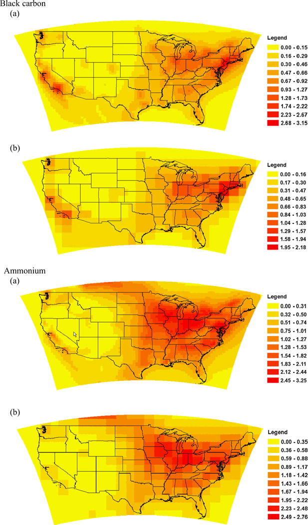
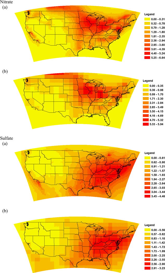

Modeled annual average PM2.5 species concentrations in 2008 using GEOS-Chem output at a fine (0.5 × 0.66°) resolution and b coarse (2 × 2.5°) resolution (unit, μg/m3)
Fig. 9.
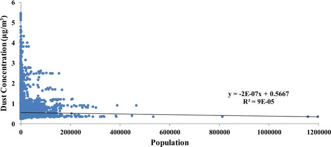
Correlation analysis of the dust concentration and population using fine (0.5 × 0.66°) model results
Fig. 10.
The difference in estimated mortality by county attributed to total PM2.5 between the fine-model resolution (0.5 × 0.66°) and the coarse resolution (2 × 2.5°)
Fig. 11.
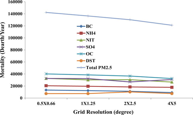
a Estimates of national all-cause mortality due to PM2.5 species at various grid resolutions, including the fine-model resolution (0.5 × 0.66°) and three re-gridded resolution (1 × 1.25, 2 × 2.5, and 4 × 5)
Contributor Information
Ying Li, Department of Environmental Health, College of Public Health, East Tennessee State University, PO Box 70682, Johnson City, TN, USA.
Daven K. Henze, Department of Mechanical Engineering, University of Colorado at Boulder, 1111 Engineering Drive UCB 427, Boulder, CO, USA
Darby Jack, Department of Environmental Health Sciences, Mailman School of Public Health, Columbia University, 722 West 168th Street, New York, NY, USA.
Patrick L. Kinney, Department of Environmental Health Sciences, Mailman School of Public Health, Columbia University, 722 West 168th Street, New York, NY, USA
References
- Abt Associates I. Environmental Benefits and Mapping Program. 2013 BenMAP, Version 4.0.67. [Google Scholar]
- Alexander B, et al. Sulfate formation in sea-salt aerosols: constraints from oxygen isotopes. J Geophys Res Atenos. 2005:1984–2012. 110. [Google Scholar]
- Anenberg SC, Horowitz LW, Tong DQ, West J. An estimate of the global burden of anthropogenic ozone and fine particulate matter on premature human mortality using atmospheric modeling. Environ Health Perspect. 2010;118:1189–1195. doi: 10.1289/ehp.0901220. [DOI] [PMC free article] [PubMed] [Google Scholar]
- Anenberg SC, et al. Global air quality and health co-benefits of mitigating near-term climate change through methane and black carbon emission controls. 2012 doi: 10.1289/ehp.1104301. [DOI] [PMC free article] [PubMed] [Google Scholar]
- Arunachalam S, Wang B, Davis N, Baek BH, Levy JI. Effect of chemistry-transport model scale and resolution on population exposure to PM2.5 from aircraft emissions during landing and takeoff. Atenos Environ. 2011;45:3294–3300. doi: 10.1016/j.atmosenv.2011.03.029. [DOI] [Google Scholar]
- Beelen R, et al. Long-term effects of traffic-related air pollution on mortality in a Dutch cohort (NLCS-AIR study) Environ Health Perspect. 2008;116:196–202. doi: 10.1289/ehp.10767. [DOI] [PMC free article] [PubMed] [Google Scholar]
- Bey I, et al. Global modeling of tropospheric chemistry with assimilated meteorology: model description and evaluation. J Geophys Res Atenos (1984–2012) 2001;106:23073–23095. [Google Scholar]
- Bond TC, et al. Historical emissions of black and organic carbon aerosol from energy-related combustion, 1850–2000. Glob Biogeochem Cycles. 2007;21 [Google Scholar]
- Burnett RT, et al. An integrated risk function for estimating the global burden of disease attributable to ambient fine particulate matter exposure. 2014 doi: 10.1289/ehp.1307049. [DOI] [PMC free article] [PubMed] [Google Scholar]
- Chen D, Wang Y, McElroy M, He K, Yantosca R, Sager PL. Regional CO pollution and export in China simulated by the high-resolution nested-grid GEOS-Chem model. Atenos Chem Phys. 2009;9:3825–3839. [Google Scholar]
- Cohen AJ, et al. The global burden of disease due to outdoor air pollution. J Toxic Environ Health A. 2005;68:1301–1307. doi: 10.1080/15287390590936166. [DOI] [PubMed] [Google Scholar]
- Cooke W, Liousse C, Cachier H, Feichter J. Construction of a 1 × 1 fossil fuel emission data set for carbonaceous aerosol and implementation and radiative impact in the ECHAM4 model. J Geophys Res Atmos (1984–2012) 1999;104:22137–22162. [Google Scholar]
- Daniels MJ, Dominici F, Samet JM, Zeger SL. Estimating particulate matter-mortality dose-response curves and threshold levels: an analysis of daily time-series for the 20 largest US cities. Am J Epidemiol. 2000;152:397–406. doi: 10.1093/aje/152.5.397. [DOI] [PubMed] [Google Scholar]
- De Meij A, Wagner S, Cuvelier C, Dentener F, Gobron N, Thunis P, Schaap M. Model evaluation and scale issues in chemical and optical aerosol properties over the greater Milan area (Italy), for June 2001. Atmos Res. 2007;85:243–267. [Google Scholar]
- Dockery DW, et al. An association between air pollution and mortality in six US cities. N Engl J Med. 1993;329:1753–1759. doi: 10.1056/NEJM199312093292401. [DOI] [PubMed] [Google Scholar]
- Duncan Fairlie T, Jacob DJ, Park RJ. The impact of transpacific transport of mineral dust in the United States. Atmos Environ. 2007;41:1251–1266. [Google Scholar]
- Dunlea E, et al. Evolution of Asian aerosols during transpacific transport in INTEX-B. Atmos Chem Phys. 2009;9:7257–7287. [Google Scholar]
- EPA U. Guidance on the use of models and other analyses for demonstrating attainment of air quality goals for ozone, M2. 5, and regional haze. US Environmental Protection Agency, Office of Air Quality Planning and Standards; 2007. [Google Scholar]
- EPA US. Report to congress on black carbon. 2012 EPA-450/R-12-001. [Google Scholar]
- Farm N, Lamson AD, Anenberg SC, Wesson K, Risley D, Hubbell BJ. Estimating the national public health burden associated with exposure to ambient PM2. 5 and ozone. Risk Anal. 2012;32:81–95. doi: 10.1111/j.1539-6924.2011.01630.x. [DOI] [PubMed] [Google Scholar]
- Farm N, Fulcher CM, Baker K. The recent and future health burden of air pollution apportioned across US sectors. Environ Sci Technol. 2013;47:3580–3589. doi: 10.1021/es304831q. [DOI] [PubMed] [Google Scholar]
- Filleul L, et al. Twenty five year mortality and air pollution: results from the French PAARC survey. Occup Environ Med. 2005;62:453–460. doi: 10.1136/oem.2004.014746. [DOI] [PMC free article] [PubMed] [Google Scholar]
- Fisher JA, et al. Sources, distribution, and acidity of sulfate-ammonium aerosol in the Arctic in winter-spring. Atmos Environ. 2011;45:7301–7318. [Google Scholar]
- Fountoukis C, Nenes A. ISORROPIA II: a computationally efficient thermodynamic equilibrium model for K+−Ca 2+−Mg 2+−NH 4+−Na+−SO42−NO3−Cl−H2O aerosols. Atmos Chem Phys. 2007;7:4639–4659. [Google Scholar]
- Generoso S, Bey I, Labonne M, Bréon FM. Aerosol vertical distribution in dust outflow over the Atlantic: comparisons between GEOS-Chem and Cloud-aerosol Lidar and Infrared Pathfinder Satellite Observation (CALIPSO) J Geophys Res Atmos. 2008:1984–2012. 113. [Google Scholar]
- Giglio L, Randerson J, Van der Werf G, Kasibhatla P, Collatz G, Morton D, DeFries R. Assessing variability and long-term trends in burned area by merging multiple satellite fire products. Biogeosciences. 2010;7:1171–1186. [Google Scholar]
- Heald CL, Ridley DA, Kreidenweis SM, Drury EE. Satellite observations cap the atmospheric organic aerosol budget. Geophys Res Lett. 2010;37 [Google Scholar]
- Heald CL, et al. Exploring the vertical profile of atmospheric organic aerosol: comparing 17 aircraft field campaigns with a global model. Atmos Chem Phys. 2011;11:12673–12696. [Google Scholar]
- Heald CL, et al. Atmospheric ammonia and particulate inorganic nitrogen over the United States. Atmos Chem Phys Discuss. 2012;12 [Google Scholar]
- Henze DK, Seinfeld JH, Shindell DT. Inverse modeling and mapping US air quality influences of inorganic PM 2.5 precursor emissions using the adjoint of GEOS-Chem. Atmos Chem Phys. 2009;9:5877–5903. [Google Scholar]
- Jaeglé L, Quinn P, Bates T, Alexander B, Lin J-T. Global distribution of sea salt aerosols: new constraints from in situ and remote sensing observations. Atmos Chem Phys. 2011;11:3137–3157. [Google Scholar]
- Janssen N, et al. Black carbon as an additional indicator of the adverse health effects of airborne particles compared with PM10 and PM2. 5. Environ Health Perspect. 2011;119:1691–1699. doi: 10.1289/ehp.1003369. [DOI] [PMC free article] [PubMed] [Google Scholar]
- Jimenez J, et al. Evolution of organic aerosols in the atmosphere. Science. 2009;326:1525–1529. doi: 10.1126/science.1180353. [DOI] [PubMed] [Google Scholar]
- Johnson MS, Meskhidze N, Praju Kiliyanpilakkil V. A global comparison of GEOS-Chem-predicted and remotely-sensed mineral dust aerosol optical depth and extinction profiles. J Adv Model Earth Syst. 2012;4 [Google Scholar]
- Kheirbek I, Wheeler K, Walters S, Kass D, Matte T. PM2. 5 and ozone health impacts and disparities in New York City: sensitivity to spatial and temporal resolution. Air Qual Atmos Health. 2013;6:473–486. doi: 10.1007/s11869-012-0185-4. [DOI] [PMC free article] [PubMed] [Google Scholar]
- Krewski D, et al. Extended follow-up and spatial analysis of the American Cancer Society study linking particulate air pollution and mortality. Vol. 140. Health Effects Institute; Boston: 2009. [PubMed] [Google Scholar]
- Laden F, Schwartz J, Speizer FE, Dockery DW. Reduction in fine particulate air pollution and mortality: extended follow-up of the Harvard Six Cities study. Am J Respir Crit Care Med. 2006;173:667–672. doi: 10.1164/rccm.200503-443OC. [DOI] [PMC free article] [PubMed] [Google Scholar]
- Li Y, Crawford-Brown DJ. Assessing the co-benefits of greenhouse gas reduction: health benefits of particulate matter related inspection and maintenance programs in Bangkok, Thailand. Sci Total Environ. 2011;409:1774–1785. doi: 10.1016/j.scitotenv.2011.01.051. [DOI] [PubMed] [Google Scholar]
- Li Y, et al. Burden of disease attributed to anthropogenic air pollution in the United Arab Emirates: estimates based on observed air quality data. Sci Total Environ. 2010;408:5784–5793. doi: 10.1016/j.scitotenv.2010.08.017. [DOI] [PubMed] [Google Scholar]
- Liao K-J, et al. Sensitivities of ozone and fine particulate matter formation to emissions under the impact of potential future climate change. Environ Sci Technol. 2007;41:8355–8361. doi: 10.1021/es070998z. [DOI] [PubMed] [Google Scholar]
- Lim SS, et al. A comparative risk assessment of burden of disease and injury attributable to 67 risk factors and risk factor clusters in 21 regions, 1990–2010: a systematic analysis for the Global Burden of Disease Study 2010. Lancet. 2013;380:2224–2260. doi: 10.1016/S0140-6736(12)61766-8. [DOI] [PMC free article] [PubMed] [Google Scholar]
- Liu H, Jacob DJ, Bey I, Yantosca RM. Constraints from 210Pb and 7Be on wet deposition and transport in a global three-dimensional chemical tracer model driven by assimilated meteorological fields. J Geophys Res Atmos (1984–2012) 2001;106:12109–12128. [Google Scholar]
- Luan Y, Jaeglé L. Composite study of aerosol export events from East Asia and North America. Atmos Chem Phys. 2013;13:1221–1242. doi: 10.5194/acp-13-1221-2013. [DOI] [Google Scholar]
- Mao J, Fan S, Jacob D, Travis K. Radical loss in the atmosphere from Cu-Fe redox coupling in aerosols. Atmos Chem Phys. 2013;13:509–519. [Google Scholar]
- Mensink C, De Ridder K, Deutsch F, Lefebre F, Van de Vel K. Examples of scale interactions in local, urban, and regional air quality modelling. Atmos Res. 2008;89:351–357. doi: 10.1016/j.atmosres.2008.03.020. [DOI] [Google Scholar]
- Olivier JG, Van Aardenne JA, Dentener FJ, Pagliari V, Ganzeveld LN, Peters JA. Recent trends in global greenhouse gas emissions: regional trends 1970–2000 and spatial distribution of key sources in 2000. Environ Sci. 2005;2:81–99. [Google Scholar]
- Ostro B. Outdoor air pollution WHO Environmental burden of disease series. 2004 doi: 10.1080/15287390590936166. [DOI] [PubMed] [Google Scholar]
- Park RJ, Jacob DJ, Chin M, Martin RV. Sources of carbonaceous aerosols over the United States and implications for natural visibility. J Geophys Res Atmos. 2003:1984–2012. 108. [Google Scholar]
- Park RJ, Jacob DJ, Field BD, Yantosca RM, Chin M. Natural and transboundary pollution influences on sulfate-nitrate-ammonium aerosols in the United States: implications for policy. J Geophys Res Atmos. 2004:1984–2012. 109. [Google Scholar]
- Philip S, Martin RV, van Donkelaar A, Lo JW-H, Wang Y, Chen D, Zhang L, Kasibhatla PS, Wang S, Zhang Q, Lu Z, Streets DG, Bittman S, Macdonald DJ. Global chemical composition of ambient fine particulate matter estimated from satellite observations and a chemical transport model environmental health perspectives. 2014 doi: 10.1021/es502965b. Submitted. [DOI] [PMC free article] [PubMed] [Google Scholar]
- Pope CA. Invited commentary: particulate matter-mortality exposure-response relations and threshold. Am J Epidemiol. 2000;152:407–412. doi: 10.1093/aje/152.5.407. [DOI] [PubMed] [Google Scholar]
- Pope CA, III, Thun MJ, Namboodiri MM, Dockery DW, Evans JS, Speizer FE, Heath CW., Jr Particulate air pollution as a predictor of mortality in a prospective study of US adults. Am J Respir Crit Care Med. 1995;151:669–674. doi: 10.1164/ajrccm/151.3_Pt_1.669. [DOI] [PubMed] [Google Scholar]
- Pope CA, III, Burnett RT, Thun MJ, Calle EE, Krewski D, Ito K, Thurston GD. Lung cancer, cardiopulmonary mortality, and long-term exposure to fine particulate air pollution. JAMA. 2002;287:1132–1141. doi: 10.1001/jama.287.9.1132. [DOI] [PMC free article] [PubMed] [Google Scholar]
- Punger EM, West JJ. The effect of grid resolution on estimates of the burden of ozone and fine particulate matter on premature mortality in the USA. Air Qual Atmos Health. 2013;6:563–573. doi: 10.1007/s11869-013-0197-8. [DOI] [PMC free article] [PubMed] [Google Scholar]
- Schwartz J, Laden F, Zanobetti A. The concentration-response relation between PM (2.5) and daily deaths. Environ Health Perspect. 2002;110:1025. doi: 10.1289/ehp.021101025. [DOI] [PMC free article] [PubMed] [Google Scholar]
- Smith KR, et al. Public health benefits of strategies to reduce greenhouse-gas emissions: health implications of short-lived greenhouse pollutants. Lancet. 2010;374:2091–2103. doi: 10.1016/S0140-6736(09)61716-5. [DOI] [PMC free article] [PubMed] [Google Scholar]
- Streets DG, et al. Revisiting China’s CO emissions after the Transport and Chemical Evolution over the Pacific (TRACE-P) mission: synthesis of inventories, atmospheric modeling, and observations. J Geophys Res Atmos. 2006:1984–2012. 111. [Google Scholar]
- Thompson TM, Saari RK, Selin NE. Air quality resolution for health impact assessment: influence of regional characteristics. Atmos Chem Phys. 2014;14:969–978. doi: 10.5194/acp-14-969-2014. [DOI] [Google Scholar]
- van der Werf GR, et al. Global fire emissions and the contribution of deforestation, savanna, forest, agricultural, and peat fires (1997–2009) Atmos Chem Phys. 2010;10:11707–11735. [Google Scholar]
- van Donkelaar A, et al. Analysis of aircraft and satellite measurements from the Intercontinental Chemical Transport Experiment (INTEX-B) to quantify long-range transport of East Asian sulfur to Canada. Atmos Chem Phys. 2008;8:2999–3014. [Google Scholar]
- van Donkelaar A, Martin RV, Brauer M, Kahn R, Levy R, Verduzco C, Villeneuve PJ. Global estimates of ambient fine particulate matter concentrations from satellite-based aerosol optical depth: development and application. Environ Health Perspect. 2010;118:847. doi: 10.1289/ehp.0901623. [DOI] [PMC free article] [PubMed] [Google Scholar]
- Walker J, Philip S, Martin R, Seinfeld J. Simulation of nitrate, sulfate, and ammonium aerosols over the United States. Atmos Chem Phys. 2012;12:11213–11227. [Google Scholar]
- Wang X, Mauzerall DL. Evaluating impacts of air pollution in China on public health: implications for future air pollution and energy policies. Atmos Environ. 2006;40:1706–1721. [Google Scholar]
- Wang YX, McElroy MB, Jacob DJ, Yantosca RM. A nested grid formulation for chemical transport over Asia: applications to CO. J Geophys Res Atmos. 2004:1984–2012. 109. [Google Scholar]
- Wesely M. Parameterization of surface resistances to gaseous dry deposition in regional-scale numerical models. Atmos Environ (1967) 1989;23:1293–1304. [Google Scholar]
- West JJ, Fiore AM, Horowitz LW, Mauzerall DL. Global health benefits of mitigating ozone pollution with methane emission controls. Proc Natl Acad Sci U S A. 2006;103:3988–3993. doi: 10.1073/pnas.0600201103. [DOI] [PMC free article] [PubMed] [Google Scholar]
- Zhang L, et al. Nitrogen deposition to the United States: distribution, sources, and processes. Atmos Chem Phys Discuss. 2012;12:241–282. [Google Scholar]
- Zhang L, Kok JF, Henze DK, Li Q, Zhao C. Improving simulations of fine dust surface concentrations over the western United States by optimizing the particle size distribution. Geophys Res Lett. 2013;40:3270–3275. [Google Scholar]
- Zhu L, et al. Constraining US ammonia emissions using TES remote sensing observations and the GEOS-Chem adjoint model. J Geophys Res Atmos. 2013;118:3355–3368. [Google Scholar]