

Abstract
Diffusion MRI has been proposed as a non‐invasive technique for axonal diameter mapping. However, accurate estimation of small diameters requires strong gradients, which is a challenge for the transition of the technique from preclinical to clinical MRI scanners, since these have weaker gradients. In this work, we develop a framework to estimate the lower bound for accurate diameter estimation, which we refer to as the resolution limit. We analyse only the contribution from the intra‐axonal space and assume that axons can be represented by impermeable cylinders. To address the growing interest in using techniques for diffusion encoding that go beyond the conventional single diffusion encoding (SDE) sequence, we present a generalised analysis capable of predicting the resolution limit regardless of the gradient waveform. Using this framework, waveforms were optimised to minimise the resolution limit. The results show that, for parallel cylinders, the SDE experiment is optimal in terms of yielding the lowest possible resolution limit. In the presence of orientation dispersion, diffusion encoding sequences with square‐wave oscillating gradients were optimal. The resolution limit for standard clinical MRI scanners (maximum gradient strength 60–80 mT/m) was found to be between 4 and 8 μm, depending on the noise levels and the level of orientation dispersion. For scanners with a maximum gradient strength of 300 mT/m, the limit was reduced to between 2 and 5 μm.
Keywords: Axon diameter, diffusion imaging, double diffusion encoding, microstructure, oscillating diffusion encoding, q‐trajectory encoding, resolution limit, single diffusion encoding
Abbreviations used
- DDE
double diffusion encoding
- dMRI
diffusion MRI
- FWHM
full width at half‐maximum
- GPD
Gaussian phase distribution
- IVIM
intra‐voxel incoherent motion
- OGSE
oscillating gradient spin echo
- SDE
single diffusion encoding
- SNR
signal‐to‐noise ratio
- QTE
q‐trajectory encoding.
1. INTRODUCTION
Axons in the white matter serve as the backbone of the brain network. The information transmission through this network is determined by the conduction velocity along the axons and the axon density, which both depend on the axon diameter.1, 2, 3 Non‐invasive methods to determine the axon diameter and the axon density are thus important for mapping the network of the brain.
Most axons have diameters between 0.2 and 20 μm.4 Large axons facilitate rapid communication, e.g. for processing of sensorimotor stimuli, and are found in structures such as the corticospinal tract and the midbody of the corpus callosum. However, large axons occupy much space, yielding low axon density, and demand much energy per bit of information transmitted.5 Smaller axons, with a diameter of 0.7 μm, minimise the energy cost per bit.5 Not surprisingly, smaller axons are the most prevalent in the brain and fewer than 1% of its axons are larger than 3 μm.6 In the optic nerve, most axons have diameters below 2 μm, with a peak of 0.7 μm.5
Diffusion magnetic resonance imaging (dMRI) may enable model‐based estimation of compartment sizes and densities.7, 8 For example, Assaf et al. investigated fixed nerves and demonstrated that the average displacement of water molecules due to diffusion is limited to approximately 2 μm in the direction perpendicular to a coherent nerve fiber structure.9 By modelling the axons as cylinders and extra‐axonal water as undergoing Gaussian diffusion, the full axon diameter distribution has been recovered from dMRI data.10, 11
Techniques for axon diameter mapping have been developed in systems capable of producing magnetic field gradients of up to 1500 mT/m,10 but human MRI scanners feature gradients with much lower amplitudes. Conventional clinical systems can deliver gradients of up to 80 mT/m, and custom systems such as the Connectom system can reach as high as 300 mT/m.12 The gradient amplitude is important, because it defines the so‐called resolution limit in diffusion MRI.13, 14 The emergence of this limit is obvious in q‐space diffusion MRI, where sizes are obtained from the width of the so‐called ensemble average propagator.9, 15, 16 This propagator is obtained by means of an inverse Fourier transform of the signal‐versus‐q curve.15 However, limited gradient performance leads to limited support in terms of high q‐values, and thus the resulting propagator is convolved with a low‐pass kernel with a width defined by the inverse of the gradient amplitude.14 As the true size goes towards zero, the size estimated from the width of the estimated propagator remains at the width of the kernel. Weaker gradients result in a wider kernel, and thereby a poorer resolution in terms of a higher value of the resolution limit. The gradient amplitude can thus be compared with the wavelength of light in optical microscopy, which defines the resolution in terms of the Abbe diffraction limit.17, 18 Coincidentally, this limit prevents accurate quantification of axon diameters below approximately 0.4 μm with conventional light microscopy.19
The resolution limit is important, not only in q‐space dMRI but also for model‐based recovery of the axon diameter.8 Approaches such as CHARMED, AxCaliber, and ActiveAx estimate the axon diameter by solving an inverse problem in which axons are modelled as straight cylinders.10, 20, 21 Specificity to the axon diameter is assumed to be obtained from the signal attenuation of intra‐axonal water; however, the sensitivity of the MR signal to small cylinder diameters is low, because a small change in the diameter produces a negligible change in the measured signal. Hence, small cylinder diameters are challenging to estimate accurately (for example, see Figure 1a–d of Dyrby et al.22). In other words, cylinders with a diameter below the resolution limit are indistinguishable from virtual cylinders with a diameter of zero. Preliminary results assuming parallel cylinders indicated that the resolution limit is approximately 6 μm for gradient amplitudes of 60 mT/m and 3 μm for amplitudes of 300 mT/m.23 More realistic cases including orientation dispersion may result in even lower sensitivity to the diameter24 and cause further complications for solving the inverse problem and interpreting its solution.25, 26, 27
Most diameter mapping studies have employed the Stejskal–Tanner experiment,28 here referred to as the single diffusion encoding (SDE) experiment following the nomenclature in Shemesh et al.29 Diffusion‐encoding techniques that go beyond SDE have recently been proposed as potential solutions to reduce the resolution limit. Such techniques have generally been adapted from the fields of porous materials research, and include the double diffusion encoding (DDE) sequence,30, 31, 32, 33, 34 oscillating diffusion encoding (ODE), also known as oscillating gradient spin echo (OGSE) or modulated‐gradient NMR,24, 35, 36, 37, 38, 39 and non‐pulsed and non‐parametric gradient waveforms,40, 41 which we refer to as q‐trajectory encoding (QTE).42 In combination with improved gradient hardware for clinical MRI,43 gradient waveforms beyond SDE may enable non‐invasive recovery of the axon diameter.
In this work, we introduce an analytical framework to predict the resolution limit for any gradient waveform. Prior approaches in this direction were fully numerical, and confined to the SDE and ODE sequences.24 We analyse three cases: the first where axons are parallel, the second where there is full axonal orientation dispersion, and the third where there is partial alignment. We limit our investigation to estimation of the diameter from intra‐axonal water diffusion, assuming axons can be modelled by impermeable and straight cylinders. Provided this assumption holds, which can be debated,27 our results can be used directly in the analysis of measurements on intra‐axonal metabolites.44 For water measurements, contributions from extra‐axonal components must be incorporated in the analysis. Such components are often assumed to exhibit Gaussian diffusion,20, 21 which may not be congruent with the physics of extracellular diffusion.45 Accounting for time‐dependent diffusion outside axons is likely needed for accurate mapping of axonal characteristics,46, 47 but investigating its impact on the resolution limit was beyond the scope of the present study. Our analysis nevertheless contributes with a lower bound on the resolution limit of the intra‐axonal component.
2. THEORY
We express the attenuation of the signal due to diffusion perpendicular to the main axis of a cylinder as S(b|d), where b refers to the diffusion encoding strength (b‐value) and d to the cylinder diameter. We will use this notation to derive the resolution limit ( ), which we define as the diameter where the signal attenuation is indistinguishable from the case where the diameter goes towards zero,
| (1) |
We will derive the value of for three cases: parallel cylinders, randomly ordered cylinders, and finally for any level of orientation dispersion. We assume all cylinders to be equal in size. We limit the analysis to one‐dimensional (1D) waveforms, like those applied in SDE and ODE, but the analysis is applicable also to 1D aspects of multi‐dimensional diffusion encoding, such as DDE or QTE. For all waveforms, note that g(t) must fulfil the condition
| (2) |
in order to form an echo at the centre of k‐space. Here and throughout the analysis, we will assume g(t) to describe the effective gradient waveform after effects of RF pulses have been accounted for.
2.1. Defining the resolution limit
To define the resolution limit, we begin by defining the difference in signal (ΔS) between cylinders with a diameter approaching zero and those with a diameter corresponding to the resolution limit,
| (3) |
We formally define the resolution limit as a hypothesis test of whether the observed ΔS is statistically higher than zero. Assuming that, due to noise, ΔS is normally distributed,48 we phrase the test in terms of a requirement on the z‐score z(ΔS)⩾z α, where z α is the z‐threshold for significance level α and
| (4) |
and σ is the standard deviation of the signal due to noise, defined from the signal‐to‐noise ratio (SNR) and the signal amplitude at b=0(S 0) according to SNR=S 0/σ. Moreover, n is the number of signal averages. Deriving d from a model fitted to data acquired with multiple values of b would improve precision and be similar to increasing n, although it would be less efficient than sampling with just b = 0 and .49
Altogether, this yields a requirement for the normalised signal at the resolution limit:
| (5) |
and
| (6) |
If the attenuation ΔS/S 0 is less than , it will be indistinguishable from zero, i.e. the attenuation would be identical to that from a cylinder with a diameter of zero. In other words, the diameter would be below the resolution limit. When fitting models to measurements in systems with structures having sizes below the resolution limit, the diameter should not be a free model parameter. Exploiting the resolution limit thus allows for model simplifications, such as using ‘stick’ diffusion tensors with zero radial diffusivity and non‐zero axial diffusivity to model diffusion inside thin axons.26, 50
In this study, we set z α to 1.64 for a one‐sided test at the 5% significance level. For a SNR of 50 (σ=S 0/SNR) and n=10, we obtain . For completeness, note that for SNR = 30 and n=1. Throughout this work, we will use the level = 1% as a reference. This is a reasonable lower limit for in vivo measurements on a clinical MRI system. Although smaller effects are detectable in principle, in practice they may be difficult to separate from effects not accounted for in the model, for example residual eddy currents,51 or effects that may be difficult to model accurately for non‐SDE waveforms, such as intra‐voxel incoherent motion (IVIM).52 In other words, effects smaller than 1% may be statistically significant but practically irrelevant.
In order to derive the resolution limit, we consider the attenuation for diffusion encoded in a direction perpendicular to a cylinder, given by
| (7) |
where D ⊥ is the apparent radial diffusivity, which depends on d as well as on the timing of the gradient waveform used for the diffusion encoding. The approximation of the exponential is valid where the attenuation factor b D ⊥ is small, which is true per definition at the resolution limit. Since , the expression for ΔS in Equation 3 is reduced to
| (8) |
2.2. Parallel cylinders
We begin by deriving the resolution limit for parallel cylinders, first for the SDE sequence and then for the case of arbitrary gradient waveforms.
2.2.1. Single diffusion encoding sequence
Three parameters define an SDE experiment: the duration and leading‐edge separation of the gradient pulses (δ and Δ, respectively), and the gradient amplitude (g). How should these three parameters be selected in order to minimise ? The question is equivalent to maximising ΔS≈b D(δ,Δ|d), where D(·) depends on the timing variables δ and Δ,
| (9) |
and γ is the gyromagnetic ratio. Since b, and thus ΔS, increases monotonically with g, the gradient should assume its maximal value in order to minimise . In order to select the timing parameters that minimise , we express D ⊥ using the Gaussian phase distribution (GPD) approximation,53, 54 according to
| (10) |
where k(α,β) is defined in the Appendix, D 0 is the free diffusivity of the intra‐cylinder water, and
| (11) |
From Equations 8, 9, and 10, we obtain
| (12) |
According to numerical computations, this expression is maximised when δ=Δ, or expressed in unitless variables when α=β. Moreover, close to the resolution limit, where d is small, α≫1. Under these conditions, we can approximate D ⊥ as55, 56
| (13) |
Hence
| (14) |
This expression can be used to estimate cylinder diameters, assuming intra‐axonal‐specific data are acquired, and with prior knowledge of D 0. Potential errors in the assumed value of D 0 are not critical, since errors of up to 50 % in D 0 give at most 10–15% errors in d. The expression in Equation 14 also gives the resolution limit for parallel cylinders and SDE, according to
| (15) |
For , g=80 mT/m, and δ=40 ms, we obtain for the high‐SNR case where and when . Since D 0 decreases with temperature, investigations of cold fixed tissue may be beneficial to reduce the resolution limit.
2.2.2. Spectral domain analysis of restricted diffusion
In the previous section, we derived the resolution limit for the SDE sequence. However, gradient waveforms other than SDE may offer improved sensitivity to small cylinders. In order to investigate arbitrary gradient waveforms, we analyse the diffusion process in the spectral domain,57 where the effect of diffusion encoding on the normalised signal (S/S 0) is given by
| (16) |
where D(ω) is the diffusion spectrum and q(ω) is the Fourier transform of q(t), defined by
| (17) |
For completeness, we note that
| (18) |
where f is the frequency measured in Hertz (2πf=ω). For convenience, we will use both ω and f. The relation in Equation 18 is also known as Parseval's identity. For free diffusion, D(ω)=D 0, and thus Equation 16 evaluates to .
For restricted diffusion in a cylinder, as well as for diffusion between parallel plates or in spherical geometries, the diffusion encoding spectrum D(ω) can be described by a sum of Lorenzian functions57:
| (19) |
where C i and b i are coefficients that depend on the geometry and are defined for a cylinder geometry in the Appendix. The Appendix also shows the derivation of this specific form of Equation 19 from the expression in Equation (36) of Stepisnik.57
For low frequencies, D(ω) can be approximated by a second‐order polynomial47, 57, 58
| (20) |
where k=7/1536. This approximation yields reasonably accurate signal predictions as long as the diffusion encoding spectrum has negligible power for frequencies above a cut‐off frequency f 0. The difference between the true spectrum and the approximation is less than 20% as long as , which can also be seen in Figure 1. This inequality can be used to define f 0 according to
| (21) |
For and d=2μm, we obtain f 0≈500 Hz. For reference, note that the maximal frequency of a sine or cosine wave that utilises the maximal gradient amplitude is given by , which equates to approximately 400 Hz for a high‐performance clinical scanner with mT/m/ms and mT/m. As a consequence, the approximation in Equation 20 can be used in Equation 16 to predict the signal with reasonable accuracy for many of the waveforms that are useful in practice.
Figure 1.
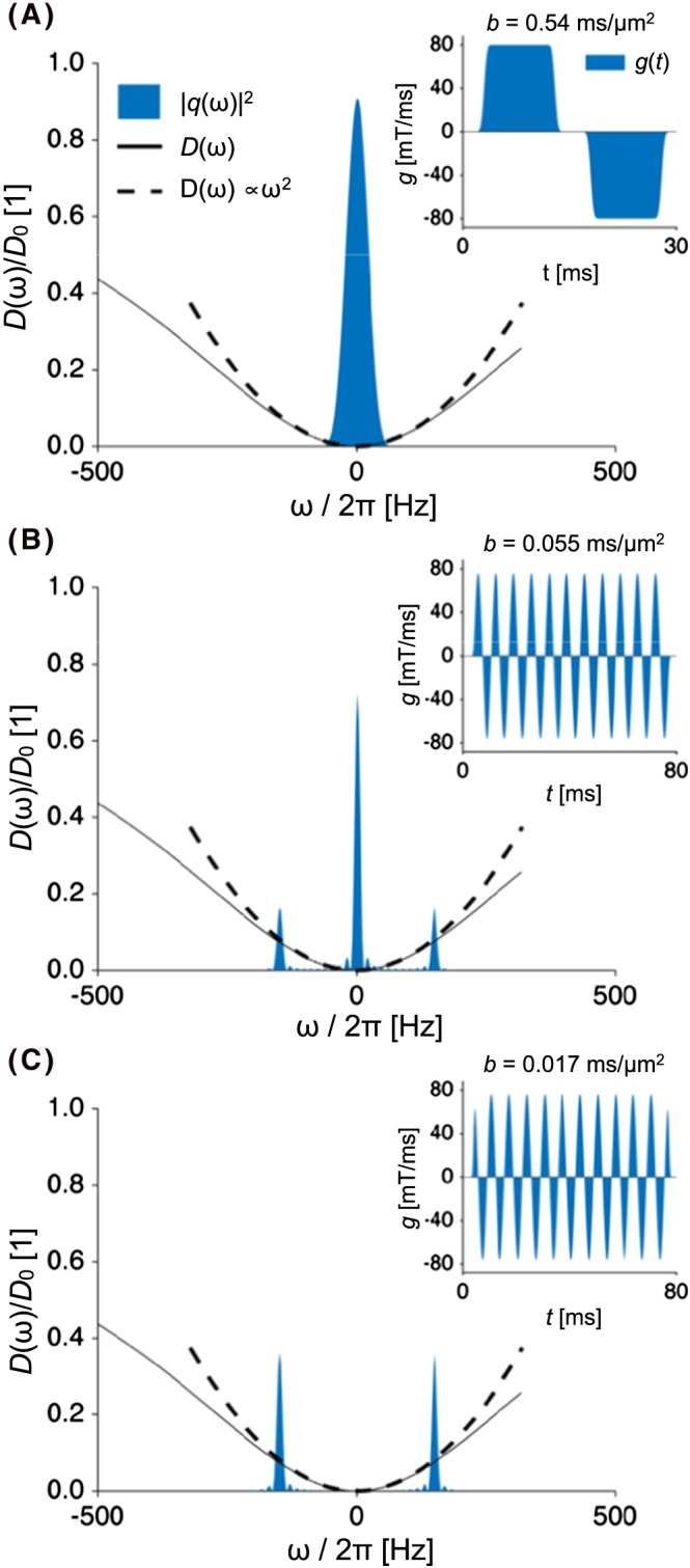
Diffusion and encoding spectra, shown by black lines and blue areas. The dashed line shows the low‐frequency approximation. The spectra were generated for d=3μm and , and were normalised by the bulk diffusivity (D 0). Insets show gradient waveforms (g) generated for an SDE experiment with δ=10 ms and Δ=15 ms in panel A, with a sine wave with f=150 Hz in panel B, and a cosine wave (f=150 Hz) in panel C. The b‐values for these waveforms were 0.5, 0.05, and 0.017 ms/μm2
2.2.3. Resolution limit for parallel axons and general waveforms
A key result of the present analysis concerns the implications of the low‐frequency approximation for the resolution limit. Following Equations 7, 16, and 20, we obtain
| (22) |
An important feature of this relation is that it separates the effects of the geometry (d 4) from the diffusion encoding (the integral part). By utilising Parseval's identity and Equation 22, we can simplify the integral further:
| (23) |
We use this result to define an important entity:
| (24) |
where
| (25) |
since
| (26) |
We refer to the entity V ω as the ‘spectral encoding variance’, since it is defined from the second moment of q(ω). The unit of V ω is 1/s2.
The product b V ω captures all features of the gradient waveforms required to predict the signal attenuation perpendicular to the cylinder. The b‐value captures the attenuation and V ω the time‐dependence, since we can approximate D ⊥ for an arbitrary gradient waveform by
| (27) |
The signal attenuation is thus approximated by
| (28) |
The expression above can be shown to be equivalent to Equation (119) of Grebenkov,59 which was derived for diffusion in the motional narrowing regime. Previous work on the motional narrowing regime in the context of spin relaxation has found similar equations relating the square of the gradient field, the compartment size to fourth order, and the inverse of the bulk diffusion coefficient.60, 61 In that context, motional narrowing occurs when spins diffuse rapidly through an inhomogeneous field. In our context, the motional narrowing regime occurs when the gradient varies slowly compared with the time it takes to traverse the confinement. Formally, this can be expressed as the case where the gradient waveform contains no energy above f 0. At this cut‐off frequency, the root‐mean‐square displacement due to diffusion is of the order of the compartment size ( ). This approach to the motional narrowing regime is an extension to that described by Hurlimann et al.,62 who analysed three different temporal regimes of the constant gradient experiment.
To obtain another key result, we extend the expression in Equation 24 according to
| (29) |
where T is the duration of the gradient waveform and η is a time‐invariant factor that depends on the waveform as
| (30) |
For SDE, T=δ+Δ, and by assuming negligible ramp times we obtain
| (31) |
and
| (32) |
Note the similarity of the expression for V ω and the denominator in Equation 13. Combining Equations 13 and 32 gives Equation 27, which shows that the same solution is obtained for both time‐domain and frequency‐domain approaches in the SDE case.
To evaluate the resolution limit in the case of parallel cylinders and arbitrary gradient waveforms, we use Equations 8 and 27 to define
| (33) |
Together with the definition of the resolution limit in Equation 5, we obtain a general expression for the resolution limit in the case of parallell cylinders (par):
| (34) |
In order to examine how to optimise the gradient waveform to minimise , we first note that k, D 0, and γ are independent of the gradient waveform. Moreover, note that , since the SNR is reduced as more T 2 relaxation takes place for long encoding gradients (the echo time, TE, is given by T+T 0, where T 0 is the time required for imaging gradients and RF pulses). Utilising Equation 29, we now obtain a simplified expression,
| (35) |
This equation yields two important results. First, the resolution limit is minimised if T=T 2, since this value of T minimises . The optimal duration of the diffusion encoding is thus equal to the value of T 2 (approximately 80 ms for white matter at B 0=3T). Second, η should be maximised for optimal resolution. Note that η obtains its maximal value of unity if and only if the gradients are at full amplitude during the whole period of T(Equation 30), while still fulfilling Equation 2. This can be obtained with SDE if δ=Δ (see Equation 31). We have thus reproduced the result behind Equation 15. A square gradient waveform would be equally as good as SDE, but constraints such as limited slew rates reduce the value of η proportional to the time required for slewing, which is greater for gradients with multiple pulses. Hence, this result shows that SDE yields a value of lower than what is possible with DDE and ODE, due to the effects of limited slew rates. DDE with short mixing times increases η, and it is thus not surprising that short rather than long mixing time DDE experiments are preferred for size estimations.63 Waveforms with multiple oscillations may result in encoding spectra with power at frequencies above f 0(Equation 21). In that case, the low‐frequency assumption would not hold, but the resulting signal attenuation would be lower than predicted, yielding a poorer resolution (higher ).
2.3. Orientation dispersion
Most, if not all, regions of the brain feature axonal bundles with different orientations.64, 65, 66 We therefore proceed to analyse the resolution limit in the case of full orientation dispersion (cylinders oriented along all directions with equal probability). In this scenario, the signal is reduced due to increased attenuation from diffusion weighting along the fibers, which gives67, 68, 69
| (36) |
where
| (37) |
and
| (38) |
Assuming D ⊥≈0 close to the resolution limit, h(A) becomes independent of d.
The resolution limit for dispersed cylinders is now given by rearranging Equation 5 so that
| (39) |
and thus
| (40) |
Since h(A)⩽1, this shows that the resolution is worse in the dispersed case ( ).
2.3.1. Optimisation for unlimited slew rate
To gain some intuition on how to choose an optimal waveform for obtaining the best resolution in the case with complete orientation dispersion, consider a waveform composed of m identical pulsed gradient pairs, i.e. a square wave. For now, we assume that the slew rate is infinite. The total b‐value is then given by b=m b 0, where
| (41) |
and δ=T/2m, assuming that Δ=δ for each pulsed gradient pair. For a train of diffusion encoding pulses, we obtain70
| (42) |
For completeness, we note that, for an SDE experiment with maximal duration of the gradients, we have m=1, δ=Δ=T/2, and thus as expected.
In order to maximise ΔS, and thus minimize , it is sufficient to consider the terms affected by the gradient waveform,
| (43) |
Note that, for a perfect square wave with η=1, we get
| (44) |
Hence, the term b V ω is here independent of the number of oscillations. Maximisation of ΔS is thus done by maximising h(A) for a fixed value of T. Curiously, h(A) is at its maximum when b=0, which we obtain when . To understand this result, we first note that the resolution limit is in part determined by the SNR, which in turn is reduced by high b due to partial alignment of the dispersed cylinders and the encoding direction. Increasing m has no effect on the radial attenuation component, but decreases b, which is beneficial for the SNR and thus reduces the resolution limit. In practice, however, when , due to limited slew rates. An optimal waveform will thus need to balance the two objectives of maximising η while minimising b.
2.3.2. Intermediate orientation dispersion
In the intermediate case, where the level of orientation dispersion is somewhere between full coherence and full dispersion, we found it challenging to derive an analytical expression for ΔS that is also illuminating. The most straightforward way we found was to extend h(A), assuming D ⊥≈0, so that
| (45) |
where A is defined in Equation 38 and C d is the orientation dispersion factor, defined in the interval from zero to unity, which represents full coherence and full dispersion, respectively. This factor is defined by
| (46) |
where κ is the orientation dispersion factor in the Watson distribution.26 In analogy with the derivation for the complete orientation dispersion case in Equation 40, we thus describe the resolution limit in the intermediate (int) case by
| (47) |
Since h(A,0)=1 for orientation coherence, the expression agrees with Equation 34. With full dispersion and high b‐values, h(A,1)≈h(A), which agrees with Equation 40. For low b‐values, for example due to oscillating gradients, and thus , so that . This result is in agreement with the previous notion that, with dispersion, oscillating gradients are preferred, since the attenuation resulting from axial diffusion is thus minimised.
3. METHODS
We first verified the calculations of D ⊥(d) for SDE, DDE, and ODE by using analytical expressions and Monte Carlo random‐walk simulations. We also verified the calculations of using numerical calculations for both parallel and fully dispersed cylinders. Second, we optimised gradient waveforms in order to minimise . Finally, we investigated the capability to recover cylinder diameters using numerical simulations, and tested whether the theoretically predicted values of agreed with the simulation results.
3.1. Model verification
We suggest that the frequency‐domain approximation in Equation 20 can be used to calculate D ⊥ from d for any gradient waveform, as long as the condition in Equation 21 is fulfilled. We tested this assertion by comparing D ⊥ calculated from Equation 20 with values predicted for SDE by Equation 10 using the GPD approximation. These verifications were performed for , and d in the range 0–10μm. Note that we have previously compared the GPD approximation with results from Monte Carlo simulations in cylinders.71
For a wide range of waveforms including both SDE and DDE, we compared the value of D ⊥ predicted from the frequency‐domain approximation in Equation 20 with the value obtained from Monte Carlo simulations, using an approach described previously.71 In short, random walkers (n=5×10⁴) were placed on a grid within a circle with reflective boundaries and a diameter of d. The step size was set to Δx=0.08μm, and accordingly Δt=Δx 2/2D 0=1.6μs. The phase ϕ i accumulated by particle i from a gradient waveform, assumed to have been applied along x, is theoretically given by
| (48) |
where g x(t) is the gradient and r x(t) is the position of the particle. In the simulations, ϕ i was obtained according to
| (49) |
where m=T/Δt is the number of time steps. The MR signal was given by , where ⟨·⟩ refers to ensemble averaging and |·| yields the magnitude of a complex signal. For moderate attenuations, i.e. for low values of b, the normalised signal can be approximated according to54
| (50) |
and thus
| (51) |
The values of D ⊥ obtained by simulations were compared with the theoretical predictions for different gradient waveforms.
In addition, we computed values of using numerical calculations described by Drobnjak et al.,24 and compared the results with our analytical results. Numerical calculations employed the matrix formalism implemented in the MISST software package,72 and were used to predict the diffusion‐weighted signal for a range of gradients {60, 80, 150, and 300} mT/m, SNR ∈{10, 20, and 50}, and diameters sampled finely in the range d∈[0,10]μm. We then used the same approach as in Drobnjak et al.24 to calculate and numerically find the smallest for which Equation 5 is satisfied. We performed calculations for each of the combinations of and SNR, and for both the SDE case (m=1) and a square wave with m=2, 3, and 4 identical pulsed gradient pairs. Infinite slew rates were assumed in all cases.
3.2. Optimising gradient waveforms
Gradient waveforms were optimised in order to maximise ΔS in the case of parallel cylinders and in the presence of full orientation dispersion. For this purpose, we expressed the gradient waveform in terms of a cosine series,
| (52) |
We chose the cosine basis, since this yielded lower b‐values than the corresponding sine basis waveforms, and thus a lower value of the resolution limit in the dispersed case. The coefficients c n were optimised in order to maximise ΔS, after which the resolution limit was calculated. However, before ΔS was calculated, we convolved the gradient waveform with a Gaussian kernel with a standard deviation computed to ensure slew rates below 200 mT/m/ms (see Appendix). This procedure ensured that the resulting waveform can be played out on a clinical scanner. In these optimisations, we assumed T=80 ms and hardware parameters corresponding to high‐end clinical MRI scanners and the Connectome scanner, i.e. and , respectively. We noted that the optimisations tended to yield square‐wave functions. We therefore also explicitly generated square waveforms with different frequencies.
To determine the resolution limit for an optimised waveform, the optimisation procedure was repeated for different values of d until the value of ΔS/S 0 reached 1%.
3.3. Recovery of the diameter
In order to assess the ability to recover the diameter from protocols optimised to minimise the resolution limit, we simulated the MR signal using the Monte Carlo approach described above for an SDE sequence with δ = 40 ms and Δ = 40 ms. After that, we added Gaussian noise to the MR signal (corresponding to SNR = 200, i.e. ) and estimated the diameter from the relationship in Equation 7, with D ⊥(d) given by the frequency‐domain approximation in Equation 20. Note that, for the SDE timing parameters used, the approximation is valid for d<10μm, since the spectrum of the waveform contains negligible energy above 20 Hz. In the estimation, we assumed prior knowledge of the correct value of D 0of 2 μm2/ms. The procedure of generating noise and estimating the diameter was repeated 3000 times for diameters between 0 and 10μm.
4. RESULTS
4.1. Model verification
Figure 2 shows values of D ⊥(d) for diameters between 0 and 10 μm. For the SDE case (panel A), the low‐frequency approximation in Equation 20 agreed well with both the analytical GPD‐based approximation in Equation 10 and the Monte Carlo simulations. For the gradient waveform composed of a f=80 Hz sine wave (panel B), however, the approximation and the Monte Carlo simulations agreed only for d⩽5μm. The discrepancy for higher diameters was expected, according to the limit specified in Equation 21, which shows that the approximation should be valid for d⩽5 μm, when f=80 Hz and .
Figure 2.
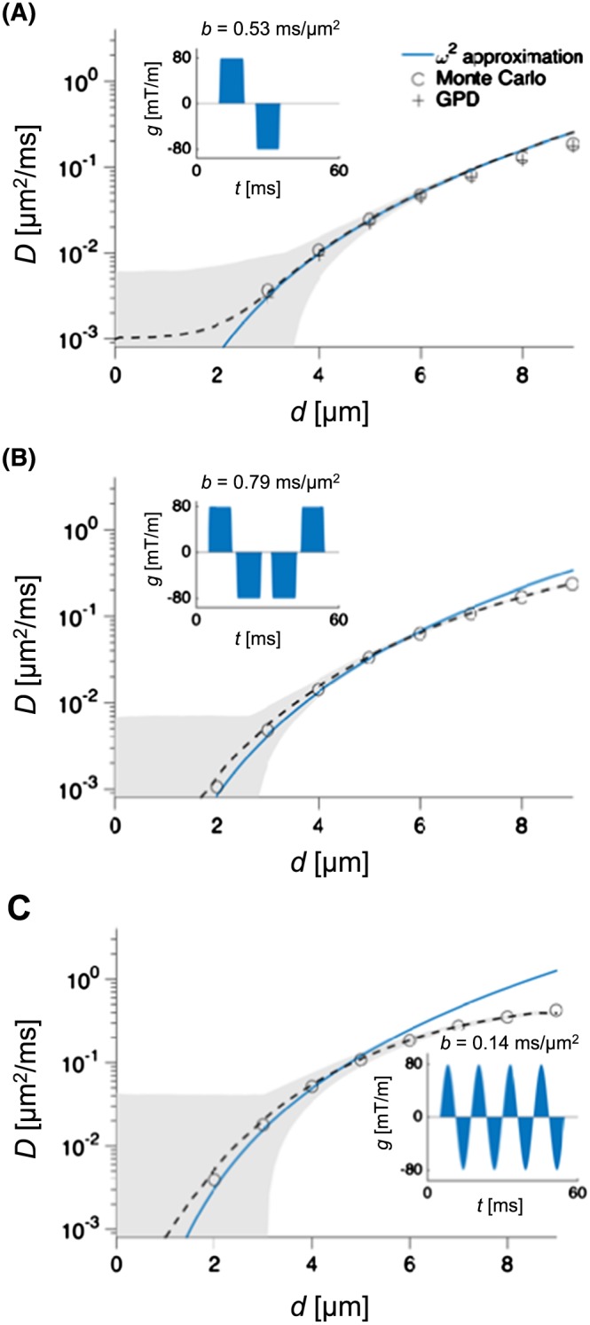
Low‐frequency approximation versus Monte Carlo results. The plots show the apparent radial diffusivity (D) predicted from the low‐frequency approximation (blue solid line), results from the Monte Carlo simulations (circles), and corresponding gradient waveforms (g(t)) and b‐values (inset). For the SDE case, the diffusivity predicted by the GPD approximation is also shown. The dashed line and the grey area show the mean and the 95% interval of the estimated diffusivities, assuming SNR = 1000. For small diameters (d), the low‐frequency approximation is in good agreement with the Monte Carlo simulations, whereas they start to diverge for larger diameters. In panel C, where the gradient waveform was a sine wave with f=80 Hz, the approximation agreed with the Monte Carlo simulations for d<5μm, as expected from Equation 21
Figure 3 shows the effect on the signal difference (ΔS) resulting from varying the frequency of a square‐wave oscillating gradient waveform, for cylinders where d=3.6μm. As the frequency increases, the b‐value decreases whereas D ⊥ increases. The net effect, however, is that ΔS is reduced for higher frequencies, illustrating that waveforms other than SDE lead to worse performance in terms of obtaining a minimal resolution limit for parallel cylinders. In the presence of orientation dispersion, however, the signal difference was maximised at a frequency of approximately 100 Hz. Note that here we assumed a slew rate of 200 mT/m/ms.
Figure 3.
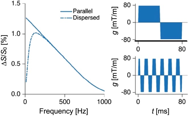
Impact of frequency on attenuation. The left panel shows ΔS, which is the signal difference between systems where d=3.6μm and d=0, for square‐wave oscillating gradients with varying frequency. Results are shown for both parallel and dispersed fibers. The two panels to the right shows the gradient waveforms that maximised ΔS for the parallel case (top) and the dispersed case (bottom)
Figure 4 shows a comparison of the resolution limit computed by our theoretical approach (Equations 34 and 40), and from the numerical approach described by Drobnjak et al.24 Investigations were performed under varying and SNR, assuming infinite slew rates. Panel A shows that numerical and analytical results were in excellent agreement for all gradient strengths and all SNR levels, for parallel cylinders. Panel B shows the results for fully dispersed cylinders. Here, the resolution limits depend on the number of oscillations m. Numerical and analytical results were well aligned except at low SNR levels, where our analytical approach underestimated the resolution limit. The discrepancies decreased at higher SNR, and for SNR=50 the match was excellent.
Figure 4.
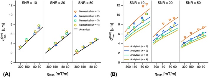
Resolution limit ( ) compared between analytical and numerical approaches. Panel A shows results for parallel cylinders under varying SNR levels, maximal gradient amplitudes ( ), and for a varying number of square‐wave oscillations (m) assuming infinite slew rates. The two approaches show excellent agreement. Panel B shows the corresponding result for the case with complete orientation dispersion. Resolution limits were higher than for the parallel case, as expected. The analytical approach underestimates the resolution limit for low SNR values, but the two approaches show good agreement for higher SNR levels. In all cases, the x‐axis was scaled according to
4.2. Optimisation
Figure 5 shows gradient waveforms optimised to minimise . In the case of parallel cylinders, the optimisation resulted in SDE waveforms, regardless of . This is not surprising, since SDE maximises η(Equation 30). In the case of fully dispersed cylinders, the optimal waveforms comprised a train of square pulses. For the case with stronger gradients, the waveforms became triangular, due to limitations in the available slew rate.
Figure 5.
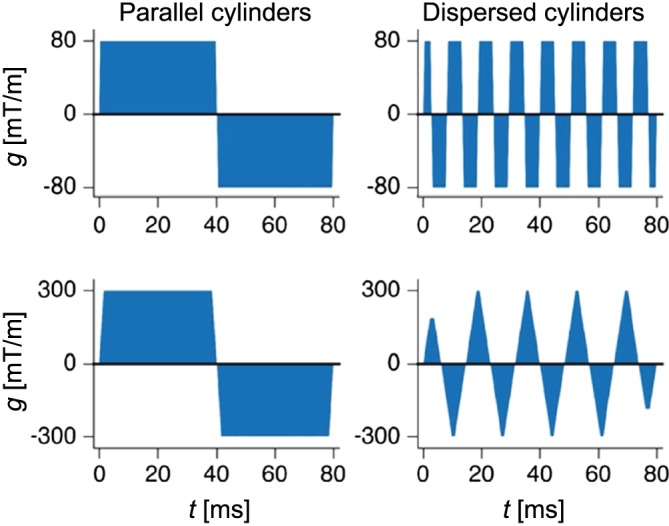
Waveforms optimised for best possible resolution. In the case of parallel cylinders, the optimisation resulted in SDE waveforms. For the dispersed case, waveforms included multiple gradient pulses. With a 80 mT/m system, a square‐wave oscillating waveform emerged. For the 300 mT/m system, the limited slew rate prevented the emergence of a square wave, and thus a triangular wave appeared instead
Table 1 shows the resolution limit in the cases of parallel and dispersed cylinders. The resolution limit was 20% higher in the presence of orientation dispersion for the 80 mT/m gradient system. For the 300 mT/m system, the corresponding number was 40%. For completeness, we also investigated the resolution limit for a preclinical system with 1000 mT/m gradients (slew rate 5000 T/m/s and T=30ms), and found it to be of the order of 1 μm.
Table 1.
Resolution limits ( ) for waveforms optimised so that ΔS=1%, with a waveform amplitude of and a duration of T=80 ms at field strength B 0=3T and T=50 ms at B 0=7T. The unit of the encoding strength b is ms/μm2
|
|
B 0 | b | b | |||
|---|---|---|---|---|---|---|
| 80 mT/m | 3T | 3.3 μm | 20 | 3.4 μm | 0.1 | |
| 300 mT/m | 3T | 1.7 μm | 260 | 2.6 μm | 1.4 | |
| 60 mT/m | 7T | 3.5 μm | 2.4 | 3.7 μm | 0.1 | |
| 80 mT/m | 7T | 3.0 μm | 4.5 | 3.2 μm | 0.1 |
In the intermediate case between coherence and full dispersion, the resolution limit depends on the specific level of orientation dispersion. For the level of dispersion recorded for the corpus callosum (FWHM = 34° , see Leergaard et al.73), we find for the 300 mT/m system, which is approximately 15–20% higher than the case for parallel fibres. In other words, even for an orientation dispersion as small as the one in the corpus callosum, otherwise known for its high orientation coherence, the resolution is degraded.
At 7T, the SNR is higher while the T 2 relaxation time is shorter (approximately 50 ms), thus requiring the use of shorter gradient pulses. Whether there is a benefit at 7T compared with 3T depends on the gradient system. If 80 mT/m is available at both 3T and 7T, the higher field strength has an advantage (Table 1).
4.3. Recovery
The ability to recover cylinder diameters from a simple experiment with two b‐values (0 and ) was assessed by numerical simulations. As shown in Figure 6 for a SDE‐like experiment in a system with parallell cylinders, diameters were correctly recovered above the resolution limit at . However, below this limit, cylinders of different sizes were indistinguishable.
Figure 6.
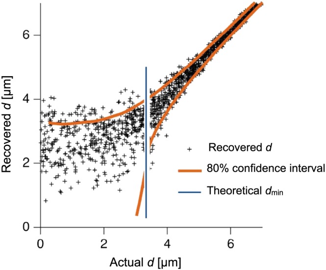
Recovery of cylinder diameters (d). Red lines show the 80% confidence interval. The resolution limit is shown as the blue vertical line, at m. The data represent a case with parallel cylinders and SDE encoding with δ=Δ=40ms
5. DISCUSSION
In this work, we assessed the minimal cylinder diameter that can be recovered from diffusion MRI of water within the cylinders. We label this diameter ‘the resolution limit’, in analogy with optical microscopy, where the diffraction limit defines the best optical resolution of the microscope. The theory presented herein allows the resolution limit to be assessed for arbitrary gradient waveforms, and also shows how to optimise the gradient waveform in order to minimise the resolution limit. In the very simple case of parallel cylinders, we demonstrated that the SDE experiment is preferred over any other waveform, which is in agreement with the findings of Drobnjak et al.,24 who used numerical simulations to compare SDE with ODE. Other studies have reported DDE to be beneficial for size estimation,34, 63 which stands in apparent contrast to our findings. However, those studies compare an optimised DDE with a suboptimal SDE, in the sense that the values of η(Equation 30) were not maximised for SDE and DDE separately (with T as the longest time common to the two sequences). Although DDE sequences are not intrinsically beneficial for size estimation, DDE has other unique applications, for example to study diffusion diffraction,74 water exchange,75, 76, 77, 78, 79 and intra‐voxel incoherent flow of blood.52 DDE is also useful for estimation of microscopic anisotropy,80, 81 although this is also possible with QTE, which may be experimentally advantageous compared with DDE.42, 82, 83, 84
The theory developed herein can be used to define three spatiotemporal regimes of the diffusion encoding. In the first regime, the diffusion is completely restricted and . In the second regime, the diffusion is partly restricted and , where f 0 is the maximal relevant frequency component of the encoding spectrum. In the third regime, the diffusion is weakly restricted and . The motional narrowing regime encompasses both the first and second regimes, whereas the third regime is a mixture of the motional narrowing and the free diffusion regimes described by Hurlimann et al.62 These regimes can be applied to simplify modelling of restricted diffusion. In the first regime, we can assume D ⊥=0, and in the second, D ⊥ can be reliably calculated using only V ω based on the low‐frequency approximation. In the third regime, knowledge of the full encoding spectrum is required to predict D ⊥, and thereby specific details such as the number of oscillations of the waveform become relevant.
According to our analysis, the analytically computed resolution limit is in perfect agreement with numerical results in the completely and partly restricted regimes (Figure 4). However, in the weakly restricted regime, the low‐frequency assumption does not hold. As a result, the analytically calculated resolution limit is underestimated, especially at a large number of oscillations. Nevertheless, even for these scenarios, the curves from the analytical and numerical approaches synchronously follow the same trend, determined by b V ω(Figure 4). Note that, in clinical scanners, gradient waveforms have little encoding power above 100 Hz, which yields d=4–5μm as the boundary between the partially and weakly restricted regimes.
The present analysis concerns diffusion in cylinders, and can be used to analyse axon diameter estimation by methods that model axons as straight cylinders.8, 20, 21 Our analysis suggests that gradient amplitudes in currently available clinical systems are insufficient to quantify the axon diameter accurately. This result is in agreement with Sepehrband et al.,85 who showed that the axon diameter estimated by such models depends on up to 1350 mT/m, which indicates that diameters probed by weaker gradients reflect the available amplitude rather than the underlying diameters. Moreover, in most of the white matter, axons do not run in straight and parallel courses, but rather in tortuous and non‐parallel configurations.27, 64 Even in a structure such as the corpus callosum, where axons are unusually coherent, there is substantial orientation dispersion.65, 66 In the presence of orientation dispersion, higher b‐values reduce the effective SNR, since the intra‐axonal water signal is attenuated proportional to the relative alignment of the axon to the direction of the diffusion encoding. Reducing the b‐value thus improves SNR, but if this is done by just reducing g, the resolution gets worse. A key result of the present study offers an alternative. Close to the resolution limit, the most important determinant of the signal attenuation is the integral of the squared gradient (b V ω). This entity can be kept constant, while b and V ω can be varied independently by the use of square‐wave oscillating gradients. In order to improve the SNR and thus improve the resolution, waveforms should, in the presence of dispersion, use more oscillations and hence lower b‐values than for the parallel case. This finding is in agreement with the results of Drobnjak et al.24 We also see that, with orientation dispersion, the relative benefit of using strong gradients to achieve high b‐values diminishes (Table 1).
We wish to highlight three limitations concerning the extrapolation of the present theoretical results to practical estimation of axon diameters in white matter. First, we investigate a simplified case where there is only intra‐axonal water. However, we believe the resolution limits reported herein to be applicable also to multi‐component systems, at least as lower limits, since adding complexity such as partial volume effects to the model will only make it more difficult to estimate the diameter accurately, not easier. The second limitation concerns the relationship between the axon diameter and the structure of the extra‐cellular space,47 which we neglected in the present analysis by considering the intra‐axonal component only. Including the extra‐cellular space in the model may, however, contribute with information on structural dimensions on its own.47, 86 Due to its weaker frequency dependence (|ω| versus ω 2), the resolution limit for estimating structural dimensions of the extracellular versus intra‐axonal space may differ, and, for low frequencies, effects of time‐dependent diffusion in the extra‐cellular space may dominate over those in the intra‐axonal space. Third and finally, the present analysis neglects exchange between water environments. However, exchange can probably be safely neglected, since our previous results have shown exchange times in white matter that are of the order of seconds or longer,78 which is much longer than the time‐scales during which effects of restricted diffusion can be observed.
Finally, note that the diffraction limit in optical microscopy, introduced in 1873, was recently broken.87 It took 135 years. Perhaps breaking the resolution limit in diffusion MRI can be done a little faster?
Acknowledgments
The authors acknowledge the NIH grants R01MH074794, R01MH092862, P41RR013218, P41EB015902, and the Swedish Research Council (VR) grants 2012‐3682, 2011‐5176, 2014‐3910, the CR Award (MN15), and the Swedish Foundation for Strategic Research (SSF) grant AM13‐0090.
Appendix 1. Gaussian phase dispersion (SDE case)
1.1.
We can utilize the GPD approximation to express k(α,β) as in Equation 7 of Nilsson et al.,8
| (A1) |
with a m defined by , so that are the roots of the derivative of the Bessel function of the first kind and order.
A.2. Slew rate
The maximal frequency content of a gradient waveform is limited by the maximal slew rate . We can express the effective gradient g(t) in terms of a convolution between an ideal gradient and a kernel K(t) that depends on the slew rate, according to
| (A2) |
The width of the kernel K(f) will thus determine the maximal frequency content of q(f). The lower the slew rate, the wider K(t) becomes and the narrower the support in K(f). The slew performance of the gradient system thus limits the maximal frequencies that can occur with reasonable energy in q(f). For simplicity, we express K with a Gaussian:
| (A3) |
where σ K(t) and σ K(f) refer to standard deviations in the time and frequency domains, respectively. Hence, |K(f)|2 is approximately zero for , which for and mT/m/ms equates to 1500 Hz.
A.3. Diffusion encoding spectra
For planar, cylindrical and spherical geometries, the frequency‐dependent apparent diffusion coefficient is the weighted sum of negative Lorentzians:57
| (A4) |
where, for a cylinder,
| (A5) |
Here, μ i are the roots to , and (·) is the Bessel function of the first kind and order.57 Let
| (A6) |
so that
| (A7) |
and
| (A8) |
The Lorenzian function above has a Taylor expansion according to
| (A9) |
At this point in time, we are only interested in the first two terms, i.e.
| (A10) |
Hence,
| (A11) |
where
| (A12) |
and
| (A13) |
according to Equation (33) in Wang et al.55 This derivation results in a compact low‐frequency approximation of the encoding spectrum in a cylinder,
| (A14) |
This result is also found in Eq. D.4 of Burcaw et al.47
M Nilsson, S Lasič, I Drobnjak, D Topgaard, C‐F Westin. Resolution limit of cylinder diameter estimation by diffusion MRI: The impact of gradient waveform and orientation dispersion, NMR Biomed. 2017;30:e3711 https://doi.org/10.1002/nbm.3711
References
- 1. Hursh J. Conduction velocity and diameter of nerve fibers. Am J Physiology. 1939;127:131–139. [Google Scholar]
- 2. Rushton WAH. A theory of the effects of fibre size in medullated nerve. J Physiol. 1951;115:101–122. [DOI] [PMC free article] [PubMed] [Google Scholar]
- 3. Waxman SG, Bennett MV. Relative conduction velocities of small myelinated and non‐myelinated fibres in the central nervous system. Nature. 1972;238:217–219. [DOI] [PubMed] [Google Scholar]
- 4. Edgar J, Griffiths I. White matter structure: A microscopists view Diffusion MRI: From Quantitative Measurement to In‐vivo Neuroanatomy: Academic Press; 2009:75–103. [Google Scholar]
- 5. Perge JA, Koch K, Miller R, Sterling P, Balasubramanian V. How the optic nerve allocates space, energy capacity, and information. J Neurosci. 2009;29:7917–7928. [DOI] [PMC free article] [PubMed] [Google Scholar]
- 6. Innocenti GM, Caminiti R, Aboitiz F. Comments on the paper by Horowitz et al. (2014). Brain Struct Func. 2015:1789–1790. [DOI] [PubMed] [Google Scholar]
- 7. Packer KJ, Rees C. Pulsed NMR studies of restricted diffusion. I. Droplet size distributions in emulsions. J Colloid Interface Sci. 1972;40:206–218. [Google Scholar]
- 8. Nilsson M, Westen D, Ståhlberg F, Sundgren PC, Lätt J. The role of tissue microstructure and water exchange in biophysical modelling of diffusion in white matter. Magn Reson Mater Phy. 2013;26:345–370. [DOI] [PMC free article] [PubMed] [Google Scholar]
- 9. Assaf Y, Cohen Y. Assignment of the water slow‐diffusing component in the central nervous system using q‐space diffusion MRS: implications for fiber tract imaging. Magn Reson Med. 2000;43:191–199. [DOI] [PubMed] [Google Scholar]
- 10. Assaf Y, Blumenfeld‐Katzir T, Yovel Y, Basser PJ. AxCaliber: a method for measuring axon diameter distribution from diffusion MRI. Magn Reson Med. 2008;59:1347–1354. [DOI] [PMC free article] [PubMed] [Google Scholar]
- 11. Benjamini D, Komlosh ME, Holtzclaw LA, Nevo U, Basser PJ. White matter microstructure from nonparametric axon diameter distribution mapping. NeuroImage. 2016;135:333–344. [DOI] [PMC free article] [PubMed] [Google Scholar]
- 12. Setsompop K, Kimmlingen R, Eberlein E, et al. Pushing the limits of in vivo diffusion MRI for the Human Connectome Project. NeuroImage. 2013;80:220–233. [DOI] [PMC free article] [PubMed] [Google Scholar]
- 13. Cohen Y, Assaf Y. High b‐value q‐space analyzed diffusion‐weighted MRS and MRI in neuronal tissues – a technical review. NMR Biomed. 2002;15:516–542. [DOI] [PubMed] [Google Scholar]
- 14. Lätt J, Nilsson M, Malmborg C, et al. Accuracy of q‐space related parameters in MRI: simulations and phantom measurements. IEEE Trans Med Imag. 2007;26:1437–1447. [DOI] [PubMed] [Google Scholar]
- 15. Callaghan P, MacGowan D, Packer K, Zelaya F. High‐resolution q‐space imaging in porous structures. J Magn Reson. 1990;90:177–182. [Google Scholar]
- 16. Ong HH, Wright AC, Wehrli SL, et al. Indirect measurement of regional axon diameter in excised mouse spinal cord with q‐space imaging: Simulation and experimental studies. NeuroImage. 2008;40:1619–1632. [DOI] [PMC free article] [PubMed] [Google Scholar]
- 17. Abbe E. Beitrage zur theorie des mikroskops und der mikroskopischen wahrnehmung. Archiv fur mikroskopische Anatomie. 1873;9:413–418. [Google Scholar]
- 18. Goodman JW. Introduction to Fourier Optics. Greenwood Village: Roberts and Company Publishers; 2005. [Google Scholar]
- 19. Aboitiz F, Scheibel AB, Fisher RS, Zaidel E. Fiber composition of the human corpus callosum. Brain Res. 1992;598:143–153. [DOI] [PubMed] [Google Scholar]
- 20. Assaf Y, Freidlin RZ, Rohde GK, Basser PJ. New modeling and experimental framework to characterize hindered and restricted water diffusion in brain white matter. Magn Reson Med. 2004;52:965–978. [DOI] [PubMed] [Google Scholar]
- 21. Alexander DC, Hubbard PL, Hall MG, et al. Orientationally invariant indices of axon diameter and density from diffusion MRI. NeuroImage. 2010;52:1374–1389. [DOI] [PubMed] [Google Scholar]
- 22. Dyrby TB, Søgaard LV, Hall MG, Ptito M, Alexander DC. Contrast and stability of the axon diameter index from microstructure imaging with diffusion MRI. Magn Reson Med. 2013;70:711–721. [DOI] [PMC free article] [PubMed] [Google Scholar]
- 23. Nilsson M, Alexander DC. Investigating tissue microstructure using diffusion MRI: How does the resolution limit of the axon diameter relate to the maximal gradient strength?. Proc Intl Soc Mag Reson Med. 2012;20:3567. [Google Scholar]
- 24. Drobnjak I, Zhang H, Ianuş A, Kaden E, Alexander DC. PGSE, OGSE, and sensitivity to axon diameter in diffusion MRI: Insight from a simulation study. Magn Reson Med. 2016;75:688–700. [DOI] [PMC free article] [PubMed] [Google Scholar]
- 25. Zhang H, Hubbard PL, Parker GJM, Alexander DC. Axon diameter mapping in the presence of orientation dispersion with diffusion MRI. NeuroImage. 2011;56:1301–1315. [DOI] [PubMed] [Google Scholar]
- 26. Zhang H, Schneider T, Wheeler‐Kingshott CA, Alexander DC. NODDI: practical in vivo neurite orientation dispersion and density imaging of the human brain. NeuroImage. 2012;61:1000–1016. [DOI] [PubMed] [Google Scholar]
- 27. Nilsson M, Lätt J, Ståhlberg F, Westen D, Hagslätt H. The importance of axonal undulation in diffusion MR measurements: A Monte Carlo simulation study. NMR Biomed. 2012;25:795–805. [DOI] [PubMed] [Google Scholar]
- 28. Stejskal EO, Tanner JE. Spin diffusion measurements: Spin echoes in the presence of a time‐dependent field gradient. J Chem Phys. 1965;42:288–292. [Google Scholar]
- 29. Shemesh N, Jespersen SN, Alexander DC, et al. Conventions and nomenclature for double diffusion encoding NMR and MRI. Magn Reson Med. 2016;75:82–87. [DOI] [PubMed] [Google Scholar]
- 30. Cory DG, Garriway AN, Miller JB. Applications of spin transport as a probe of local geometry. Polym Prepr. 1990;31:149–150. [Google Scholar]
- 31. Mitra PP. Multiple wave‐vector extensions of the NMR pulsed‐field‐gradient spin‐echo diffusion measurement. Phys Rev B. 1995;51:15074. [DOI] [PubMed] [Google Scholar]
- 32. Koch MA, Finsterbusch J. Towards compartment size estimation in vivo based on double wave vector diffusion weighting. NMR in Biomedicine. 2011;24(10):1422–1432. [DOI] [PubMed] [Google Scholar]
- 33. Komlosh ME, Özarslan E, Lizak MJ, et al. Mapping average axon diameters in porcine spinal cord white matter and rat corpus callosum using d‐PFG MRI. NeuroImage. 2013;78:210–216. [DOI] [PMC free article] [PubMed] [Google Scholar]
- 34. Benjamini D, Komlosh ME, Basser PJ, Nevo U. Nonparametric pore size distribution using d‐PFG: comparison to s‐PFG and migration to MRI. J Magn Reson. 2014;246:36–45. [DOI] [PMC free article] [PubMed] [Google Scholar]
- 35. Gross B, Kosfeld R. Anwendung der spin‐echo‐methode der messung der selbstdiffusion. Messtechnik. 1969;77:171–177. [Google Scholar]
- 36. Schachter M, Does MD, Anderson AW, Gore JC. Measurements of restricted diffusion using an oscillating gradient spin‐echo sequence. J Magn Reson. 2000;147:232–237. [DOI] [PubMed] [Google Scholar]
- 37. Callaghan PT, Stepisnik J. Frequency‐domain analysis of spin motion using modulated‐gradient NMR. J Magn Reson, Ser A. 1995;117:118–122. [Google Scholar]
- 38. Lasič S, Aslund I, Topgaard D. Spectral characterization of diffusion with chemical shift resolution: Highly concentrated water‐in‐oil emulsion. J Magn Reson. 2009;199:166–172. [DOI] [PubMed] [Google Scholar]
- 39. Shemesh N, Álvarez GA, Frydman L. Size distribution imaging by non‐uniform oscillating‐gradient spin echo (nogse) MRI. PloS One. 2015;10:e0133201. [DOI] [PMC free article] [PubMed] [Google Scholar]
- 40. Drobnjak I, Siow B, Alexander DC. Optimizing gradient waveforms for microstructure sensitivity in diffusion‐weighted MR. J Magn Reson. 2010;206:41–51. [DOI] [PubMed] [Google Scholar]
- 41. Eriksson S, Lasiċ S, Topgaard D. Isotropic diffusion weighting in PGSE NMR by magic‐angle spinning of the q‐vector. J Magn Reson. 2012;226:13–18. [DOI] [PubMed] [Google Scholar]
- 42. Westin CF, Knutsson H, Pasternak O, et al. Q‐space trajectory imaging for multidimensional diffusion MRI of the human brain. NeuroImage. 2016;135:345–362. [DOI] [PMC free article] [PubMed] [Google Scholar]
- 43. Sotiropoulos SN, Jbabdi S, Xu J, et al. Advances in diffusion MRI acquisition and processing in the Human Connectome Project. NeuroImage. 2013;80:125–143. [DOI] [PMC free article] [PubMed] [Google Scholar]
- 44. Ronen I, Budde M, Ercan E, Annese J, Techawiboonwong A, Webb A. Microstructural organization of axons in the human corpus callosum quantified by diffusion‐weighted magnetic resonance spectroscopy of N‐acetylaspartate and post‐mortem histology. Brain Structure and Function. 2014;219(5):1773–1785. [DOI] [PubMed] [Google Scholar]
- 45. Novikov DS, Jensen JH, Helpern JA, Fieremans E. Revealing mesoscopic structural universality with diffusion. Proc Natl Acad Sci USA. 2014;111:5088–5093. [DOI] [PMC free article] [PubMed] [Google Scholar]
- 46. Xu J, Li H, Harkins KD, et al. Mapping mean axon diameter and axonal volume fraction by MRI using temporal diffusion spectroscopy. NeuroImage. 2014;103C:10–19. [DOI] [PMC free article] [PubMed] [Google Scholar]
- 47. Burcaw LM, Fieremans E, Novikov DS. Mesoscopic structure of neuronal tracts from time‐dependent diffusion. NeuroImage. 2015;114:18–37. [DOI] [PMC free article] [PubMed] [Google Scholar]
- 48. Veraart J, Rajan J, Peeters RR, Leemans A, Sunaert S, Sijbers J. Comprehensive framework for accurate diffusion MRI parameter estimation. Magnetic Resonance in Medicine. 2013;70(4):972–984. [DOI] [PubMed] [Google Scholar]
- 49. Park MY, Byun JY. Understanding the mathematics involved in calculating apparent diffusion coefficient maps. Amer J Roentgenol. 2012;199:W784. [DOI] [PubMed] [Google Scholar]
- 50. Behrens TEJ, Woolrich MW, Jenkinson M, et al. Characterization and propagation of uncertainty in diffusion‐weighted MR imaging. Magn Reson Med. 2003;50:1077–1088. [DOI] [PubMed] [Google Scholar]
- 51. Nilsson M, Szczepankiewicz F, Westen D, Hansson O. Extrapolation‐based references improve motion and eddy‐current correction of high b‐value DWI data: Application in Parkinsons disease dementia. PloS One. 2015;10:e0141825. [DOI] [PMC free article] [PubMed] [Google Scholar]
- 52. Ahlgren A, Knutsson L, Wirestam R, et al. Quantification of microcirculatory parameters by joint analysis of flow‐compensated and non‐flow‐compensated intravoxel incoherent motion (IVIM) data. NMR Biomed. 2016;29:640–649. [DOI] [PMC free article] [PubMed] [Google Scholar]
- 53. Murday J, Cotts R. Self‐diffusion coefficient of liquid lithium. J Chem Phys. 1968;48:4938–4945. [Google Scholar]
- 54. Neuman CH. Spin echo of spins diffusing in a bounded medium. J Chem Phys. 1974;60:4508–4511. [Google Scholar]
- 55. Wang L, Caprihan A, Fukushima E. The narrow‐pulse criterion for pulsed‐gradient spin‐echo diffusion measurements. J Magn Reson, Ser A. 1995;117:209–219. [Google Scholar]
- 56. Aslund I, Topgaard D. Determination of the self‐diffusion coefficient of intracellular water using PGSE NMR with variable gradient pulse length. J Magn Reson. 2009;201:250–254. [DOI] [PubMed] [Google Scholar]
- 57. Stepisnik J. Time‐dependent self‐diffusion by NMR spin‐echo. Physica B. 1993;183:343–350. [Google Scholar]
- 58. Stepisnik J, Lasič S, Mohoric A, Sersa I, Sepe A. Spectral characterization of diffusion in porous media by the modulated gradient spin echo with CPMG sequence. J Magn Reson. 2006;182:195–199. [DOI] [PubMed] [Google Scholar]
- 59. Grebenkov DS. NMR survey of reflected Brownian motion. Rev Mod Phys. 2007;79:1077–1137. [Google Scholar]
- 60. Cates G, Schaefer S, Happer W. Relaxation of spins due to field inhomogeneities in gaseous samples at low magnetic fields and low pressures. Phys Rev A. 1988;37:2877–2885. [DOI] [PubMed] [Google Scholar]
- 61. Stoller S, Happer W, Dyson F. Transverse spin relaxation in inhomogeneous magnetic fields. Phys Rev A. 1991;44:7459–7477. [DOI] [PubMed] [Google Scholar]
- 62. Hurlimann M, Helmer K, Deswiet T, Sen P. Spin echoes in a constant gradient and in the presence of simple restriction. J Magn Reson, Ser A. 1995;113:260–264. [Google Scholar]
- 63. Katz Y, Nevo U. Quantification of pore size distribution using diffusion NMR: experimental design and physical insights. J Chem Phys. 2014;140:164201. [DOI] [PubMed] [Google Scholar]
- 64. Jeurissen B, Leemans A, Tournier JD, Jones DK, Sijbers J. Investigating the prevalence of complex fiber configurations in white matter tissue with diffusion magnetic resonance imaging. Hum Brain Mapp. 2013;34:2747–2766. [DOI] [PMC free article] [PubMed] [Google Scholar]
- 65. Budde MD, Frank JA. Examining brain microstructure using structure tensor analysis of histological sections. NeuroImage. 2012;63:1–10. [DOI] [PubMed] [Google Scholar]
- 66. Ronen I, Budde M, Ercan E, Annese J, Techawiboonwong A, Webb A. Microstructural organization of axons in the human corpus callosum quantified by diffusion‐weighted magnetic resonance spectroscopy of N‐acetylaspartate and post‐mortem histology. Brain Struct Func. 2014;219:1773–1785. [DOI] [PubMed] [Google Scholar]
- 67. Callaghan PT, Jolley KW, Lelievre J. Diffusion of water in the endosperm tissue of wheat grains as studied by pulsed field gradient nuclear magnetic resonance. Biophys J. 1979;28:133–141. [DOI] [PMC free article] [PubMed] [Google Scholar]
- 68. Callaghan PT, Söderman O. Examination of the lamellar phase of aerosol OT/water using pulsed field gradient nuclear magnetic resonance. J Phys Chem. 1983;87:1737–1744. [Google Scholar]
- 69. Eriksson S, Lasič S, Nilsson M, Westin CF, Topgaard D. NMR diffusion‐encoding with axial symmetry and variable anisotropy: Distinguishing between prolate and oblate microscopic diffusion tensors with unknown orientation distribution. J Chem Phys. 2015;142:104201. [DOI] [PMC free article] [PubMed] [Google Scholar]
- 70. Carr HY, Purcell EM. Effects of diffusion on free precession in nuclear magnetic resonance experiments. Phys Rev. 1954;94:630–638. [Google Scholar]
- 71. Nilsson M, Alerstam E, Wirestam R, Ståhlberg F, Brockstedt S, Lätt J. Evaluating the accuracy and precision of a two‐compartment Kärger model using Monte Carlo simulations. J Magn Reson. 2010;206:59–67. [DOI] [PubMed] [Google Scholar]
- 72. Drobnjak I, Zhang H, Hall MG, Alexander DC. The matrix formalism for generalised gradients with time‐varying orientation in diffusion NMR. J Magn Reson. 2011;210:151–157. [DOI] [PubMed] [Google Scholar]
- 73. Leergaard TB, White NS, De Crespigny A, et al. Quantitative histological validation of diffusion MRI fiber orientation distributions in the rat brain. PLoS One. 2010;e8595:5. [DOI] [PMC free article] [PubMed] [Google Scholar]
- 74. Shemesh N, Ozarslan E, Adiri T, Basser PJ, Cohen Y. Noninvasive bipolar double‐pulsed‐field‐gradient NMR reveals signatures for pore size and shape in polydisperse, randomly oriented, inhomogeneous porous media. J Chem Phys. 2010;133:044705. [DOI] [PMC free article] [PubMed] [Google Scholar]
- 75. Callaghan PT, Furó I. Diffusion–diffusion correlation and exchange as a signature for local order and dynamics. J Chem Phys. 2004;120:4032–4038. [DOI] [PubMed] [Google Scholar]
- 76. Åslund I, Nowacka A, Nilsson M, Topgaard D. Filter‐exchange PGSE NMR determination of cell membrane permeability. J Magn Reson. 2009;200:291–295. [DOI] [PubMed] [Google Scholar]
- 77. Lasič S, Nilsson M, Lätt J, Ståhlberg F, Topgaard D. Apparent exchange rate mapping with diffusion MRI. Magn Reson Med. 2011;66:356–365. [DOI] [PubMed] [Google Scholar]
- 78. Nilsson M, Lätt J, Westen D, et al. Noninvasive mapping of water diffusional exchange in the human brain using filter‐exchange imaging. Magn Reson Med. 2013;69:1572–1580. [DOI] [PubMed] [Google Scholar]
- 79. Schilling F, Ros S, Hu DE, et al. MRI measurements of reporter‐mediated increases in transmembrane water exchange enable detection of a gene reporter. Nat Biotechnol. 2016. doi: 10.1038/nbt.3714. [DOI] [PMC free article] [PubMed] [Google Scholar]
- 80. Özarslan E, Basser PJ. Microscopic anisotropy revealed by NMR double pulsed field gradient experiments with arbitrary timing parameters. J Chem Phys. 2008;128:154511. [DOI] [PMC free article] [PubMed] [Google Scholar]
- 81. Jespersen SN, Lundell H, Sønderby CK, Dyrby TB. Orientationally invariant metrics of apparent compartment eccentricity from double pulsed field gradient diffusion experiments. NMR Biomed. 2013;26:1647–1662. [DOI] [PubMed] [Google Scholar]
- 82. Lasič S, Szczepankiewicz F, Eriksson S, Nilsson M, Topgaard D. Microanisotropy imaging: quantification of microscopic diffusion anisotropy and orientational order parameter by diffusion MRI with magic‐angle spinning of the q‐vector. Frontiers in Physics. 2014;2:11. [Google Scholar]
- 83. Szczepankiewicz F, Lasiċ S, Westen D, et al. Quantification of microscopic diffusion anisotropy disentangles effects of orientation dispersion from microstructure: Applications in healthy volunteers and in brain tumors. Neuroimage. 2015;104:241–252. [DOI] [PMC free article] [PubMed] [Google Scholar]
- 84. Szczepankiewicz F, Westen D, Englund E, et al. The link between diffusion MRI and tumor heterogeneity: Mapping cell eccentricity and density by diffusional variance decomposition (DIVIDE). NeuroImage. 2016;142:522–532. [DOI] [PMC free article] [PubMed] [Google Scholar]
- 85. Sepehrband F, Alexander DC, Kurniawan ND, Reutens DC, Yang Z. Towards higher sensitivity and stability of axon diameter estimation with diffusion‐weighted MRI. NMR Biomed. 2016;29:293–308. [DOI] [PMC free article] [PubMed] [Google Scholar]
- 86. Fieremans E, Burcaw LM, Lee HH, Lemberskiy G, Veraart J, Novikov DS. In vivo observation and biophysical interpretation of time‐dependent diffusion in human white matter. NeuroImage. 2016;129:414–427. [DOI] [PMC free article] [PubMed] [Google Scholar]
- 87. Zhang X, Liu Z. Superlenses to overcome the diffraction limit. Nat Mater. 2008;7:435–441. [DOI] [PubMed] [Google Scholar]