Zero- to low-field MRI with averaging of concomitant gradient fields

Abstract

Magnetic resonance imaging (MRI) encounters fundamental limits in circumstances in which the static magnetic field is not sufficiently strong to truncate unwanted, so-called concomitant components of the gradient field. This limitation affects the attainable optimal image fidelity and resolution most prominently in low-field imaging. In this article, we introduce the use of pulsed magnetic-field averaging toward relaxing these constraints. It is found that the image of an object can be retrieved by pulsed low fields in the presence of the full spatial variation of the imaging encoding gradient field even in the absence of the typical uniform high-field time-independent contribution. In addition, error-compensation schemes can be introduced through the application of symmetrized pulse sequences. Such schemes substantially mitigate artifacts related to evolution in strong magnetic-field gradients, magnetic fields that vary in direction and orientation, and imperfections of the applied field pulses.

Over the past three decades, magnetic resonance imaging (MRI) has proven to be remarkably successful for producing images of samples ranging from human subjects (1) to single cells (2). The seminal concept of “image formation by induced local interaction” (3) is based on rendering the NMR frequency dependent on spatial coordinates, which is generally accomplished by supplementing a strong homogeneous magnetic field (B₀) with a secondary magnetic field (the gradient field) of known spatial distribution. The additional field serves to modulate the local amplitude of the total field. As a consequence, there is a (typically linear) relationship between the strength of the interaction (reflected in the resonance frequency) and the spatial location, where the interaction takes place, thereby affording an encoding of the spatial information into NMR spectral frequencies and phases.

To produce a purely amplitude-modulated magnetic field, it is well known that gradient field components perpendicular to B₀ must be suppressed. Such components are of necessity present in a field with amplitude that varies spatially. To satisfy Maxwell's equations, every physical magnetic field in free space must be curl- and divergence-free so that it cannot vary exclusively in amplitude and must therefore vary also in direction, implying that the magnetic-field quantization axis is not constant across the sample. Traditionally, the perpendicular components [in the context of MRI usually referred to as “concomitant fields” (4)] are suppressed by restricting the gradient fields to absolute values much smaller than B₀, which ensures that the undesired components of the gradient field are “nonsecular” and that they can effectively be truncated and correspondingly ignored.

There are cases, however, in which supplementing the gradient field with a static “truncating field” is not favorable (or even impossible). One such situation is “ex situ NMR,” in which the sample is not, as is usual, immersed in a magnet but placed outside in a region where the field varies in magnitude and also possibly in direction. Another prominent example is low-field MRI, in which a low magnetic field [typically on the order of 1 μT (5, 6) to 1 mT (7, 8)] serves as a truncating field, the extreme limit of which is zero-field NMR and MRI. Inherent advantages such as cost or the avoidance of high-field artifacts (e.g., ghosting due to susceptibility broadening or chemical shift) and skin-depth penetration through metal have made this area of “ultralow field” particularly attractive. However, the maximum allowed gradient field strength (typically at least 5–10 times less than B₀) is a restriction that imposes a limit on the ultimately attainable resolution.

Complementing an early attempt (9), we investigate a scheme aimed at reconstructing images in very low magnetic fields by averaging away the effects of the concomitant field gradient components. Our approach is based on the use of trains of magneticfield pulses. Spatial encoding is achieved by periodically allowing the system to evolve in the field created by a gradient coil. Here, however, the evolution takes place in the absence of a high truncating field. A first numerical example using the field caused by a Golay (or saddle) coil (10) is shown in Fig. 1: if we take as a starting point the spin distribution obtained at high field, it is possible to reconstruct this image by interleaving pulses of uniform and gradient fields. As will be shown next, the scheme leads to an effective truncation of the encoding gradient. This truncation, however, is independent of the relative field strengths but rather results from the cycle period in the (field) pulse train.

Fig. 1.

Reconstruction of an image encoded in a pure gradient field. (Inset) Two-dimensional image of a brain obtained in a commercial MRI system at 3 T. Each dimension has a total of 256 points, and the number of spins at each site was assumed strictly proportional to the intensity. Interpreted as a spin map, the grid was then stored in the computer memory and was taken as the starting point for a numerical simulation. Shown in the main figure is a numerical reconstruction of the brain image in the absence of a uniform static magnetic field. The used field-pulse scheme is explained in the text (see also Fig. 2 A). The dc-field pulses had an amplitude of 3 G(1G = 0.1 mT), and within each train the interpulse interval was 0.5 ms. The gradient amplitude was equal to 0.03 G/cm (130 Hz/cm). The number of points acquired was 1,024 in each of the 512 projections recorded, and data treatment was standard. The (elliptical) halo around the brain is an effect caused by projection/reconstruction (see Fig. 3).

Let us start by considering the magnetic field created by a saddle coil. This coil is usually designed in a way to create (in the presence of a strong B₀) a linear gradient ∂B_z/∂x = g = constant across the sample region. The field at each point (x, z) is then

[1]

as readily derived from the condition that 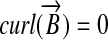. The Hamiltonian of a single spin in the presence of this magnetic field can be written as

[2]

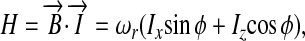
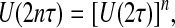
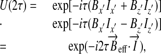
where 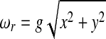and tanϕ = z/x; for simplicity, we have assumed a unitary magnetogyric ratio. Eq. 2 implies that the resonance frequency only depends on the radial distance to the center of the array, i.e., the frequency spectrum only contains radial but no angular information. A first scheme aimed at overcoming this limitation is shown in Fig. 2A: a train of (short) spatially uniform dc-field pulses B_dc is applied during spin evolution along the direction x̂′; the duration of these pulses is chosen so as to induce π rotations. The gradient field is turned on in the intervals τ between these pulses. If the acquisition is performed stroboscopically after every other pulse, the evolution operator U evaluated at the nth cycle satisfies the relation

[3]

where U(2τ) = exp(–iHτ)exp(–iπ I_x′)exp(–iHτ)exp(–iπ I_x′). Explicitly rewriting the Hamiltonian and using the Magnus expansion, we get

[4]

with (11, 12) , showing that when the interpulse spacing is sufficiently short, the effective field points in the direction x̂′ of the pulses. If we denote by θ the angle between this direction and the x axis, a simple geometrical consideration leads to B_x′ = g(zcosθ + xsinθ). Thus, the effective field magnitude is given by

[5]

where , , and γ = (π /2) – θ. This result implies that when the train of uniform dc-field pulses is applied along a direction x̂′ = (cosθ, sinθ), the effective field (and, thereby, the projection axis of the image) points along a direction . Thus, this method is equivalent to projection/reconstruction with the exception that, in the present case, the change in the resulting gradient direction is accomplished by a change in the direction of the effective field (see Fig. 2) (13, 14).§

Fig. 2.

Pulse sequence and image reconstruction scheme. (A) The system is initially prepolarized along the y axis (perpendicular to the paper surface). A train of uniform dc-field π pulses along a direction x̂′ making an angle θ with the x axis manipulates further evolution in the gradient field. The pulse repetition rate has to be fast compared to the maximum local Larmor frequency in the gradient field. Acquisition (Acq) is performed stroboscopically in between pulses. Different acquisition schemes are possible. The one indicated above the pulses (black) symmetrizes the cycle, canceling out all odd terms in the average Hamiltonian expansion. The one below the pulse train (gray) is appropriate for a longer dead time of the detector (the first π pulse has been included for didactical reasons but is not necessary). (B) As the direction x̂′ of the dc-field pulses changes (Left), so do the direction of the effective field (always pointing in the direction of the pulses) and the direction x̂″ of the effective gradient (Right), here indicated by the angle γ. A series of image projections can then be obtained, leading to the full reconstruction of the spatial spin distribution.

Fig. 3 displays the results of numerical simulations for the case of a simplified phantom. In contrast to the case shown in Fig. 1, rather unfavorable conditions have been chosen here to highlight some of the scheme limitations. Spins are distributed on a Cartesian grid with 128 × 128 points, and their magnitudes have been assigned so as to reproduce the spin density of Fig. 3A. We have assumed that the spins were initially aligned along the y axis (normal to the figure plane) and that self-diffusion effects during the pulse train are negligible. Fig. 3C shows the image obtained after only 25 projections and a standard processing using projection/reconstruction (Fig. 3B). The figure correctly reproduces the spatial density of the spin system, but it is clear that some artifacts show up as the distance to the center increases. This effect is intrinsic to the method of projection/reconstruction, and in the present case, the problem becomes more acute because the correction terms in Eq. 4 are more important in this region of the sample. Incomplete averaging also leads to a sharp peak at the center (where the resonance frequency is actually zero) because the effective field develops a nonnegligible component along the y axis. Nonetheless, a considerable improvement is attained if the spin state is inspected at half the interpulse interval and not at the end (Fig. 3D), which is because the repeating unit during the system evolution becomes symmetric, and as a consequence, all odd terms of the Magnus expansion become zero (11).

Fig. 3.

Tensor field imaging. (A) Virtual spin distribution on a square surface from –5 to 5 cm with a 0.1-cm mesh. Circles have 0.5-cm radii and are 2 cm apart from each other. (B) Standard projection/reconstruction in the presence of a strong and homogeneous magnetic field. The concomitant gradient is truncated. Notice, however, the typical star-like behavior at large radii. (C) Tensor field imaging with acquisition at the end of the interpulse interval. The sharp peak at the center (zero frequency) is caused by imperfect averaging. (D) Same as described for C but with acquisition at half the interpulse interval (see Fig. 2A). For B–D, the gradient strength was 0.06 G/cm (250 Hz/cm), the dwell time was 1 ms, and the free induction decay had 256 points. Twenty-five equally spaced angles were used covering the range of 0–180. Pulses had an amplitude of 3 G.

Notice, finally, that remnant artifacts caused by projection/reconstruction vanish if, alternative to the straightforward approach discussed above, an adaptation of Fourier imaging is used. One possibility involves a 90° change of the pulsing direction at an intermediate variable point within the pulse train. In our case, a change in the direction of the effective gradient also creates a change in the direction of the effective field, which makes the situation a bit more complex. Such methods will be discussed in a forthcoming article, as well as the use of a minute constant uniform field in addition to the gradient to make the basic frequency nonzero. This situation will be relevant in the useful range of uniform and gradient fields of comparable magnitude.

In practice, imaging in the absence of a uniform magnetic field can be carried out in various ways. Magnetometry-based detection modalities seem today the most likely candidates for practical systems, because its frequency response is relatively flat and its sensitivity is considerably better at very low magnetic fields than inductive signal detection (5, 6). Nonetheless, some limitations are foreseeable: for example, detection at the center of the sample (where the magnetic field tends to zero) may be hampered, because in this region the 1/f noise becomes dominant and the detection sensitivity is reduced (15, 16). Another limitation is the finite recovery time of the detector, which in general precludes a very fast stroboscopic acquisition. This shortcoming can be overcome by altering the detection scheme such that the spin evolution is monitored indirectly point by point in a second time dimension.

An appealing advantage of the present approach is that the gradient amplitude (and, thereby, the image resolution) is constrained only by the experimental ability to pulse (and detect) sufficiently rapidly, which contrasts with the standard situation in which concomitant components of the gradient field can be made negligible only if they are kept much smaller than a uniform time-independent magnetic field. Interesting applications certainly can be envisioned, for example, in the area of magnetoencephalography (17–19) or, more generally, in situations in which the presence of a very low magnetic field is convenient or necessary. Progress in low-field magnetometry (20–22) is making the hardware implementations of these challenges a realistic possibility for the near future.

References

- 1.Chacko, A. K., Katzberg, R. W. & MacKay, A. (1991) MRI Atlas of Normal Anatomy (McGraw–Hill, New York).
- 2.Ciobanu, L., Webb, A. G. & Pennington, C. H. (2003) Prog. Nucl. Magn. Reson. Spectrosc. 42 69–93. [Google Scholar]
- 3.Lauterbur, P. C. (1973) Nature 242 190–191.16067082 [Google Scholar]
- 4.Norris, D. G. & Hutchinson, J. M. S. (1990) Magn. Reson. Imaging 8 33–37. [DOI] [PubMed] [Google Scholar]
- 5.McDermott, R., Trabesinger, A. H., Muck, M., Hahn, E. L., Pines, A. & Clarke, J. (2002) Science 295 2247–2249. [DOI] [PubMed] [Google Scholar]
- 6.McDermott, R., Lee, S.-K., ten Haken, B., Trabesinger, A. H., Pines, A. & Clarke, J. (2004) Proc. Natl. Acad. Sci. USA 101 7857–7861. [DOI] [PMC free article] [PubMed] [Google Scholar]
- 7.Wong-Foy, A., Saxena, S., Moulé, A. J., Bitter, H. M. L., Seeley, J. A., McDermott, R., Clarke, J. & Pines, A. (2002) J. Magn. Reson. 157 235–241. [DOI] [PubMed] [Google Scholar]
- 8.Tseng, C. H., Wong, G. P., Pomeroy, V. R., Mair, R. W., Hinton, D. P., Hoffmann, D., Stoner, R. E., Hersman, F. W., Cory, D. G. & Walsworth, R. L. (1998) Phys. Rev. Lett. 81 3785–3788. [DOI] [PubMed] [Google Scholar]
- 9.Agrawal, A. (2003) Ph.D. dissertation (Univ. of California, Berkeley).
- 10.Bottomley, P. A. (1981) J. Phys. E Sci. Instrum. 14 1081–1087. [Google Scholar]
- 11.Haeberlen, U. (1976) High-Resolution NMR in Solids: Selective Averaging (Academic, New York).
- 12.Ernst, R. R., Bodenhausen, G. & Wokaun, A. (1994) Principles of Nuclear Magnetic Resonance in One and Two Dimensions (Clarendon, Oxford).
- 13.Maas, W. E., Laukien, F. & Cory, D. G. (1993) J. Magn. Reson. A 103 115–117. [Google Scholar]
- 14.Cory, D. G., Laukien, F. H. & Maas, W. E. (1993) Chem. Phys. Lett. 212 487–492. [Google Scholar]
- 15.Clarke, J. & Hawkins, G. (1976) Phys. Rev. B 14 2826–2831. [Google Scholar]
- 16.Greenberg, Y. S. (1998) Rev. Mod. Phys. 70 175–222. [Google Scholar]
- 17.Hämäläinen, M., Hari, R., Ilmoniemi, R. J., Knuutila, J. & Lounasmaa, O. V. (1993) Rev. Mod. Phys. 65 413–497. [Google Scholar]
- 18.Volegov, P. L., Matlachov, A. N., Espy, M. A., George, J. S. & Kraus, R. H. (2004) Magn. Reson. Med. 52 467–470. [DOI] [PubMed] [Google Scholar]
- 19.Matlachov, A. N., Volegov, P. L., Espy, M. A., George, J. S. & Kraus, R. H. (2004) J. Magn. Reson. 270 1–7. [DOI] [PubMed] [Google Scholar]
- 20.Kominis, I. K., Kornack, T. W., Alfred, J. C. & Romalis, M. V. (2003) Nature 422 596–599. [DOI] [PubMed] [Google Scholar]
- 21.Pannetier, M., Fermon, C., Le Goff, G., Simola, J. & Kerr, E. (2004) Science 304 1648–1650. [DOI] [PubMed] [Google Scholar]
- 22.Yashchuk, V. V., Granwehr, J., Kimball, D. F., Rochester, S. M., Trabesinger, A. H., Urban, J. T., Budker, D. & Pines, A. (2004) Phys. Rev. Lett. 93 160801. [DOI] [PubMed] [Google Scholar]