Accelerated High-Dimensional MR Imaging with Sparse Sampling Using Low-Rank Tensors

Abstract

High-dimensional MR imaging often requires long data acquisition time, thereby limiting its practical applications. This paper presents a low-rank tensor based method for accelerated high-dimensional MR imaging using sparse sampling. This method represents high-dimensional images as low-rank tensors (or partially separable functions) and uses this mathematical structure for sparse sampling of the data space and for image reconstruction from highly undersampled data. More specifically, the proposed method acquires two datasets with complementary sampling patterns, one for subspace estimation and the other for image reconstruction; image reconstruction from highly undersampled data is accomplished by fitting the measured data with a sparsity constraint on the core tensor and a group sparsity constraint on the spatial coefficients jointly using the alternating direction method of multipliers. The usefulness of the proposed method is demonstrated in MRI applications; it may also have applications beyond MRI.

I. Introduction

High-dimensional MR imaging is desirable for many biomedical applications, such as dynamic cardiac imaging [1], multiparameter mapping [2], spectroscopic imaging [3], and diffusion imaging [4]. However, the number of encodings (data points) needed in conventional imaging methods grows exponentially with the dimensionality of the desired image function (known as the “curse of dimensionality”), which often leads to impractically long data acquisition times. To address this issue, a number of methods have been proposed in recent years for accelerated imaging with sparse sampling. Most notably, compressed sensing methods have successfully exploited the sparsity of images in various transform domains and achieved impressive results on sparse sampling. Since the early work [5]–[9], many extensions to sparse model-based accelerated imaging have been developed (e.g., design of random excitation schemes [10], [11], incorporation of group sparsity [12], partially known support [13]–[15], and parallel imaging [16]) and successfully used in practical applications [17]–[19]. Low-rank structures have also proved useful for sparse sampling. Existing low-rank based methods (e.g., [20]–[24]) have effectively exploited the spatiotemporal (or spatiospectral) correlation that exists in high-dimensional data. For example, early methods [20], [25], [26] utilize the low-rank structure of the Casorati matrix for accelerated imaging; these methods enforce an explicit subspace structure estimated from an auxiliary dataset. Low-rank matrix structure can also be enforced implicitly by using, for example, nuclear norm minimization [23], [27], [28]. More recent methods exploiting both low-rank structure and sparsity have been developed and shown to provide enhanced performance [23], [24], [29]. These methods have also been successfully applied to various MRI problems, e.g., real-time cardiac imaging [30], dynamic speech imaging [31], diffusion imaging [32], relaxometry [33] and spectroscopic imaging [34].

This paper extends the low-rank matrix-based approach by using low-rank tensors to capture data correlation in multiple dimensions, beyond just spatiotemporal or spatiospectral correlation. The use of tensor structures for accelerated imaging has been proposed in [35]–[39]. These methods either exploit sparsity of the high-order tensors (in the spirit of compressed sensing) or implicitly enforce low-rankness through penalty terms such as the nuclear norm. We propose a new method, called Low-Rank Tensor with “Explicit Subspace” (LRTES), that represents high-dimensional image functions using an explicit low-rank tensor model. Based on this model, we propose a data acquisition scheme characterized by acquisition of two complementary data sets: a navigator dataset for estimating the tensor subspace structure, and a sparse dataset for image reconstruction. The image reconstruction problem consists of two subproblems: 1) determining the basis functions of the tensor subspace from the navigator data, and 2) reconstructing high-dimensional data by fitting the measured data with the estimated subspace. We solve the first problem using SVD and the second problem using regularized least squares fitting with a sparsity constraint on the core tensor and a group sparsity constraint on the spatial coefficients jointly. The non-convex optimization problem associated with image reconstruction is solved using the alternating direction method of multipliers (ADMM).

The rest of this paper is organized as follows: Section II presents a summary of relevant mathematical results on low-rank tensors; Section III describes the proposed low-rank tensor based data acquisition with sparse sampling; Section IV discusses the proposed image reconstruction from highly undersampled data using low-rank tensors; Section V shows some representative results from several application examples of the proposed method, which is followed by the discussion and conclusion of the paper in Section VI.

II. Low-Rank Tensor Image Models

A. Notation

First-order tensors (i.e., vectors) are denoted by bold lowercase letters (e.g., a), second-order tensors (i.e., matrices) by bold capital letters (e.g., A), and tensors of order three or higher are denoted by Euler script letters (e.g., 𝒳). Scalars are denoted by lowercase italic letters (e.g., a). Indexed scalars, such as a_i, a_{i j}, and x_{i jk}, are used to represent the ith, (i, j)th, and (i, j,k)th element of vector a, matrix A, and third-order tensor 𝒳, respectively; vec(A) is a vectorized representation of (A) (i.e., the vector elements are taken from A column by column). We use A^T to denote the transpose of A, A^H the Hermitian transpose of A, and Ω^* the Hermitian adjoint of operator Ω. As in [40], we use ∘ to denote the vector outer product (or tensor product), and ⊗ to denote the Kronecker product. The following vector and matrix norms are also used: 1) ℓ₁ norm ${\Vert \mathbf{a}\Vert }_1\triangleq {\displaystyle \sum _i}\mid a_i\mid$; 2) Frobenius norm ${\Vert \mathbf{A}\Vert }_F\triangleq {({\displaystyle \sum _i}{\displaystyle \sum _j}{\mid a_{ij}\mid }^2)}^{1/2}$.

The mode-i matricization (also known as unfolding or flattening) of a tensor 𝒳 ∈ ℂ^{N₁×N₂×⋯×N_d} is defined as X_(n) ∈ ℂ^{N_i×(N_1⋯N_i−1N_i+1⋯N_d)}, arranging the data along the N_ith dimension to be the columns of X_(i). The opposite operation of tensor matricization is called the folding operation, which arranges the elements of the matrix X_(i) into the dth order tensor 𝒳.

Tensor multiplication is much more complex than matrix multiplication, and here we consider only the tensor i-mode product, defined as the multiplication (e.g., 𝒳 ×_iU) of a tensor 𝒳 with a matrix U ∈ ℂ^J×N_i in mode i. We have the elementwise presentation $y_{n_1\cdots n_{i-1}j{n}_{i+1}\cdots n_d}={\displaystyle \sum _{n_i=1}^{N_i}}{x}_{n_1\cdots n_{i-1}{n}_i{n}_{i+1}\cdots n_d}{u}_{j{n}_i}$, where 𝒴 = (𝒳 ×_iU) ∈ ℂ^{N₁×⋯N_i−1×J×N_i+1×⋯×N_d}. The i-mode product can also be presented in the matricized form: Y_(i) = UX_(i).

B. Low-rank tensor image models

Consider a d-dimensional image function ρ(x₁, x₂, ⋯ , x_d) that is support-limited and belongs to a certain Hilbert space. Such a function can often be “well” represented/approximated by lower-dimensional functions [20]. For example, we may express ρ(x₁, x₂, ⋯ , x_d) as

$$\rho (x_1,x_2,\cdots ,x_d)\approx \sum _{\ell =1}^L{g}_{\ell }^{(1)}(x_1)g_{\ell }^{(2)}(x_2)\cdots g_{\ell }^{(d)}(x_d)$$ (1)

where L is called the separation rank.¹ One extension of the model in (1) is

$$\rho (x_1,x_2,\cdots ,x_d)\approx \sum _{\ell =1}^L{g}_{\ell }^{(1)}({\mathbf{x}}_1)g_{\ell }^{(2)}({\mathbf{x}}_2)\cdots g_{\ell }^{(\widehat{d})}({\mathbf{x}}_{\widehat{d}}),$$ (2)

where {x₁,x₂, ⋯ ,x_d̂} represents d̂ groups of “separable” variables from {x₁, x₂, ⋯ , x_d}. For example, let {x₁, x₂, ⋯ , x_d} = {x,y,z, f,t}; we may set x₁ = {x,y,z}, x₂ = {f }, and x₃ = {t}, to capture the space-frequency-time separability (or correlation). Model (1) can be generalized² to:

$$\rho (x_1,x_2,\cdots ,x_d)\approx \sum _{{\ell }_1=1}^{L_1}\sum _{{\ell }_2=1}^{L_2}\cdots \sum _{{\ell }_d=1}^{L_d}{c}_{{\ell }_1,{\ell }_2,\cdots ,{\ell }_d}{g}_{{\ell }_1}^{(1)}(x_1)g_{{\ell }_2}^{(2)}(x_2)\cdots g_{{\ell }_d}^{(d)}(x_d),$$ (3)

and similarly for model (2),

$$\rho (x_1,x_2,\cdots ,x_d)\approx \sum _{{\ell }_1=1}^{L_1}\sum _{{\ell }_2=1}^{L_2}\cdots \sum _{{\ell }_{\widehat{d}}=1}^{L_{\widehat{d}}}{c}_{{\ell }_1,{\ell }_2,\cdots ,{\ell }_{\widehat{d}}}{g}_{{\ell }_1}^{(1)}({\mathbf{x}}_1)g_{{\ell }_2}^{(2)}({\mathbf{x}}_2)\cdots g_{{\ell }_{\widehat{d}}}^{(\widehat{d})}({\mathbf{x}}_{\widehat{d}}).$$ (4)

The above image models can be viewed as low-rank tensors.³ More specifically, after discretization (by sampling or with respect to a basis), the image function ρ(x₁, x₂, ⋯ , x_d) can be represented as a d̂-dimensional array or a tensor ℘ ∈ ℂ^{N₁×N₂×⋯×N_d̂} and models (2) and (4) express the tensor in the Canonical form (often known as CANDECOMP/PARAFAC (CP) [43]) or Tucker form [44], respectively, as follows:⁴

$$\mathcal{P}\approx \sum _{\ell =1}^L{\mathbf{g}}_{\ell }^{(1)}\circ {\mathbf{g}}_{\ell }^{(2)}\circ \cdots \circ {\mathbf{g}}_{\ell }^{(\widehat{d})},$$ (5)

and

$$\mathcal{P}\approx \sum _{{\ell }_1=1}^{L_1}\sum _{{\ell }_2=1}^{L_2}\cdots \sum _{{\ell }_{\widehat{d}}=1}^{L_{\widehat{d}}}{c}_{{\ell }_1,{\ell }_2,\cdots ,{\ell }_{\widehat{d}}}{\mathbf{g}}_{{\ell }_1}^{(1)}\circ {\mathbf{g}}_{{\ell }_2}^{(2)}\circ \cdots \circ {\mathbf{g}}_{{\ell }_{\widehat{d}}}^{(\widehat{d})},$$ (6)

where g_ℓi ∈ ℂ^N_i for i = 1,2, ⋯ ,d̂.

In the CP form, L is called the tensor rank and d̂ the order of the tensor. In other words, the right-hand-side of model (5) is a order-d̂ rank-L tensor. In the Tucker form of (6), the tensor rank is specified by (L₁, L₂,…, L_d̂), which is called the multilinear rank. Noting that the CP form is a special case of the Tucker form,⁵ and that best low-rank tensor approximation is ill-posed for the CP form (for tensors of order-3 or higher) [45] as stated in Theorem 4 below, we will focus on the Tucker tensor decomposition. In the Tucker decomposition (6), c_{ℓ1,ℓ2,⋯,ℓd̂} can be viewed as the elements of another tensor 𝒞, often called the core tensor [44]. With 𝒞, Eq. (6) can be rewritten in a more compact form as

$$\mathcal{P}=\mathcal{C}\times {{}_1\mathbf{G}}^{(1)}\times {{}_2\mathbf{G}}^{(2)}\times \cdots \times {{}_{\widehat{d}}\mathbf{G}}^{(\widehat{d})},$$ (7)

where G⁽ⁱ⁾ ∈ ℂ^N_i×L_i is the ith factor matrix whose ℓth column is ${\mathbf{g}}_{\ell }^{(i)}$. The mode-1 matricization of ℘ is

$${\mathbf{P}}_{(1)}={\mathbf{G}}^{(1)}{\mathbf{C}}_{(1)}{({\mathbf{G}}^{(\widehat{d})}\otimes {\mathbf{G}}^{(\widehat{d}-1)}\otimes \cdots \otimes {\mathbf{G}}^{(2)})}^T,$$ (8)

where C₍₁₎ is the mode-1 matricization of 𝒞.

The following is summary of some relevant mathematical properties for the tensor image models [41], [45].

Theorem 1

Let X₁ ×X₂ × ⋯ ×X_d be the Cartesian product of measure spaces X₁,X₂, ⋯ ,X_d, then the set of functions ${\sum }_{\ell }{g}_{\ell }^{(1)}(x_1)g_{\ell }^{(2)}(x_2)\cdots g_{\ell }^{(d)}(x_d)$ for all $g_{\ell }^{(n)}\in L^2({\mathbf{X}}_n)$ is a dense subset in L²(X₁ × X₂ × ⋯ × X_d).

Theorem 2

For i = 1,2, ⋯ ,d, assume that ${\{u_n^{(i)}\}}_{n\in \mathcal{N}}$ is an orthonormal basis for L²(X_i), then ${\{u_{i_1}^{(1)}{u}_{i_2}^{(2)}\cdots u_{i_d}^{(d)}\}}_{(i_1,i_2,\dots ,i_d)\in {\mathcal{N}}^d}$ is an orthonormal basis of L²(X₁ × X₂ × ⋯ × X_d).

Theorem 3

L²(R^d) = L²(R) ∘ L²(R) ∘ ⋯ ∘ L²(R).

Theorem 4

Let ℘ ∈ ℝ^{N₁×N₂×⋯×N_d} , d ≥ 3, and N₁, N₂, ⋯ , N_d ≥ 2. The best rank-L approximation of ℘ does not exist in general. More specifically, let ${\stackrel{\sim }{\mathcal{P}}}_L={\displaystyle \sum _{\ell =1}^L}{g}_{\ell }^{(1)}\circ g_{\ell }^{(2)}\cdots g_{\ell }^{(d)}$, where $g_{\ell }^{(i)}\in {ℝ}^{N_i}$, i = 1,2, ⋯ ,d. The problem $arg\underset{L\le L_0}{min}\Vert \mathcal{P}-{\widehat{\mathcal{P}}}_L\Vert$ with respect to any choice of norm, 2 ≤ L₀ ≤ min{N₁, N₂, ⋯ , N_d} has no solution in general.

III. Accelerated Data Acquisition with Sparse Sampling

In d-dimensional MR imaging, the measured k-space signal is related to the desired image function ρ(x₁, ⋯ , x_d) by:

$$s(k_1,\cdots ,k_d)=\mathcal{F}\{\rho (x_1,\cdots ,x_d)\}+\eta (k_1,\cdots ,k_d),$$ (9)

where ℱ represents the d-dimensional Fourier encoding operator and η the measurement noise. With appropriately chosen voxel basis functions, ρ can be fully characterized by the set of voxel values ${\{{\rho }_{n_1\cdots n_d}\}}_{n_1,\cdots ,n_d=1}^{N_1,\cdots ,N_d}$, where N_i is the number of voxels needed to achieve the desired resolution along the ith dimension. The voxel values can be arranged into a d-dimensional array with a total of ${\prod }_{i=1}^d{N}_i$ elements (unknowns). In conventional Fourier imaging (treating ρ as a support-limited function), the number of measurements required to achieve the desired resolution is then also ${\prod }_{i=1}^d{N}_i$, which can take prohibitively long time to obtain.

Invoking the low-rank tensor model, we can significantly reduce the number of unknowns. For example, with model (3), assuming $g_{{\ell }_i}^{(i)}(x_i)$ has N_i degrees of freedom, the tensor will have $\left(L_1{L}_2\cdots L_d+{\displaystyle \sum _{i=1}^d}{L}_i{N}_i\right)$ degrees of freedom, a significant reduction. Similar analysis can be applied to model (4) or (6) with a similar effect on the reduction in the degrees of freedom. This reduction can be taken advantage of for accelerated data acquisition. In the existing compressed sensing or low-rank matrix recovery based methods, random sampling of k-space is usually used. Using the tensor representation form in (6)–(8), we propose to use a different strategy for data acquisition. First of all, we group the variables according to their physical interpretation into d̂ variable groups ${\{{\mathbf{x}}_i\}}_{i=1}^{\widehat{d}}$, with x₁ denoting the spatial dimension. Accordingly, the proposed strategy acquires two complementary data sets: i) a navigator dataset to determine the subspace (i.e., ${\{{\mathbf{G}}^{(i)}\}}_{i=2}^{\widehat{d}}$), and ii) a sparse dataset to determine G⁽¹⁾ (also referred to as the spatial basis) and C₍₁₎. The navigator dataset is made up of d̂ −1 subsets (which may or may not overlap), each of which satisfies the Nyquist and/or resolution requirements for ${\{{\mathbf{x}}_i\}}_{i=2}^{\widehat{d}}$⁶, respectively. An example of the navigator data acquisition schemes with d̂ = 3 is shown in Fig. 1. Two subsets of the navigator data, colored with red and green, are collected. Each subset covers only a limited region of central k-space and fully samples along x₂ or x₃. The sampling pattern for the sparse dataset can be very flexible as long as it provides a sufficient number of measurements to determine G⁽¹⁾ and C₍₁₎. In this work, we used variable density random undersampling (motivated by its advantages shown in the compressed sensing and low-rank matrix recovery literature and ease of implementation) covering an extended region of k-space determined by the desired spatial resolution.

Fig. 1.

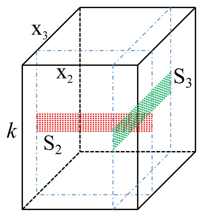
An example of the navigator data acquisition schemes for LRTES with d̂ = 3; S₂ is constructed from the red subset data and S₃ is constructed from the green subset data.

IV. Image Reconstruction

The proposed reconstruction consists of two subproblems: 1) determining the tensor subspace structure ( ${\{{\mathbf{G}}^{(i)}\}}_{i=2}^{\widehat{d}}$), and 2) determining G⁽¹⁾ and C₍₁₎.

A. Subspace estimation

The navigator data is used to determine the subspace structures. Specifically, each subset of the navigator data can be collected into a Casorati matrix S_i ∈ ℂ^N_i×M, M ≥ L_i for i ≥ 2, as illustrated in Fig. 1. This allows estimation of Ĝ⁽ⁱ⁾ ∈ ℂ^N_i×L_i from the L_i dominant left singular vectors of S_i for all i ≥ 2. We then take the subspace spanned by the columns of Ĝ⁽ⁱ⁾ as the subspace of the ith dimension in ℘.

An underlying question of the above procedure is whether the subspace spanned by the columns of Ĝ⁽ⁱ⁾ is the same as the subspace of the ith dimension in ℘. Theorem 5 in Appendix A addresses this question. Simply put, the proposed procedure requires that the signal variations along the ith dimension of the image function can be represented by the basis extracted from the navigators. Any signals that can not be represented by these bases must have signal components not visible in the set of limited k-space locations over which the navigators are measured (i.e., having a null space for these locations). We argue that such signals would not be physically meaningful if the navigators are properly collected.

B. Image Reconstruction

Let Φ̂ = (Ĝ^(d̂) ⊗ Ĝ^(d̂−1) ⊗ ⋯ ⊗ Ĝ⁽²⁾)^T, where ${\{{\widehat{\mathbf{G}}}^{(i)}\}}_{i=2}^{\widehat{d}}$ are the subspace estimates from the navigator data. For notational simplicity, let also G = G⁽¹⁾ and C = C₍₁₎. The image reconstruction problem for LRTES is then formulated as

$$\begin{array}{l}\left\{\widehat{\mathbf{G}},\widehat{\mathbf{C}}\right\}=arg\underset{\mathbf{G},\mathbf{C}}{min}{\Vert \mathbf{d}-\mathrm{\Omega }({\mathbf{FP}}_{(1)})\Vert }_2^2+R(\mathbf{G},\mathbf{C})\hfill \\ \text{s.t.}{\mathbf{P}}_{(1)}=\mathbf{GC}\widehat{\mathbf{\Phi }},\hfill \end{array},$$ (10)

where R(·) is an optional regularization functional and P̂₍₁₎ = ĜĈΦ̂ the final reconstructed image. Note that d may or may not include the navigator data according to different applications.

1) Choices of R(·)

The inclusion of R(·) provides an avenue to impose additional constraints on the structure of ℘. In this paper, we enforce different constraints on the spatial basis and core tensor jointly. The R(·) in (10) is reformulated as

$$R(\mathbf{G},\mathbf{C})=R_{\mathrm{s}}(\mathbf{C})+R_{\text{gs}}(\mathbf{G}),$$ (11)

where the penalty functions R_s(·) and R_gs(·) promote sparsity and transform group sparsity respectively.

The sparsity constraint function R_s(·) can be imposed upon the mode-1 matricization of the core tensor 𝒞 to address the nonuniqueness of the Tucker decomposition, alleviating ill-conditionedness. The strategy is to make as many elements zero (or very small) as possible in the core tensor to reduce the degrees of freedom, as is similarly done in sparse tensor approaches [48]. Furthermore, the core tensor should be sparse when the factor matrices of the tensor are made up of orthogonal columns. In LRTES, the factor matrices ${\{{\widehat{\mathbf{G}}}^{(i)}\}}_{i=2}^{\widehat{d}}$ are orthonormal bases, as they are derived from singular value decomposition of the navigator data. As a result, we adopt the sparsity constraint R_s(C) = μ||vec(C)||₁ in (11).

Since the coefficients ${\{\mathrm{\Psi }(g_{{\ell }_1}^{(1)}({\mathbf{x}}_1))\}}_{{\ell }_1=1}^{L_1}$ (for some sparsifying transform Ψ(·)) often share similar sparse support, we can impose a transform group sparsity constraint R_gs(·) on G. Group sparse modeling exploits this correlated sparse structure of spatial coefficient maps ${\{g_{{\ell }_1}^{(1)}({\mathbf{x}}_1)\}}_{{\ell }_1=1}^{L_1}$, utilizing the shared sparse support in the transform domain to form a stronger model than sparse modeling alone. Mathematically, transform group sparsity can be enforced by the mixed ℓ₁/ℓ₂ norm [49], i.e., R_gs(G) = λ||Ψ(G)||_2,1, where ||U||_2,1 = Σ_i ||u_i:||₂ and where u_i: denotes the ith row of U. We used R_gs(G) = λ||Ψ(G)||_2,1 as the group sparsity constraint when generating the results. Specifically, we implement LRTES with the sparsifying transform Ψ = ∇ = (∇_x,∇_y) (i.e., spatial finite difference operators) in this paper to enforce shared edge structure.

Under the above description, (10) can be expressed as

$$\left\{\widehat{\mathbf{G}},\widehat{\mathbf{C}}\right\}=arg\underset{\mathbf{G},\mathbf{C}}{min}{\Vert \mathbf{d}-\mathrm{\Omega }(\mathbf{FGC}\widehat{\mathbf{\Phi }})\Vert }_2^2+\lambda {\Vert \mathrm{\Psi }(\mathbf{G})\Vert }_{2,1}+\mu {\Vert \text{vec}(\mathbf{C})\Vert }_1$$ (12)

where λ, μ denote the regularization parameters.

2) Optimization algorithm

The constraints imposed by (12) are appealing from a modeling standpoint; however, the non-convex, and non-linear nature of this large-scale problem raises issues of computational complexity and local optimality. This subsection (and the appendices) address these issues, proposing an efficient and robust ADMM-based reconstruction algorithm which is simple to implement. The optimization equation in (12) can be converted into the following equivalent constrained optimization problem through variable splitting,

$$\begin{array}{r}\left\{\widehat{\mathbf{G}},\widehat{\mathbf{C}},\widehat{\mathbf{A}},\widehat{\mathbf{B}}\right\}=arg\underset{\mathbf{G},\mathbf{C},\mathbf{A},\mathbf{B}}{min}{\Vert \mathbf{d}-\mathrm{\Omega }(\mathbf{FGC}\widehat{\mathbf{\Phi }})\Vert }_2^2\\ +\lambda {\Vert \mathbf{A}\Vert }_{2,1}+\mu {\Vert \text{vec}(\mathbf{B})\Vert }_1\\ \text{s.t.}\mathbf{A}=\mathrm{\Psi }(\mathbf{G})\text{and}\mathbf{B}=\mathbf{C}\end{array}$$ (13)

The augmented Lagrangian function for (13) can then be written as

$$\begin{array}{r}\mathcal{L}(\mathbf{G},\mathbf{C},\mathbf{A},\mathbf{B},\mathbf{Y},\mathbf{Z})={\Vert \mathbf{d}-\mathrm{\Omega }(\mathbf{FGC}\widehat{\mathbf{\Phi }})\Vert }_2^2+\lambda {\Vert \mathbf{A}\Vert }_{2,1}\\ +\mu {\Vert \text{vec}(\mathbf{B})\Vert }_1+\langle \mathbf{Y},\mathbf{A}-\mathrm{\Psi }(\mathbf{G})\rangle +\langle \mathbf{Z},\mathbf{B}-\mathbf{C}\rangle \\ +\frac{\alpha }{2}{\Vert \mathbf{A}-\mathrm{\Psi }(\mathbf{G})\Vert }_F^2+\frac{\beta }{2}{\Vert \mathbf{B}-\mathbf{C}\Vert }_F^2\end{array}$$ (14)

Here, Y and Z are the two Lagrangian multipliers, and α, β > 0 are called the penalty parameters. Eq. (14) can be minimized by the following alternating direction method:

$${\mathbf{A}}_{k+1}=arg\underset{\mathbf{A}}{min}\mathcal{L}({\mathbf{G}}_k,{\mathbf{C}}_k,\mathbf{A},{\mathbf{B}}_k,{\mathbf{Y}}_k,{\mathbf{Z}}_k),$$ (15)

$${\mathbf{B}}_{k+1}=arg\underset{\mathbf{B}}{min}\mathcal{L}({\mathbf{G}}_k,{\mathbf{C}}_k,{\mathbf{A}}_{k+1},\mathbf{B},{\mathbf{Y}}_k,{\mathbf{Z}}_k),$$ (16)

$${\mathbf{G}}_{k+1}=arg\underset{\mathbf{G}}{min}\mathcal{L}(\mathbf{G},{\mathbf{C}}_k,{\mathbf{A}}_{k+1},{\mathbf{B}}_{k+1},{\mathbf{Y}}_k,{\mathbf{Z}}_k),$$ (17)

$${\mathbf{C}}_{k+1}=arg\underset{\mathbf{C}}{min}\mathcal{L}({\mathbf{G}}_{k+1},\mathbf{C},{\mathbf{A}}_{k+1},{\mathbf{B}}_{k+1},{\mathbf{Y}}_k,{\mathbf{Z}}_k),$$ (18)

$${\mathbf{Y}}_{k+1}={\mathbf{Y}}_k+\alpha ({\mathbf{A}}_{k+1}-\mathrm{\Psi }({\mathbf{G}}_{k+1})),$$ (19)

$${\mathbf{Z}}_{k+1}={\mathbf{Z}}_k+\beta ({\mathbf{B}}_{k+1}-{\mathbf{C}}_{k+1}).$$ (20)

The general solutions to the subproblems (15)–(18) are described in Appendix B.

The variables must be initialized before the above subproblems can be alternately solved. In our implementation, we initialize P₍₁₎₀ from the zero-filled reconstruction. Since P₍₁₎ = GCΦ̂ and Φ̂ contains orthonormal rows, we initialize G₀ and C₀ such that G₀C₀ = P₍₁₎₀Φ̂^H. Specifically, we initialize G₀ from the L₁ dominant left singular vectors of P₍₁₎₀Φ̂^H and then initialize ${\mathbf{C}}_0={\mathbf{G}}_0^H{\mathbf{P}}_{{(1)}_0}{\widehat{\mathbf{\Phi }}}^H$. A₀, B₀, Y₀, and Z₀ can be initialized as zero matrices.

3) Analysis of convergence

The convergence of this reconstruction algorithm applied to non-convex problems is still an open problem [50], [51]. Although empirical evidence suggests that the reconstruction algorithm has very strong convergence behavior, the satisfying proof is still under study. Here, we can give a weak convergence result that guarantees that the iteration sequence of the reconstruction algorithm converges to a first-order Karush-Kuhn-Tucker (KKT) point of (13) with mild conditions. The KKT point in this case can be either a local (or global) minimum or a saddle point. First, it is straightforward to derive the KKT conditions for (14):

$$\begin{array}{c}2{\mathrm{\Gamma }}^{\ast }(\mathbf{d}-\mathrm{\Gamma }(\mathbf{G}))+{\mathrm{\Psi }}^{\ast }(\mathbf{Y})=0;2{\mathrm{\Lambda }}^{\ast }(\mathbf{d}-\mathrm{\Lambda }(\mathbf{C}))+\mathbf{Z}=0;\\ \lambda \frac{\partial }{\partial \mathbf{A}}{\Vert \mathbf{A}\Vert }_{2,1}+\mathbf{Y}=0;\mu \frac{\partial }{\partial \mathbf{B}}{\Vert \text{vec}(\mathbf{B})\Vert }_1+\mathbf{Z}=0;\\ \mathbf{A}-\mathrm{\Psi }(\mathbf{G})=0;\mathbf{B}-\mathbf{C}=0,\end{array}$$ (21)

where Γ(G) = Ω(FGCΦ̂) and Λ(C) = Ω(FGCΦ̂).

Second, we have the following Lemma:

Lemma 1

Let W ≜ (G,C,A,B,Y,Z) and ${\{{\mathbf{W}}_k\}}_{k=1}^{\infty }$ be the sequence generated by the proposed algorithm. Assume that ${\{{\mathbf{W}}_k\}}_{k=1}^{\infty }$ is bounded and $\underset{k\to \infty }{lim}({\mathbf{W}}_{k+1}-{\mathbf{W}}_k)=0$. Then any accumulation point of ${\{{\mathbf{W}}_k\}}_{k=1}^{\infty }$ satisfies the KKT conditions. In particular, whenever ${\{{\mathbf{W}}_k\}}_{k=1}^{\infty }$ converges, it converges to a KKT point of (14).

The proof of Lemma 1 is described in Appendix C.

V. Application Examples

In this section, we applied LRTES to three high-dimensional imaging applications: multi-shell diffusion imaging, multiparameter mapping, and multidimensional spectroscopic imaging. Simulations were conducted by retrospectively undersampling either actual experimental data or numerical phantoms generated from real data. The performance of LRTES was compared with the joint sparsity-based method (denoted as Joint Sparse hereafter) in [12] and with the low-rank tensor completion in [52] (denotes as LRTC hereafter). LRTC is a tensor completion method based on minimizing the tensor trace norm (the average of the nuclear norms of all matrices unfolded along each mode). In contrast to the proposed explicit low-rank tensor model, LRTC enforces low-rankness implicitly.

A. Multi-shell diffusion imaging

Diffusion imaging has been demonstrated to be a useful tool for noninvasive quantification of tissue microstructures. In order to achieve accurate diffusion parameter estimation (especially for higher order diffusion signal models), many diffusion encoding directions with multiple b-values (also referred to as multi-shell acquisitions) are usually acquired [4], [53]. This can significantly prolong the imaging time, thus motivating accelerated acquisition.

We simulated a multi-shell diffusion imaging experiment using an adult mouse diffusion tensor atlas from the BIRN (Biomedical Informatics Research Network) Data Repository to evaluate the potential of LRTES for accelerating diffusion imaging. Specifically, the diffusion-weighted (DW) images were generated using the signal model

$$\rho (\mathbf{x},b,\mathbf{u})={\rho }_0(\mathbf{x})exp\left(-b{\mathbf{u}}^T\mathbf{D}(\mathbf{x})\mathbf{u}\right),$$ (22)

where ρ(x) is the intensity without diffusion weighting, and ${\{b_i\}}_{i=1}^{12}=\{1000,2000,3000,4000,5000,6000,7000,8000,9000,10000,11000,\text{and}12000\mathrm{s}/{\text{mm}}^2\}$ are 12 different b-values (corresponding to x₂). The ${\{{\mathbf{u}}_j\}}_{j=1}^{64}$ denote 64 different diffusion encoding directions (corresponding to the x₃), and D(x) is the diffusion tensor. We generated (1+768) images with 256 × 256 voxels, where the “1” image specifies the image without diffusion weighting (i.e., b = 0). The noise standard deviation was selected such that SNR = 9 for b = 1000 s/mm² at u₁. The SNR is defined as the ratio of mean signal to the standard deviation of noise.

Three different methods were applied to reconstruct DW images from noisy sparse samples: Joint Sparse reconstruction (group sparse modeling), LRTC (enforcing implicit low-rank tensor constraint through the nuclear norm), and LRTES. All three methods used the same variable density Cartesian sampling pattern with densely sampled 4 × 256 central k-space and a total acceleration factor (AF) = 17. The densely sampled central k-space region also covers all b-values and diffusion directions to generate S₂ and S₃, from which Ĝ⁽²⁾ and Ĝ⁽³⁾ were estimated, respectively.

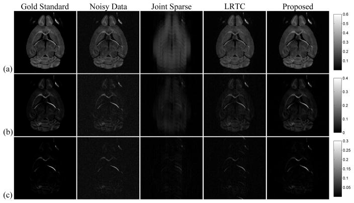
Fig. 2 shows reconstructed DW images for selected b-values at one diffusion encoding direction. As can be seen, the AF is too high for successful Joint Sparse reconstruction in all cases. The LRTES clearly outperforms LRTC with the improvement more distinct at higher b values. Note that LRTES not only accurately reconstructs the images, but also has a denoising effect, exhibiting better SNR than direct Fourier reconstruction of the fully sampled noisy data.

Fig. 2.

The representative DW images with different b-values: (a) b = 2000, (b) b = 4000, and (c) b = 7000 s/mm² for the same diffusion encoding direction, respectively; Column 1 is the gold standard, column 2 the noisy data, and column 3 to 5 the reconstructions by Joint Sparse, LRTC, and the proposed method from undersampled noisy data at AF = 17.

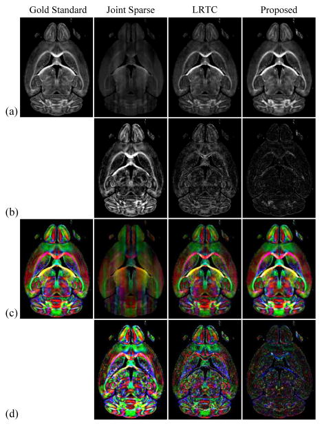
Fig. 3 compares the estimated fractional anisotropy (FA) maps and color-coded FA maps from Joint Sparse reconstruction, LRTC, and LRTES. The fully sampled image without diffusion weighting, ρ(x), and the 64 reconstructed images with different diffusion encoding directions, all with b = 1000 s/mm², were used to calculate FA using the standard least-squares approach in [54]. As Fig. 3 shows, LRTES results in the lowest error for both the FA and color-coded FA maps.

Fig. 3.

Estimated diffusion parameters from Joint Sparse, LRTC, and the proposed reconstructions at AF = 17: (a) FA maps, (b) FA error maps scaled by a factor of 2, (c) color-coded FA maps, and (d) color-coded FA error maps scaled by a factor of 2.

B. Multiparameter mapping

MR multiparameter mapping is a powerful tool for quantitative tissue characterization with applications for cancer imaging, myocardial tissue characterization, and more. Typically, this is performed by collecting multiple images with different sequence parameters and inverting the appropriate MR contrast equation to enable the estimation of the original tissue parameters (e.g., ρ, R₁, R₂, $R_2^{\ast }$). This approach, if unaccelerated, can lead to impractically long scan times.

In order to evaluate the effectiveness of the proposed method for accelerated multiparameter mapping, we created a numerical phantom from known spin density, R₁, and $R_2^{\ast }$ maps of an ex vivo rat heart. The heart was infiltrated with macrophages labeled by micron-sized particles of iron oxide (MPIO) [55] increasing both R₁ and $R_2^{\ast }$ at the site of macrophage accumulation. Relaxation rate maps R₁(x), $R_2^{\ast }(\mathbf{x})$, and spin density map A(x) were calculated from 200 × 200 MR images of the heart collected on a Bruker Avance III 7 T scanner. Using these maps, the FLASH contrast equation

$$\rho (\mathbf{x},\alpha ,T_{\mathrm{E}})=A(\mathbf{x})sin\alpha \frac{(1-exp(-T_{\mathrm{R}}{R}_1(B)))exp\left(-T_{\mathrm{E}}{R}_2^{\ast }(\mathbf{x})\right)}{1-cos\alpha exp(-T_{\mathrm{R}}{R}_1(\mathbf{x}))}$$ (23)

with T_R = 10 ms was used to generate images for the Cartesian product of sequence parameter pairings ${\{({\alpha }_i,T_{\mathrm{E},j})\}}_{i=1,j=1}^{10,11}$, where ${\{{\alpha }_i\}}_{i=1}^{10}=\{2°,5°,10°,15°,20°,25°,30°,35°,40°,\text{and}45°\}$ are the flip angles (corresponding to x₂), and ${\{T_{\mathrm{E},j}\}}_{j=1}^{11}=\{0.025,0.050,0.075,0.1,0.25,0.50,0.75,1,2.5,5,\text{and}7.5\text{ms}\}$ are the echo times (corresponding to x₃).

The same three methods as in the previous subsection were used for reconstruction. For LRTES, two subsets of navigator data were collected by densely sampling an 8 × 200 region of k-space for: a) one flip angle (45°) and all echo times; and b) one echo time (0.025 ms) and all flip angles. The remainder of (k,α,T_E)-space was sparsely sampled using variable density Gaussian sampling in k_y and uniform density sampling in α and T_E. For LRTC, the same sampling pattern was used. For Joint Sparse, a variable density Gaussian sampling pattern with densely sampled central k-space was used for all α and T_E.

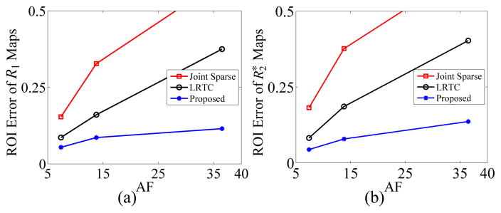
We used the variable projection (VARPRO) algorithm [56] alongside the Levenberg–Marquardt algorithm to estimate the R₁ and $R_2^{\ast }$ maps from the reconstructed images using (23). AF = 7.4, 13.8, and 36.5 were selected with SNR = 23.6 dB. The normalized root-mean-square error in the region-of-interest (ROI) was used to evaluate the performance of different reconstruction methods, where the ROI contains the MPIO-labeled macrophages.

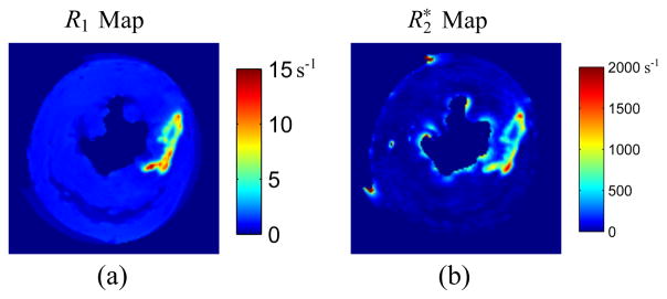
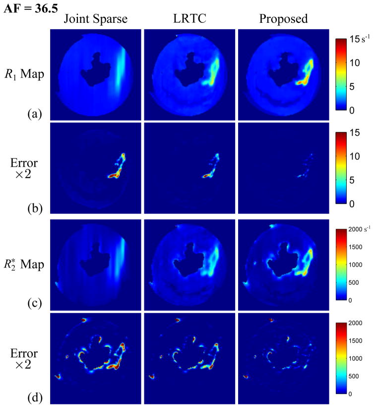
Fig. 4 shows the gold standard R₁ map and $R_2^{\ast }$ map used to generate the phantom. Fig. 5 depicts the reconstructed R₁ maps, $R_2^{\ast }$ maps, and their corresponding error maps for the rat heart at AF = 36.5 using Joint Sparse reconstruction, LRTC, and the proposed method. LRTES clearly performs the best of the three methods. Plots of the ROI error for AF = 7.4, 13.8, and 36.5 is presented in Fig. 6. LRTES shows significantly improved accuracy compared to the other two methods for both R₁ and $R_2^{\ast }$ and for all acceleration factors. The results show that LRTES yields satisfying visual and quantitative results, even at extremely high acceleration factors.

Fig. 4.

The gold standard (a) R₁ map and (b) $R_2^{\ast }$ map for the rat heart.

Fig. 5.

Reconstructed R₁ maps, $R_2^{\ast }$ maps, and their corresponding error maps for the rat heart from Joint Sparse, LRTC, and the proposed method at AF = 36.5 and SNR = 23.6 dB.

Fig. 6.

The ROI error with respect to AF: (a) ROI error of R₁ maps versus AF, and (b) $R_2^{\ast }$ maps versus AF.

We also used the gold standard multiparameter mapping dataset to demonstrate the advantage of tensor-based image representations over PS/low-rank matrix-based representation by “stacking” the data along one or more of the dimensions (detailed descriptions can be found in the supplementary materials). In short, we compared the truncated higher-order singular value decomposition (HOSVD) [57] of the entire set of multiparameter images to the truncated SVDs of each ρ(x,α_i,T_E) (i.e., each $R_2^{\ast }$-decay image sequence for a given flip angle). As seen in Fig. 3 of the supplementary materials, the two representations yield similar levels of truncation error when the tensor representation has significantly fewer degrees-of-freedom, implying low-rank tensor model’s better representation power and the potential capability in achieving higher acceleration factors.

C. Multidimensional spectroscopic imaging

Proton MR spectroscopic imaging (¹H-MRSI) allows mapping metabolite concentrations of the human brain and has wide applications in both basic scientific and clinical research. A major issue with the conventional one-dimensional ¹H-MRSI is that nearly all of the observable metabolite resonance peaks are located in a small bandwidth and overlap with each other, resulting in difficult quantification problems. This limitation can be addressed through multidimensional ¹H-MRSI, which increases the number of spectral dimensions and thus leads to larger dispersions in the spectra of metabolites [58]. A multidimensional MRSI experiment is conceptually a series of one-dimensional MRSI experiments with different imaging parameters and generally requires much longer acquisition time than the conventional MRSI experiment, limiting its application.

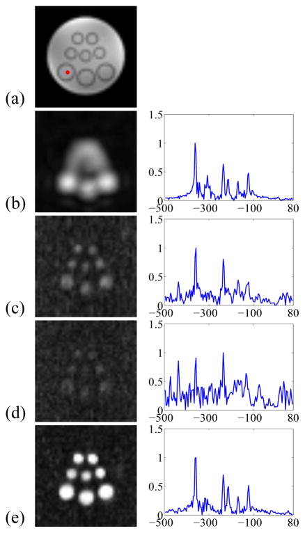
In order to evaluate the effectiveness of LRTES for accelerated multidimensional MRSI, we performed 2D J-resolved ¹H-MRSI experiments and used LRTES to reconstruct 2D J-resolved MRSI data from retrospectively undersampled data. Mathematically, the measured 2D J-resolved MRSI data can be expressed as

$$s(k_x,k_y,t_1,t_2)=\int \rho (x,y,t_1,t_2)e^{-i2\pi (k_{x}x+k_{y}y)}\mathit{dxdy}+\eta ,$$ (24)

where ρ(x,y,t₁,t₂) is the signal of interest, s(k_x,k_y,t₁,t₂) is the measured data in (k_x, k_y, t₁, t₂)-space, and η is the measurement noise (complex white Gaussian). The goal is to reconstruct ρ(x,y,t₁,t₂) from sparsely sampled (k_x, k_y, t₁, t₂)-space data. We created a brain metabolite phantom filled with NaCl-doped water and vials of different diameters (as shown in Fig. 7(a)). The vials contained solutions of Nacetylaspartate (NAA), creatine (Cr), choline (Cho), myo-inositol (mI), glutamate (glu), glutamine (gln), and gamma-aminobutyric acid (GABA) with physiologically relevant concentrations. We acquired 2D J-resolved MRSI data from the phantom on a 3T Siemens scanner using a JPRESS-EPSI sequence. A low-resolution, high-SNR, 2D J-resolved MRSI dataset was acquired with 12 (k_y) × 12 (k_x) × 20 (t₁) × 512 (t₂) encodings and 6 signal averages in a 29-minute scan. Another high-resolution, low-SNR, 2D J-resolved MRSI dataset was acquired with 64 × 64 × 20 × 128 (undersampling by a factor of 4 along t₂) encodings in a 26-minute scan. One 12 × 12 × 20 × 512 low-resolution MRSI dataset was selected as the navigator data for LRTES. The sparsely sampled dataset was sampled using variable density Gaussian sampling in k_y and uniform density sampling in t₁ with AF = 3.71 for k_y and t₁ from the high-resolution data. Joint Sparse and LRTC utilized the same sparsely sampled strategy but with AF = 2.19 to ensure the same acquisition time for these three methods.

Fig. 7.

Experimental results from the phantom shown in (a): (b): zero-padded low-resolution reconstruction, (c): Joint Sparse reconstruction, (d): LRTC reconstruction, and (e): the proposed method reconstruction. The left column shows the NAA map and the right column shows the representative spectrum (t₁ = 20ms) of the selected dot colored red in (a).

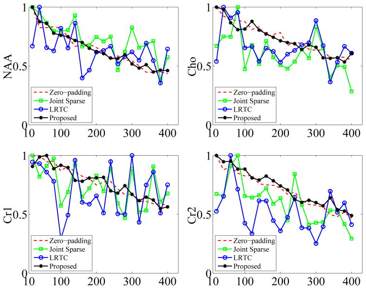
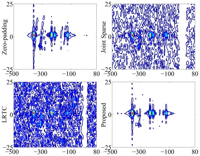
Fig. 7 shows the phantom and reconstruction results including the NAA map and representative spectrum of zero-padded low-resolution data and of three sparse sampling methods (i.e., Joint Sparse, LRTC, and the proposed method). As can be seen, the low-resolution reconstruction has high spectral resolution but suffers from serious artifacts. Among the three sparse sampling methods, LRTES achieves both very good SNR and spectral resolution. Fig. 8 presents the peak integral as a function of T_E for NAA, Cho, Cr1, and Cr2. It is clear that LRTES performs a best fitting with the zero-padded low-resolution data for each compound. Fig. 9 shows the representative 2D spectrum of the selected dot. As can be seen, LRTES yields a satisfying fit with the zero-padded low-resolution data, while Joint Sparse and LRTC have too many artifacts to recognize useful information.

Fig. 8.

Peak integral as a function of t₁ for NAA, Cho, Cr1, and Cr2.

Fig. 9.

The representative 2D spectrum of zero-padded low-resolution data, Joint Sparse, LRTC, and the proposed method for the selected dot in Fig. 7.

VI. Discussion and Conclusion

The proposed LRTES uses explicit model orders (i.e., L₁, L₂, ⋯ , L_d̂) for high-dimensional imaging. Thus, the choice of model orders ${\{L_i\}}_{i=2}^{\widehat{d}}$ that control the trade-offs between model bias and ill-conditionedness of (18) is of importance. High model orders reduce model bias at the expense of increased degrees-of-freedom and potential noise amplification while likely also requiring increased amounts of navigator data. In this work, we select ${\{L_i\}}_{i=2}^{\widehat{d}}$ by examining the singular value curves of ${\{{\mathbf{S}}_i\}}_{i=2}^{\widehat{d}}$. This has produced high-quality reconstructions in our studies, although more sophisticated schemes can be developed. Note that unlike low-rank matrix based methods, the model order L₁ for LRTES needs to be chosen separately. Our current solution to this problem is to select L₁ after initializing C₀ as described in Section IV-B2: we first initialize C₀ with a large L₁ (not to exceed L₂L₃ ⋯ L_d̂), and calculate the energy for each row of C₀. We then reset L₁ according to the falloff energy and reinitialize C₀. This algorithmic modification helps reduce model bias without unnecessarily incrementing the model order.

Another important issue of the proposed method is the choice of the regularization parameters λ and μ. With the presence of a ground truth, the regularization parameters were manually optimized to minimize the Frobenius norm of the difference between the reconstruction and the ground truth. We also observed that the performance of the proposed reconstruction is relatively stable for a range of λ and μ. Therefore, in the absence of a ground truth, we chose λ and μ by visual inspection of the reconstructed images.

It is noteworthy that when the model orders (L₂, L₃, ⋯ , L_d̂) are selected as large as (N₂, N₃, ⋯ , N_d̂), LRTES reduces to the method enforcing the low-rank constraints explicitly in a matrix form (e.g., [59]). More specifically, for all i ≥ 2, each estimated Ĝ⁽ⁱ⁾ is an orthogonal matrix due to L_i = N_i. As a result, Φ̂ = (Ĝ^(d̂) ⊗ Ĝ^(d̂−1) ⊗ ⋯ ⊗ Ĝ⁽²⁾)^T is also an orthogonal matrix, and the solution to

$$\{\widehat{\mathbf{G}},\widehat{\mathbf{C}}\}=arg\underset{\mathbf{G},\mathbf{C}}{min}{\Vert \mathbf{d}-\mathrm{\Omega }(\mathbf{FGC}\widehat{\mathbf{\Phi }})\Vert }_2^2$$ (25)

is equal to

$$\{\widehat{\mathbf{G}},\widehat{\stackrel{\sim }{\mathbf{C}}}\}=arg\underset{\mathbf{G},\stackrel{\sim }{\mathbf{C}}}{min}{\Vert \mathbf{d}-\mathrm{\Omega }(\mathbf{FG}\stackrel{\sim }{\mathbf{C}})\Vert }_2^2,$$ (26)

where G and C̃ are rank-L₁ matrices. This is equivalent to the matrix form of the original PS model as described in [20]. Compared to this low-rank matrix-based approach (with corresponding hybrid sampling strategy), exploiting the tensor structure in higher-dimensional imaging provides much more flexibility in designing accelerated data acquisition and reconstruction algorithms. Meanwhile, we expect the performance differences between these two approaches (i.e., matrix form vs. tensor form) to be application-dependent.

Regarding sampling requirements for the navigator data: as described in Section IV-A, we arrange the ith subset of navigator data into a Casorati matrix S_i ∈ ℂ^N_i×M, where M is the number of noisy observations of linear combinations of ${\{g_{{\ell }_i}^{(i)}({\mathbf{x}}_i)\}}_{{\ell }_i=1}^{L_i}$. Therefore, M theoretically only needs to be larger than L_i for i ≥ 2. In our experience, M should usually be selected greater than 2L_i to ensure a good performance. See also Theorem 5 in Appendix A for more navigator sampling considerations.

It is also worth noting the flexible imaging data sampling requirements of the proposed method. The inclusion of sparsity constraints reduces the dependence of reconstruction performance on the number of frames of imaging data, consistent with previous findings for explicit low-rank matrix imaging (e.g., [24]). Furthermore, although this paper only demonstrates variable density Gaussian sampling in k-space and uniform sampling in other dimensions, the proposed method supports a wide range of flexible sampling patterns (e.g., nonuniform sampling along the diffusion encoding dimension or the parameter dimensions), especially with the subspace pre-determined. Thus, design of an optimal sampling scheme for the proposed method in specific application contexts remains an interesting problem for future research.

The use of regularization-based formulations to enforce low-dimensional subspace constraints has been proposed in recent work (in the context of low-rank matrices) [60]. A similar tensor-subspace formulation may be another alternative way to take advantage of tensor structure, potentially reducing truncation and subspace estimation errors. This extension would require careful investigation, especially the handling of the core-tensor structure and the multiple regularization terms. Meanwhile, it is worth noting again that the proposed method has the unique advantages of (1) significant reduced degrees-of-freedom due to the explicit subspace modeling and (2) computation and memory efficiency due to the compressed representation. Furthermore, the effects of different trade-offs in bias and variance for different approaches to exploit the tensor structure need to be investigated for particular applications, which is beyond the scope of this paper. Comparison of low-rank tensor imaging to other alternative high-dimensional imaging methods should also be investigated on an application-by-application basis (e.g., comparison to other multiparameter mapping methods [61], [62]).

In conclusion, we proposed a new method for accelerated high-dimensional imaging. The method uses a novel low-rank tensor-based model to devise a special sparse sampling strategy that includes the acquisition of navigator data for defining an explicit tensor subspace structure and the acquisition of sparse data for determining the spatial coefficients and a core tensor. A sparsity constraint on the core tensor and a group transform sparsity constraint on the spatial coefficients are also incorporated in the proposed image reconstruction formulation. Results from application examples including multi-shell diffusion imaging, multiparameter mapping, and multidimensional spectroscopic imaging have demonstrated the effectiveness of the proposed method.

Appendix A Theoretical analysis for subspace estimation

In this appendix, we further analyze the subspace estimation problem. We denote S_i = P̃_(i)⊓_i, where ⊓_i is the column selection matrix for the mode-i matricization of ℘̃ (℘̃ is the tensor representation of FP₍₁₎). Assume the rank of P̃_(i) is L_i, then it can be expressed as P̃_(i) = U_iV_i, where U_i ∈ ℂ^N_i×L_i and V_i ∈ ℂ^{L_i×(N₁⋯N_(i−1)N_(i+1)⋯N_d̂)}. The rows in V_i denoted as ${\{{\mathbf{v}}_{i,\ell }\}}_{\ell }^{L_i}$ include the k-space and other variable groups except x_i. Then we have the following Theorem:

Theorem 5

For an arbitrary vector Θ = [θ₁,θ₂, ⋯ ,θ_Li] with ||Θ|| ≠ 0, if ${\displaystyle \sum _{\ell =1}^{L_i}}{\theta }_{\ell }{\mathbf{v}}_{i,\ell }{\sqcap }_i\ne 0$, then the columns of Ĝ⁽ⁱ⁾ span the same subspace of the ith physical dimension as in ℘.

Proof

Since $\mathrm{\Theta }{\mathbf{V}}_i{\sqcap }_i={\displaystyle \sum _{\ell =1}^{L_i}}{\theta }_{\ell }{\mathbf{v}}_{i,\ell }{\sqcap }_i\ne 0$ and ||Θ|| ≠ 0, the rows in V_i⊓_i are linearly independent, i.e., rank(V_i⊓_i) = L_i. As a result, rank(S_i) = rank(U_iV_i⊓_i) = rank(V_i⊓_i) = L_i. Further, we have rank(S_i) = rank(P̃_(i)).

Since Ĝ⁽ⁱ⁾ consists of the L_i dominant left singular vectors of S_i, the columns of it must span the same column subspace as in P̃_(i). This completes the proof.

Appendix B Solutions for the subproblems of (14)

The general solutions to the subproblems in (15)–(18) are established here. For the subproblems in (15) and (16), the well-known shrinkage (or soft-thresholding) formula can be applied. Then we have the elementwise solution for (15):

$$a_{ij}^{(k+1)}=\{\begin{array}{ll}\frac{{\Vert t_{i:}^{(k)}\Vert }_2-\frac{\lambda }{\alpha }}{{\Vert t_{i:}^{(k)}\Vert }_2}{t}_{ij}^{(k)},\hfill & {\Vert t_{i:}^{(k)}\Vert }_2>\frac{\lambda }{\alpha }\hfill \\ 0,\hfill & {\Vert t_{i:}^{(k)}\Vert }_2\le \frac{\lambda }{\alpha }\hfill \end{array},$$ (B.1)

where $t_{ij}^{(k)}$ is the (i, j)th entry of T_k, and ${\mathbf{T}}_k=\mathrm{\Psi }({\mathbf{G}}_k)-\frac{{\mathbf{Y}}_k}{\alpha }$.

Similarly, the elementwise solution for (16) is shown as

$$b_{ij}^{(k+1)}=\{\begin{array}{ll}\frac{c_{ij}^{(k)}-\frac{z_{ij}^{(k)}}{\beta }}{\left|c_{ij}^{(k)}-\frac{z_{ij}^{(k)}}{\beta }\right|}\left(\left|c_{ij}^{(k)}-\frac{z_{ij}^{(k)}}{\beta }\right|-\frac{\mu }{\beta }\right),\hfill & \left|c_{ij}^{(k)}-\frac{z_{ij}^{(k)}}{\beta }\right|\ge \frac{\mu }{\beta }\hfill \\ 0,\hfill & \left|c_{ij}^{(k)}-\frac{z_{ij}^{(k)}}{\beta }\right|<\frac{\mu }{\beta }\hfill \end{array}.$$ (B.2)

The solution to (17) and (18) (linear least-squares problems) can be obtained via the conjugate gradient algorithm:

$${\mathbf{G}}_{k+1}={\left({{\mathrm{\Gamma }}_k}^{\ast }{\mathrm{\Gamma }}_k+\frac{\alpha }{2}{\mathrm{\Psi }}^{\ast }\mathrm{\Psi }\right)}^{-1}\left({{\mathrm{\Gamma }}_k}^{\ast }(\mathbf{d})+\frac{\alpha }{2}{\mathrm{\Psi }}^{\ast }({\mathbf{A}}_{k+1}+\frac{{\mathbf{Y}}_k}{\alpha })\right).$$ (B.3)

$${\mathbf{C}}_{k+1}={\left({{\mathrm{\Lambda }}_k}^{\ast }{\mathrm{\Lambda }}_k+\frac{\beta }{2}\mathbf{I}\right)}^{-1}\left({{\mathrm{\Lambda }}_k}^{\ast }(\mathbf{d})+\frac{\beta }{2}({\mathbf{B}}_{k+1}+\frac{{\mathbf{Z}}_k}{\beta })\right),$$ (B.4)

where Γ_k(G) = Ω(FGC_kΦ̂) and Λ_k(C) = Ω(FG_k+1CΦ̂) are the linear operators and I the identity operator.

Appendix C Proof of Lemma 1

In this appendix, we give the proof of Lemma 1.

Proof

It follows from (B.1) and the identity $t_{ij}^{(k)}=\mathrm{\Psi }{({\mathbf{G}}_k)}_{ij}-y_{ij}^{(k)}/\alpha$ that

$$a_{ij}^{(k+1)}-a_{ij}^{(k)}=\{\begin{array}{ll}{t}_{ij}^{(k)}-a_{ij}^{(k)}-\frac{\lambda }{\alpha }\frac{t_{ij}^{(k)}}{{\Vert t_{i:}^{(k)}\Vert }_2},\hfill & {\Vert t_{i:}^{(k)}\Vert }_2>\frac{\lambda }{\alpha }\hfill \\ -a_{ij}^{(k)},\hfill & {\Vert t_{i:}^{(k)}\Vert }_2\le \frac{\lambda }{\alpha }\hfill \end{array}$$

Since $\frac{t_{ij}^{(k)}}{{\Vert t_{i:}^{(k)}\Vert }_2}=\frac{a_{ij}^{(k+1)}}{{\Vert a_{i:}^{(k+1)}\Vert }_2}$ for ${\Vert t_{i:}^{(k)}\Vert }_2>\frac{\lambda }{\alpha }$, for $a_{ij}^{(k+1)}\ne 0$, we have

$$a_{ij}^{(k+1)}-a_{ij}^{(k)}=\mathrm{\Psi }{({\mathbf{G}}_k)}_{ij}-a_{ij}^{(k)}-\frac{1}{\alpha }\left(y_{ij}^{(k)}+\lambda \frac{a_{ij}^{(k+1)}}{{\Vert a_{i:}^{(k+1)}\Vert }_2}\right).$$ (C.1)

Similarly, according to (B.2), it follows that

$$b_{ij}^{(k+1)}-b_{ij}^{(k)}=\{\begin{array}{ll}{c}_{ij}^{(k)}-b_{ij}^{(k)}-\frac{z_{ij}^{(k)}}{\beta }-\frac{\mu }{\beta },\hfill & b_{ij}^{(k+1)}>0\hfill \\ -b_{ij}^{(k)},\hfill & b_{ij}^{(k+1)}=0\hfill \\ c_{ij}^{(k)}-b_{ij}^{(k)}-\frac{z_{ij}^{(k)}}{\beta }+\frac{\mu }{\beta },\hfill & b_{ij}^{(k+1)}<0\hfill \end{array}$$

For $b_{ij}^{(k+1)}\ne 0$, we have

$$b_{ij}^{(k+1)}-b_{ij}^{(k)}=c_{ij}^{(k)}-b_{ij}^{(k)}-\frac{1}{\beta }\left(z_{ij}^{(k)}+\mu ·sgn(b_{ij}^{(k+1)})\right).$$ (C.2)

Also, with (B.3), (B.4), and the identities Γ_k(G) = Ω(FGC_kΦ̂) and Λ_k(C) = Ω(FG_k+1CΦ̂), we have

$$\left({{\mathrm{\Gamma }}_k}^{\ast }{\mathrm{\Gamma }}_k+\frac{\alpha }{2}{\mathrm{\Psi }}^{\ast }\mathrm{\Psi }\right)({\mathbf{G}}_{k+1}-{\mathbf{G}}_k)={{\mathrm{\Gamma }}_k}^{\ast }(\mathbf{d}-{\mathrm{\Gamma }}_k({\mathbf{G}}_k))+\frac{{\mathrm{\Psi }}^{\ast }({\mathbf{Y}}_k)}{2}+\frac{\alpha }{2}({\mathrm{\Psi }}^{\ast }({\mathbf{A}}_{k+1}-\mathrm{\Psi }({\mathbf{G}}_k)))$$ (C.3)

$$\left({{\mathrm{\Lambda }}_k}^{\ast }{\mathrm{\Lambda }}_k+\frac{\beta }{2}\mathbf{I}\right)({\mathbf{C}}_{k+1}-{\mathbf{C}}_k)={{\mathrm{\Lambda }}_k}^{\ast }(\mathbf{d}-{\mathrm{\Lambda }}_k({\mathbf{C}}_k))+\frac{{\mathbf{Z}}_k}{2}+\frac{\beta }{2}({\mathbf{B}}_{k+1}-{\mathbf{C}}_k)$$ (C.4)

It also follows from (19) and (20) that

$${\mathbf{Y}}_{k+1}-{\mathbf{Y}}_k=\alpha ({\mathbf{A}}_{k+1}-\mathrm{\Psi }({\mathbf{G}}_{k+1}))$$ (C.5)

$${\mathbf{Z}}_{k+1}-{\mathbf{Z}}_k=\beta ({\mathbf{B}}_{k+1}-{\mathbf{C}}_{k+1}).$$ (C.6)

With the assumption that ${\{{\mathbf{W}}_k\}}_{k=1}^{\infty }$ is bounded and $\underset{k\to \infty }{lim}({\mathbf{W}}_{k+1}-{\mathbf{W}}_k)=0$, the left-hand sides of (C.1)–(C.6) tend to zero as k → ∞. Consequently,

$$\begin{array}{c}\lambda a_{ij}^{(k+1)}/{\Vert a_{i:}^{(k+1)}\Vert }_2+y_{ij}^{(k)}\to 0;\mu ·sgn\left(b_{ij}^{(k+1)}\right)+z_{ij}^{(k)}\to 0;\\ 2{{\mathrm{\Gamma }}_k}^{\ast }(\mathbf{d}-{\mathrm{\Gamma }}_k({\mathbf{G}}_k))+{\mathrm{\Psi }}^{\ast }({\mathbf{Y}}_k)\to 0;2{{\mathrm{\Lambda }}_k}^{\ast }(\mathbf{d}-{\mathrm{\Lambda }}_k({\mathbf{C}}_k))+{\mathbf{Z}}_k\to 0;\\ {\mathbf{A}}_{k+1}-\mathrm{\Psi }({\mathbf{G}}_{k+1})\to 0;{\mathbf{B}}_{k+1}-{\mathbf{C}}_{k+1}\to 0,\end{array}$$ (C.7)

where the last two limits in (C.7) are used to derive other limits. That is, the sequence asymptotically satisfies the KKT condition (21). This completes the proof.

References

- 1.Finn JP, Nael K, Deshpande V, Ratib O, Laub G. Cardiac MR imaging: State of the technology. Radiol. 2006;241(2):338–354. doi: 10.1148/radiol.2412041866. [DOI] [PubMed] [Google Scholar]
- 2.Ma D, Gulani V, Seiberlich N, Liu K, Sunshine JL, Duerk JL, Griswold MA. Magnetic resonance fingerprinting. Nature. 2013;495(7440):187–192. doi: 10.1038/nature11971. [DOI] [PMC free article] [PubMed] [Google Scholar]
- 3.Posse S, Otazo R, Dager SR, Alger J. MR spectroscopic imaging: principles and recent advances. J Magn Reson. 2013;37(6):1301–1325. doi: 10.1002/jmri.23945. [DOI] [PMC free article] [PubMed] [Google Scholar]
- 4.Descoteaux M, Deriche R, Le Bihan D, Mangin JF, Poupon C. Multiple q-shell diffusion propagator imaging. Med Image Anal. 2011;15(4):603–621. doi: 10.1016/j.media.2010.07.001. [DOI] [PubMed] [Google Scholar]
- 5.Feng P, Bresler Y. Spectrum-blind minimum-rate sampling and reconstruction of multiband signals. Proc. IEEE Int. Conf. Acoust. Speech Signal Process; IEEE; 1996. pp. 1688–1691. [Google Scholar]
- 6.Candès EJ, Romberg J, Tao T. Robust uncertainty principles: Exact signal reconstruction from highly incomplete frequency information. IEEE Trans Inf Theory. 2006;52(2):489–509. [Google Scholar]
- 7.Candes EJ, Tao T. Near-optimal signal recovery from random projections: Universal encoding strategies? IEEE Trans Inf Theory. 2006;52(12):5406–5425. [Google Scholar]
- 8.Donoho DL. Compressed sensing. IEEE Trans Inf Theory. 2006;52(4):1289–1306. [Google Scholar]
- 9.Lustig M, Donoho D, Pauly JM. Sparse MRI: The application of compressed sensing for rapid MR imaging. Magn Reson Med. 2007;58(6):1182–1195. doi: 10.1002/mrm.21391. [DOI] [PubMed] [Google Scholar]
- 10.Wang H, Liang D, King K, Ying L. Toeplitz random encoding for reduced acquisition using compressed sensing. Proc. ISMRM; Honolulu, Hi. 2009; p. 2669. [Google Scholar]
- 11.Haldar JP, Hernando D, Liang ZP. Compressed-sensing MRI with random encoding. IEEE Trans Med Imag. 2011;30(4):893–903. doi: 10.1109/TMI.2010.2085084. [DOI] [PMC free article] [PubMed] [Google Scholar]
- 12.Majumdar A, Ward RK. Accelerating multi-echo T2 weighted MR imaging: Analysis prior group-sparse optimization. J Magn Reson. 2011;210(1):90–97. doi: 10.1016/j.jmr.2011.02.015. [DOI] [PubMed] [Google Scholar]
- 13.Liang D, DiBella EV, Chen RR, Ying L. k-t ISD: Dynamic cardiac MR imaging using compressed sensing with iterative support detection. Mag Reson Med. 2012;68(1):41–53. doi: 10.1002/mrm.23197. [DOI] [PMC free article] [PubMed] [Google Scholar]
- 14.Chen GH, Tang J, Leng S. Prior image constrained compressed sensing (piccs): a method to accurately reconstruct dynamic CT images from highly undersampled projection data sets. Med Phys. 2008;35(2):660–663. doi: 10.1118/1.2836423. [DOI] [PMC free article] [PubMed] [Google Scholar]
- 15.Vaswani N, Lu W. Modified-CS: Modifying compressive sensing for problems with partially known support. IEEE Trans Signal Process. 2010;58(9):4595–4607. [Google Scholar]
- 16.Liang D, Liu B, Wang J, Ying L. Accelerating sense using compressed sensing. Med Reson Med. 2009;62(6):1574–1584. doi: 10.1002/mrm.22161. [DOI] [PubMed] [Google Scholar]
- 17.Adluru G, McGann C, Speier P, Kholmovski EG, Shaaban A, DiBella EV. Acquisition and reconstruction of undersampled radial data for myocardial perfusion magnetic resonance imaging. J Magn Reson Imag. 2009;29(2):466–473. doi: 10.1002/jmri.21585. [DOI] [PMC free article] [PubMed] [Google Scholar]
- 18.Kim YC, Narayanan SS, Nayak KS. Accelerated three-dimensional upper airway MRI using compressed sensing. Med Reson Med. 2009;61(6):1434–1440. doi: 10.1002/mrm.21953. [DOI] [PMC free article] [PubMed] [Google Scholar]
- 19.Otazo R, Kim D, Axel L, Sodickson DK. Combination of compressed sensing and parallel imaging for highly accelerated first-pass cardiac perfusion MRI. Med Reson Med. 2010;64(3):767–776. doi: 10.1002/mrm.22463. [DOI] [PMC free article] [PubMed] [Google Scholar]
- 20.Liang Z-P. Spatiotemporal imaging with partially separable functions. Proc. IEEE Int. Symp. Biomed. Imag; 2007; pp. 988–991. [Google Scholar]
- 21.Haldar JP, Liang Z-P. Spatiotemporal imaging with partially separable functions: A matrix recovery approach. Proc. IEEE Int. Symp. Biomed. Imag; IEEE; 2010. pp. 716–719. [Google Scholar]
- 22.Pedersen H, Kozerke S, Ringgaard S, Nehrke K, Kim WY. k-t PCA: Temporally constrained k-t BLAST reconstruction using principal component analysis. Magn Reson Med. 2009;62(3):706–716. doi: 10.1002/mrm.22052. [DOI] [PubMed] [Google Scholar]
- 23.Lingala SG, Hu Y, DiBella E, Jacob M. Accelerated dynamic MRI exploiting sparsity and low-rank structure: k-t SLR. IEEE Trans Med Imag. 2011;30(5):1042–1054. doi: 10.1109/TMI.2010.2100850. [DOI] [PMC free article] [PubMed] [Google Scholar]
- 24.Zhao B, Haldar JP, Christodoulou AG, Liang ZP. Image reconstruction from highly undersampled (k,t)-space data with joint partial separability and sparsity constraints. IEEE Trans Med Imag. 2012;31(9):1809–1820. doi: 10.1109/TMI.2012.2203921. [DOI] [PMC free article] [PubMed] [Google Scholar]
- 25.Liang ZP, Jiang H, Hess CP, Lauterbur PC. Dynamic imaging by model estimation. Int J Imag Syst Tech. 1997;8(6):551–557. [Google Scholar]
- 26.Gupta AS, Liang Z. Dynamic imaging by temporal modeling with principal component analysis. Proc. 9th Ann. Meet. Int. Soc. Magn. Reson. Med; 2001; p. 10. [Google Scholar]
- 27.Trzasko JD, Manduca A. Clear: Calibration-free parallel imaging using locally low-rank encouraging reconstruction. Proc. Int. Soc. Magn. Reson. Med; 2012; p. 517. [Google Scholar]
- 28.Zhang T, Pauly JM, Levesque IR. Accelerating parameter mapping with a locally low rank constraint. Med Reson Med. 2015;73(2):655–661. doi: 10.1002/mrm.25161. [DOI] [PMC free article] [PubMed] [Google Scholar]
- 29.Otazo R, Candès E, Sodickson DK. Low-rank plus sparse matrix decomposition for accelerated dynamic MRI with separation of background and dynamic components. Magn Reson Med. 2015;73(3):1125–1136. doi: 10.1002/mrm.25240. [DOI] [PMC free article] [PubMed] [Google Scholar]
- 30.Christodoulou AG, Zhang H, Zhao B, Hitchens TK, Ho C, Liang ZP. High-resolution cardiovascular MRI by integrating parallel imaging with low-rank and sparse modeling. IEEE Trans Biomed Eng. 2013;60(11):3083–3092. doi: 10.1109/TBME.2013.2266096. [DOI] [PMC free article] [PubMed] [Google Scholar]
- 31.Fu M, Zhao B, Carignan C, Shosted RK, Perry JL, Kuehn DP, Liang ZP, Sutton BP. High-resolution dynamic speech imaging with joint low-rank and sparsity constraints. Magn Reson Med. 2015;73(5):1820–1832. doi: 10.1002/mrm.25302. [DOI] [PMC free article] [PubMed] [Google Scholar]
- 32.Gao H, Li L, Zhang K, Zhou W, Hu X. PCLR: Phase-constrained low-rank model for compressive diffusion-weighted MRI. Med Reson Med. 2014;72(5):1330–1341. doi: 10.1002/mrm.25052. [DOI] [PMC free article] [PubMed] [Google Scholar]
- 33.Zhao B, Lu W, Hitchens TK, Lam F, Ho C, Liang ZP. Accelerated mr parameter mapping with low-rank and sparsity constraints. Med Reson Med. 2014 doi: 10.1002/mrm.25421. [DOI] [PMC free article] [PubMed] [Google Scholar]
- 34.Lam F, Liang ZP. A subspace approach to high-resolution spectroscopic imaging. Magn Reson Med. 2014;71(4):1349–1357. doi: 10.1002/mrm.25168. [DOI] [PMC free article] [PubMed] [Google Scholar]
- 35.Gao H, Yu H, Osher S, Wang G. Multi-energy CT based on a prior rank, intensity and sparsity model (PRISM) Inverse Probl. 2011;27(11):115012. doi: 10.1088/0266-5611/27/11/115012. [DOI] [PMC free article] [PubMed] [Google Scholar]
- 36.Trzasko JD, Manduca A. A unified tensor regression framework for calibrationless dynamic, multi-channel MRI reconstruction. Proc. Int. Soc. Magn. Reson. Med; 2013; p. 603. [Google Scholar]
- 37.Yu Y, Jin J, Liu F, Crozier S. Multidimensional compressed sensing MRI using tensor decomposition-based sparsifying transform. PLoS One. 2014;9(6):e98441. doi: 10.1371/journal.pone.0098441. [DOI] [PMC free article] [PubMed] [Google Scholar]
- 38.Lei J, Liu W, Liu S, Wang X. Dynamic imaging method using the low n-rank tensor for electrical capacitance tomography. Flow Meas Instrum. 2015;41:104–114. [Google Scholar]
- 39.Mardani M, Ying L, Giannakis GB. Accelerating dynamic MRI via tensor subspace learning. Proc. Int. Soc. Magn. Reson. Med; 2015; p. 3808. [Google Scholar]
- 40.Kolda TG, Bader BW. Tensor decompositions and applications. SIAM Rev. 2009;51(3):455–500. [Google Scholar]
- 41.Reed M, Simon B, Reed M, Simon B, Reed M, Simon B, Simon B. Methods of Modern Mathematical Physics. I: Functional Analysis. New York: Academic; 1972. [Google Scholar]
- 42.Kline M. Mathematical Thought from Ancient to Modern Times. Vol. 3 Oxford Univ. Press; 1990. [Google Scholar]
- 43.Carroll JD, Chang JJ. Analysis of individual differences in multidimensional scaling via an N-way generalization of ‘Eckart-Young’ decomposition. Psychometrika. 1970;35(3):283–319. [Google Scholar]
- 44.Tucker LR. Some mathematical notes on three-mode factor analysis. Psychometrika. 1966;31(3):279–311. doi: 10.1007/BF02289464. [DOI] [PubMed] [Google Scholar]
- 45.De Silva V, Lim LH. Tensor rank and the ill-posedness of the best low-rank approximation problem. SIAM J Matrix Anal Appl. 2008;30(3):1084–1127. [Google Scholar]
- 46.Christodoulou AG, Hitchens TK, Wu Y, Ho C, Liang ZP. Improved subspace estimation for low-rank model-based accelerated cardiac imaging. IEEE Trans Biomed Eng. 2014 Sep;61(9):2451–2457. doi: 10.1109/TBME.2014.2320463. [DOI] [PMC free article] [PubMed] [Google Scholar]
- 47.Brinegar C, Schmitter SS, Mistry NN, Johnson GA, Liang ZP. Improving temporal resolution of pulmonary perfusion imaging in rats using the partially separable functions model. Magn Reson Med. 2010;64(4):1162–1170. doi: 10.1002/mrm.22500. [DOI] [PMC free article] [PubMed] [Google Scholar]
- 48.Caiafa CF, Cichocki A. Multidimensional compressed sensing and their applications. Wiley Interdiscip Rev Data Min Knowl Discov. 2013;3(6):355–380. [Google Scholar]
- 49.Jenatton R, Audibert JY, Bach F. Structured variable selection with sparsity-inducing norms. J Mach Learn Res. 2011;12:2777–2824. [Google Scholar]
- 50.Shen Y, Wen Z, Zhang Y. Augmented lagrangian alternating direction method for matrix separation based on low-rank factorization. Optim Methods Softw. 2014;29(2):239–263. [Google Scholar]
- 51.Liu Q, Liang D, Song Y, Luo J, Zhu Y, Li W. Augmented lagrangian-based sparse representation method with dictionary updating for image deblurring. SIAM J Imag Sci. 2013;6(3):1689–1718. [Google Scholar]
- 52.Liu J, Musialski P, Wonka P, Ye J. Tensor completion for estimating missing values in visual data. IEEE Trans Pattern Anal Mach Intell. 2013;35(1):208–220. doi: 10.1109/TPAMI.2012.39. [DOI] [PubMed] [Google Scholar]
- 53.Aganj I, Lenglet C, Sapiro G, Yacoub E, Ugurbil K, Harel N. Reconstruction of the orientation distribution function in single-and multiple-shell q-ball imaging within constant solid angle. Magn Reson Med. 2010;64(2):554–566. doi: 10.1002/mrm.22365. [DOI] [PMC free article] [PubMed] [Google Scholar]
- 54.Koay CG, Chang LC, Carew JD, Pierpaoli C, Basser PJ. A unifying theoretical and algorithmic framework for least squares methods of estimation in diffusion tensor imaging. J Magn Reson. 2006;182(1):115–125. doi: 10.1016/j.jmr.2006.06.020. [DOI] [PubMed] [Google Scholar]
- 55.Wu YL, Ye Q, Foley LM, Hitchens TK, Sato K, Williams JB, Ho C. In situ labeling of immune cells with iron oxide particles: an approach to detect organ rejection by cellular MRI. Proc Natl Acad Sci USA. 2006;103(6):1852–1857. doi: 10.1073/pnas.0507198103. [DOI] [PMC free article] [PubMed] [Google Scholar]
- 56.Golub G, Pereyra V. Separable nonlinear least squares: The variable projection method and its applications. Inverse Probl. 2003;19(2):R1. [Google Scholar]
- 57.De Lathauwer L, De Moor B, Vandewalle J. A multilinear singular value decomposition. SIAM J Matrix Anal Appl. 2000;21(4):1253–1278. [Google Scholar]
- 58.Wilson NE, Iqbal Z, Burns BL, Keller M, Thomas MA. Accelerated five-dimensional echo planar J-resolved spectroscopic imaging: Implementation and pilot validation in human brain. Magn Reson Med. 2016;75(1):42–51. doi: 10.1002/mrm.25605. [DOI] [PubMed] [Google Scholar]
- 59.Zhao B, Haldar JP, Brinegar C, Liang Z-P. Low rank matrix recovery for real-time cardiac MRI. Proc. IEEE Int. Symp. Biomed. Imag; IEEE; 2010. pp. 996–999. [Google Scholar]
- 60.Velikina JV, Samsonov AA. Reconstruction of dynamic image series from undersampled MRI data using data-driven model consistency condition (MOCCO) Magn Reson Med. 2015;74(5):1279–1290. doi: 10.1002/mrm.25513. [DOI] [PMC free article] [PubMed] [Google Scholar]
- 61.Block KT, Uecker M, Frahm J. Model-based iterative reconstruction for radial fast spin-echo MRI. IEEE Trans Med Imag. 2009;28(11):1759–1769. doi: 10.1109/TMI.2009.2023119. [DOI] [PubMed] [Google Scholar]
- 62.Velikina JV, Alexander AL, Samsonov A. Accelerating MR parameter mapping using sparsity-promoting regularization in parametric dimension. Magn Reson Med. 2013;70(5):1263–1273. doi: 10.1002/mrm.24577. [DOI] [PMC free article] [PubMed] [Google Scholar]
Associated Data
This section collects any data citations, data availability statements, or supplementary materials included in this article.