Abstract
Brain functional network analysis has shown great potential in understanding brain functions and also in identifying biomarkers for brain diseases, such as Alzheimer's disease (AD) and its early stage, mild cognitive impairment (MCI). In these applications, accurate construction of biologically meaningful brain network is critical. Sparse learning has been widely used for brain network construction; however, its l 1‐norm penalty simply penalizes each edge of a brain network equally, without considering the original connectivity strength which is one of the most important inherent linkwise characters. Besides, based on the similarity of the linkwise connectivity, brain network shows prominent group structure (i.e., a set of edges sharing similar attributes). In this article, we propose a novel brain functional network modeling framework with a “connectivity strength‐weighted sparse group constraint.” In particular, the network modeling can be optimized by considering both raw connectivity strength and its group structure, without losing the merit of sparsity. Our proposed method is applied to MCI classification, a challenging task for early AD diagnosis. Experimental results based on the resting‐state functional MRI, from 50 MCI patients and 49 healthy controls, show that our proposed method is more effective (i.e., achieving a significantly higher classification accuracy, 84.8%) than other competing methods (e.g., sparse representation, accuracy = 65.6%). Post hoc inspection of the informative features further shows more biologically meaningful brain functional connectivities obtained by our proposed method. Hum Brain Mapp 38:2370–2383, 2017. © 2017 Wiley Periodicals, Inc.
Keywords: brain network, sparse representation, functional connectivity, mild cognitive impairment (MCI), disease classification
INTRODUCTION
Study of brain functional network based on resting‐state functional magnetic resonance imaging (rs‐fMRI) has shown great potential in understanding brain functions and also identifying biomarkers for neurological and psychiatric disorders (Fornito et al., 2015; Wernick et al., 2010). Accurate construction of brain functional network from regional rs‐fMRI time series is an essential step prior to the subsequent statistical analysis or disease classification (Eguiluz et al., 2005; Rubinov and Sporns, 2010; Van Den Heuvel and Pol, 2010). Many approaches for brain functional network modeling have been proposed in the past (Smith et al., 2011). One of the most popular ways is to represent a brain network as a graph that comprises nodes and edges (Sporns et al., 2004; Supekar et al., 2008). The definitions of nodes and edges in a graph may differ in scale, but in this article, we construct a macroscopic brain functional network by treating the brain regions, or regions of interest (ROIs) from predefined atlas (Craddock et al., 2012; Tzourio‐Mazoyer et al., 2002), as nodes and the functional connectivity (estimated using the observed regional mean blood‐oxygen‐level‐dependent [BOLD] time series) between each pair of regions as an edge (Smith et al., 2011).
With the above definitions, the most popular approaches for brain network modeling are based on inter‐regional Pearson's correlation (PC) (Hampson et al., 2002; Power et al., 2011; Wee et al., 2012) and partial correlation (Fransson and Marrelec, 2008; Salvador et al., 2005). While the former is easy to understand and can capture pairwise functional relationship based on a pair of regions, the latter can account for more complex interactions among multiple brain regions. But the estimation of partial correlation involves an inversion of a covariance matrix, which may be ill‐posed due to the singularity of the covariance matrix. To overcome this issue, a number of representative approaches with ‐norm regularization have been introduced by adding a sparsity term since the brain network is believed to be sparse, i.e., some insignificant or spurious connections caused by the low frequency (<0.1 Hz) fluctuation of BOLD signals (Fransson, 2005) and physiological noise are forced to be zero, thus making the constructed sparse connectivity relatively easier to be interpreted. To a certain extent, the constructed sparse brain network is neurologically justified by the fact that brain regions have only “first‐order/direct” interactions with a few regions, instead of connecting with all brain regions. Two major types of representative approaches, i.e., l 1‐norm regularized maximum likelihood estimation (Huang et al., 2009; Rosa et al., 2015; Yuan and Lin, 2006), a.k.a. graphical LASSO (Friedman et al., 2008), and l 1‐norm regularized linear regression or sparse representation (SR) (Meinshausen and Bühlmann, 2006; Peng et al., 2009), have been widely applied to construct brain network for brain disease studies, such as Alzheimer's disease (AD), mild cognitive impairment (MCI) (Huang et al., 2010), and autism spectrum disorder (Lee et al., 2011). More recent representative approaches also take group structure into consideration by adding a group sparsity constraint because of the modular structure of the human brain (Rubinov and Sporns, 2010). To further introduce sparsity within each group, sparse group representation (SGR) has been developed by combining ‐norm and ‐norm constraints, which finally achieves both inter‐ and intra‐group sparsity (Jiang et al., 2015).
A common issue of all the aforementioned sparsity‐based network construction methods is that the sparse constraint term penalizes each edge equally. In other words, when learning SR for a target ROI, the BOLD signals from all other ROIs are treated equally. Such process ignores the inherent similarity between BOLD signals of the target ROI and the other ROIs during network reconstruction. Consequently, this will usually result in a sparse but difficult‐to‐understand “brain network”. We assume in this article that a target ROI's signal is prone to be represented by signals from the ROIs whose BOLD activities are highly synchronized with the target ROI. Based on this assumption, the constructed sparse brain functional network may be more reasonable. On the other hand, not all the weak links to the target ROI have to be removed. Instead, with a delicately designed learning‐based framework, the connectivity network can be learned by minimizing an objective function consisting of both a data‐fitting term and a “weighted” sparse regularization term. In this way, some ROIs with signals weakly correlated to the target ROI can still be kept, as long as they can largely reduce the data‐fitting error. In this article, we combine the merits of both pairwise correlations and the SR to better model the brain functional network. Specifically, we make better use of the pairwise correlation from PC to drive sparse model, instead of simply discarding this important information. In light of this, we introduce a “functional connectivity strength‐related” penalty in SR, namely, weighted sparse representation (WSR).
Figure 1 shows the simple example of brain networks constructed by PC, SR, and our proposed WSR from real fMRI data. In this proof‐of‐concept case, the PC‐based network is denser compared with the two SR‐based networks (by SR and our proposed WSR method, respectively). Due to equal penalization, the network constructed by SR looks as noisy as a random network, probably due to the fact that it often misses many important connections that should have close relationships. In contrast, by considering pairwise functional connectivity strength (derived from PC) in sparse coding, the links with strong connectivity strength are less penalized. By retaining both sparsity and connectivity prior, the network constructed by the WSR is thus more biologically meaningful (i.e., having a clearly structured connectivity matrix or modular architecture). This is because that the relationship between two regions is measured by considering both pairwise correlation and the contribution of other regions. Moreover, to further make the penalty consistent within each subset of links with similar pairwise connectivity strength, we additionally propose a group structure‐based constraint in the model. In this way, similar links will share similar penalties during network construction. Thus, we can jointly model the whole‐brain network, instead of independently modeling each ROI; in this way, each ROI's construction will gain benefit from other ROIs’ constructions. This joint estimation strategy can result in more biologically meaningful brain functional network. We call our method “connectivity strength‐weighted sparse group representation (WSGR),” which integrates (1) sparsity, (2) functional connectivity strength, and (3) group structure in a unified framework.
Figure 1.
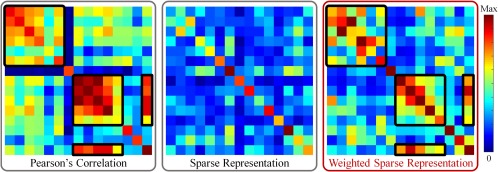
Illustration of our motivation. Note that these networks are obtained from real rs‐fMRI data (where all values are absolute). The black boxes in the matrices are used to show the corresponding effect of the connectivity strength‐based weights in the constructed brain network. [Color figure can be viewed at http://wileyonlinelibrary.com]
We hypothesize that, based on our method, brain network construction will be more reasonable and better reflect the true functional organization architecture of the human brain. To validate this, we conduct experiments on real fMRI data, construct different brain functional networks based on our method and other competing methods (PC, SR, and SGR), and use these networks to conduct individualized diagnosis of brain disorder (i.e., distinguishing MCI subjects from normal controls). The results show that our method, even with simple feature selection and linear support vector machine (SVM), achieves superior classification performance compared with other methods. The selected features (i.e., network connections) can be utilized as potential biomarkers to guide early intervention of AD in the future.
The remainder of this article is organized as follows. In Section 2, we detail the proposed brain network construction model. Then, we apply the constructed brain network for MCI classification in Section 3. The experiments and results will be given in Section 4, followed by discussions and summary in Sections 5 and 6, respectively.
WSGR‐BASED BRAIN NETWORK CONSTRUCTION
In this work, we propose a WSGR for brain functional network construction, which considers traditional correlation as connectivity strength to guide sparse modeling for brain network construction. Overview of the proposed construction framework is shown in Figure 2.
Figure 2.
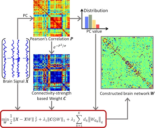
Framework of the proposed brain functional network construction. Given brain functional signals , we can compute a Pearson's correlation (PC) matrix , which will be used to define both the connectivity strength weight for the ‐norm and the group partition for the ‐norm in the proposed model. The brain network will be constructed with optimization. [Color figure can be viewed at http://wileyonlinelibrary.com]
In a classical brain functional network construction problem, the brain can be parcellated into N ROIs according to a certain brain atlas. The regional mean time series of the ROI can be denoted by a column vector , where M is the number of time points in the entire time series, and thus denotes the data matrix of a subject. By modeling brain functional network as a graph, a key step is to estimate the connectivity matrix , given the N nodes (i.e., ), each representing an ROI's signal.
The traditional sparse brain network modeling of the ROI can be formulated as a standard ‐norm regularized optimization problem, and the whole‐brain network construction can be defined as
| (1) |
where is the estimated functional connectivity between and after excluding the confounding effects of other regions.
Connectivity Strength‐Based Weighting and Weighted Sparse Representation (WSR)
The ‐norm regularization involved in Eq. (1) (the second term) penalizes each representation coefficient ( ) with the same weight of one. In other words, it treats each ROI equally when reconstructing signals ( ) for a target ROI. Thus, the inherent pairwise correlation with respect to , i.e., “functional connectivity strength,” is completely discarded during the optimization. As a result, this type of sparse modeling methods may tend to select only the ROIs with weak connectivities to the target ROI, as long as this can minimize the objective function in Eq. (1). Moreover, the representation of one ROI is independent of the representations of other ROIs. This “independent representation” can lead to less biologically meaningful brain network. The estimated representation coefficients of the functionally similar ROIs could vary largely in an unconstrained way. Considering these issues, we argue that the prior functional connectivity strength should be incorporated into the brain functional network construction.
Specifically, we can introduce a connectivity strength‐weighted sparse penalty in Eq. (1) to take the strength of functional connectivity into account. We suppose that if the BOLD signals of two ROIs have a high correlation, indicating a strong link between each other, then this strong functional link should be less penalized to make it more possible to be chosen to represent the target ROI. Meanwhile, a weak functional link will be penalized more, i.e., with a larger weight, to impede it being chosen. In this way, the constructed sparse brain functional network will be more reasonable.
The penalty weight , i.e., the link between the ROI and the ROI , can be defined as an exponential function of the PC coefficient:
| (2) |
where is the PC coefficient between the ROI and the ROI , and σ is a positive parameter used to adjust the weight's decay speed for the connectivity strength adaptor. Accordingly, the connectivity strength‐WSR can be formulated as
| (3) |
where is the connectivity strength adaptor matrix, with each element being inversely proportional to the similarity (i.e., PC coefficient) between the signals in ROI and the signals in the target ROI .
Grouping of Similar Subnetworks and Weighted Sparse Group Representation (WSGR)
Note that the above reconstruction of , i.e., the ROI's construction, is independent of the reconstructions of others. To further make the connectivity strength‐weighted penalty consistent across all links which have similar functional connectivity strength, we propose a group constraint on the similar links (within a subnetwork) for allowing them to share the same penalty during the whole‐brain network construction. In this way, we can model the whole‐brain network jointly, instead of separately modeling each ROI. Of note, we use connectivity strength to group the ROIs into subnetworks although existing other grouping ways, such as using diffusion tensor image‐based tractography to group the ROIs.
To identify the group structure in the brain network, we partition all links, i.e., pairwise connections among ROIs, into K nonoverlapping groups based on the PC coefficients. Specifically, assuming that the numerical range of the absolute value of the PC coefficient is with ≥ 0 and ≤ 1, we partition into uniform and nonoverlapping partitions with the same interval . Then, the group can be defined as . Figure 3 shows an exemplar grouping results with K = 5 from a randomly selected subject, for illustration purpose.
Figure 3.

Illustration of similar subnetwork grouping for a randomly selected healthy subject in our dataset. (a) Pearson correlation coefficient matrix P with =0, (b) The corresponding grouping result (K = 5) of (a). (c) The grouped links (with green) in the fifth subnetwork, corresponding to the green bar in (b). [Color figure can be viewed at http://wileyonlinelibrary.com]
To integrate constraints on functional connectivity strength, group structure, as well as sparsity in a unified framework, we propose a novel weighted sparse group regularization as formulated below:
| (4) |
where is ‐norm (with q = 2 in this work). is a predefined weight for the group, i.e., , where and represents the number of links in the group ( ). σ is the same parameter in Eq. (2), which is set as the mean of all subjects’ standard variances of absolute PC coefficients. After obtaining groups, with , we can penalize the group with higher by smaller and vice versa. Eq. (4) can also be expressed in a matrix form as follows:
| (5) |
where is the F‐norm of matrix, denotes the elementwise multiplication. Unless specifically noted, we denote in this article. To avoid a trivial solution of , we further enforce the constraint , equivalent to remove signals of the ROI from when representing itself.
In Eq. (5), the first regularizer (which can be regarded as ‐norm penalty) controls the overall sparsity of the reconstruction model, and the second regularizer ( ‐norm penalty) contributes the sparsity at the group level. and are the two parameters used to balance the tradeoff between the (first) ‐norm regularization and the (second) group regularization in the objective function. It is noteworthy that our proposed model can be treated as a generalized form of sparse brain construction models. Specifically, if and in Eq. (4), our model reduces to the SR model. If , it will degrade to the WSR model. Moreover, if , the proposed method shares the same formulation with the SGR (Simon et al., 2013). In the experimental section, we also include these three special cases for comparison. To our best knowledge, (1) using the connectivity strength‐based weights derived from PC to guide brain network modeling and (2) using the connectivity strength to group subnetworks have not been reported in the previous studies.
MCI CLASSIFICATION
MCI, as an intermediate stage of brain cognitive decline between AD and normal aging, shows mild symptoms of cognitive impairment. Individuals with MCI may progress to AD with an average conversion rate of 10–15% per year, and more than 50% within 5 years (Gauthier et al., 2006; Petersen et al., 2001). Thus, accurate and early diagnosis of MCI is crucial to reduce the risk of developing AD and the possible delay of dementia with appropriate pharmacological treatments and behavioral interventions. Functional connectivity analysis has shown potential in diagnosis of MCI before appearing of clinical symptoms (Chen et al., 2016; Fox and Raichle, 2007; Friston et al., 1993; Greicius, 2008; Rombouts et al., 2005; Sorg et al., 2007; Wang et al., 2007). But its performance depends on the accuracy of constructed brain network. Therefore, we use MCI identification as a way for validating our proposed brain network construction model.
Specifically, the estimated brain network is applied to classify MCI and normal control (NC) subjects. Note that the connectivity matrix W learned from SR‐based methods could be asymmetric. Thus, similar to other related works (Elhamifar and Vidal, 2013; Lee et al., 2011; Wee et al., 2014), we simply make it symmetric as , and then use to represent the final network, which has effective links due to the symmetry of . These links are treated as a feature vector to represent each subject, with the dimensionality of 4005 when N = 90. For feature selection, we use a two‐sample t‐test with the significance level of p < 0.05 to select features that significantly differ between MCI and NC groups. Figure 4 shows the classification process. Note that only the training data participate in the feature selection part. The dimension of testing data will be reduced according to the selected feature indices provided by the above t‐test‐based feature selection. After feature selection, we employ a linear SVM (Chang and Lin, 2011), with default cost parameter c = 1, for classification.
Figure 4.
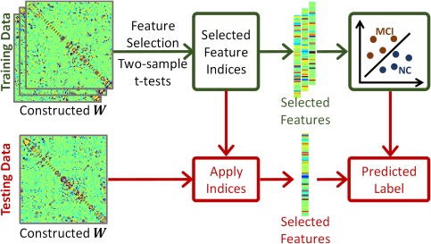
Procedure for mild cognitive impairment (MCI) classification. In the training stage, we use the two‐sample t‐test to select significant features for two classes, i.e., mild cognitive impairment (MCI) and normal control (NC) classes. The selected features will be used to train the classifier. For the testing data, we use the same selected features as used in the training stage to predict the label of testing data as MCI or NC, using the trained classifier. [Color figure can be viewed at http://wileyonlinelibrary.com]
EXPERIMENTS
Subjects and Data
The Alzheimer's Disease Neuroimaging Initiative (ADNI) dataset (Jack et al., 2008) is used in this study. Specifically, 50 MCI patients and 49 NCs are selected from the ADNI‐2 dataset in our experiments. This study has been performed in accordance with the ethical standards as laid down in the 1964 Declaration of Helsinki and its later amendments. Informed consent was obtained from all individual participants included in the study. Subjects from both classes are age‐ and gender‐matched, and they were all scanned using 3.0 T Philips scanners. For details of imaging parameters, please check adni.loni.ucla.edu. In preprocessing, SPM8 toolbox (http://www.fil.ion.ucl.ac.uk/spm/) is used to preprocess the rs‐fMRI data according to the well‐accepted pipeline (Rubinov and Sporns, 2010). Specifically, the first 3 volumes of each subject are discarded before preprocessing for magnetization equilibrium. Then, rigid‐body registration is used to correct head motion (but the subjects with overall head motion larger than 2 mm or 2° during scanning are discarded). The fMRI images are normalized to the Montreal Neurological Institute (MNI) space and spatially smoothed with a Gaussian kernel with full‐width‐at‐half‐maximum (FWHM) of 6 × 6 × 6 mm3. To reduce the negative effect on brain network modeling caused by excessive framewise head motion, we estimate framewise head motion and exclude subjects who have too many frames with excessive framewise head motion. Specifically, we calculate framewise displacement (FD) based on Power et al.'s (2011) algorithm and exclude the subjects with more than 2.5 min (50 frames) data of FD > 0.5 from further analysis (Wu et al., 2015). However, we do not censor the data of the remaining subjects to ensure them to have the equal number of rs‐fMRI data, to make the functional connectivity network modeling results comparable across subjects. Head motion parameters (i.e., Friston‐24 model) and the mean BOLD time series of white matter and cerebrospinal fluid are regressed out from the band‐pass filtered (0.01–0.08 Hz) rs‐fMRI data.
Brain Functional Network Construction
For each subject, the mean rs‐fMRI signals extracted from N = 90 ROIs defined by Automated Anatomical Labeling (AAL) template (Tzourio‐Mazoyer et al., 2002) are utilized to model brain functional network. For comparison, we also construct brain networks using two basic methods, PC and SR. To further explore the effects of both the proposed connectivity strength‐based weighting and structure‐grouping, we have also compared our proposed WSGR with both SGR (without weight ) and WSR (without group constraint). Their matrix‐regularized objective functions are provided in Table 1.
Table 1.
Brain functional network construction models
| Method | Data‐fitting term | Regularization term | ||
|---|---|---|---|---|
| PC |
|
— | ||
| SR |
|
|
||
| WSR |
|
|
||
| SGR |
|
|
||
| WSGR |
|
|
Note: The regularized parameters , are positive; .
PC, Pearson's correlation; SR, sparse representation; SGR, sparse group representation; WSR, weighted sparse representation; WSGR, weighted sparse group representation.
The optimization of the objective functions of the SGR and WSGR models can be solved by the Moreau–Yosida regularization associated with the sparse group Lasso penalty (Liu and Ye, 2010). All the SR models in this article are solved using SLEP toolbox (Liu et al., 2009), and is initialized with zero matrix.
Figure 5 shows the visualization of the constructed brain functional networks from a randomly selected subject using five different methods separately. As can be seen from Figure 5a, the intrinsic grouping in brain connectivity is observed, whereas the PC‐based brain network is very dense. All the networks constructed from the SR models are sparse. Regarding the effectiveness of using the connectivity strength‐based weights, we can see that the sparse constraint with the connectivity strength‐based weights (Figure 5d,e) is more reasonable in modeling brain functional network than its counterparts without weights (Figure 5b,c). Compared with the traditional SR models, some connections with high connectivity strength are enhanced by the WSR models, and vice versa. This validates the effectiveness of our proposed method which integrates the pairwise correlation and the sparse learning. Regarding the grouping constraint used, the group structure is more obvious in Figure 5e by our WSGR method than in Figure 5d by WSR.
Figure 5.
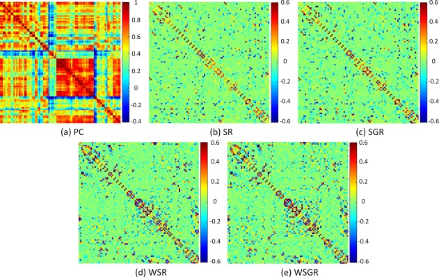
Comparison of brain functional networks of the same subject, reconstructed by five different methods, based on (a) Pearson's correlation (PC), (b) sparse representation (SR), (c) sparse group representation (SGR), (d) weighted sparse representation (WSR), and (e) weighted sparse group representation (WSGR). [Color figure can be viewed at http://wileyonlinelibrary.com]
Classification Results
After constructing the brain functional networks, we regard the connections as features for MCI classification. A leave‐one‐out cross‐validation (LOOCV) strategy is adopted in our experiments. To set the values of the regularization parameter (i.e., λ in SR and WSR, and λ 1, λ 2 in SGR and WSGR), we employ a nested LOOCV strategy on the training set to grid‐search the respective parameter values in the range of .
Specifically, given a total of subjects, one of them is left out for testing, and the remaining −1 subjects are used for training. Then, we select the optimal parameter values by grid‐searching on the training set with the nested LOOCV strategy. Specifically, among these −1 subjects, a training subset with −2 subjects was formed by leaving one training subject out to test in the nested LOOCV procedure (based on the t‐test with default p < 0.05 for feature selection, and the linear SVM with default c = 1 for classification). Thus, there are −1 different training subsets and −1 corresponding testing samples. The combination of regularization parameters that gives the best performance is selected as the optimal parameters. Then, by backing to the training set with −1 subjects, we apply the optimal regularization parameters onto the −1 different training subsets, each with −2 subjects. Note, there are −1 classifiers that are used to classify the completely unseen testing subject. The final classification decision is determined via majority voting. Every subject in the whole dataset will be left out for testing, so the above process repeats S times. Finally, an overall cross‐validation classification accuracy is calculated.
To evaluate the classification performance, we use seven evaluation measures: accuracy (ACC), sensitivity (SEN), specificity (SPE), area under curve (AUC), Youden's index (YI), F‐score, and balanced accuracy (BAC). The detailed definitions of these seven statistical measures except area under ROC curve (AUC) are provided in Table 2, where TP, TN, FP, and FN denote the true positive, true negative, false positive, and false negative, respectively, and and . In this article, we treat the MCI samples as positive class and the NC samples as negative class.
Table 2.
Definitions of six statistical measurement indices
| Measurement | Definition | |
|---|---|---|
| ACC |
|
|
| SEN |
|
|
| SPE |
|
|
| YI |
|
|
| F‐Score |
|
|
| BAC |
|
ACC, accuracy; SEN, sensitivity; SPE, specificity; YI, Youden's index; BAC, balanced accuracy.
As shown in Figure 6, the proposed brain network construction model (using weighted group sparsity) achieves the best classification performance with an accuracy of 84.85%, followed by WSR with an accuracy of 79.80%. By comparing these results, we can verify the effectiveness of connectivity strength‐based weights from two aspects. First, it can be observed that the WSR model with connectivity strength‐based weights performs much better than PC and SR models. Second, the classification result of the WSGR model outperforms the SGR model (with an accuracy of 72.73%). Similarly, by comparing the results of the SR and WSR models with those of the SGR and WSGR models, the effectiveness of our introduced group structure‐based penalty can be well justified. The superior performance of our method suggests that the weighted group sparsity is beneficial in constructing brain networks and is also able to improve classification performance. Figure 6b shows the ROC curves of different methods. To further confirm the statistical significance of classification results by different methods, we adopt the DeLong's (1988) test, which allows for the comparison of two ROC curves calculated on the dataset, by performing a nonparametric statistical test. The results show that our proposed WSGR significantly outperforms PC, SR, WSR, and SGR under 95% confidence interval with p values and respectively.
Figure 6.

Comparison of classification results by five different methods using 7 performance metrics and also ROC curves. Results are based on the Pearson's correlation (PC), sparse representation (SR), sparse group representation (SGR), weighted sparse representation (WSR), and weighted sparse group representation (WSGR). Seven metrics include accuracy (ACC), sensitivity (SEN), specificity (SPE), area under curve (AUC), Youden's index (YI), F‐Score, and balanced accuracy (BAC). [Color figure can be viewed at http://wileyonlinelibrary.com]
DISCUSSIONS
Top Discriminative Features
As the selected features by two‐sample t tests in each validation might be different, we record all the selected features during the training process. There are 47 features that are consistently selected in all validations, as visualized in Figure 7, where the red arcs represent the features related to the default mode network (DMN) that have been commonly regarded as AD‐pathology related (Greicius et al., 2004; Teipel et al., 2015). According to previous studies (Fair et al., 2008; Fox et al., 2005), the detailed names for the ROIs related with DMN are listed in the Table I in Supporting Information. Interestingly, most of these consistently selected discriminative features are the DMN‐related connectivities. The grey arcs in Figure 7 denote the consistently selected discriminative features outside the DMN, including the olfactory cortices, middle orbitofrontal cortices, fusiform, caudate, and so on.
Figure 7.
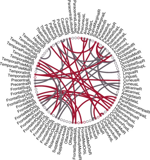
Illustration of 47 consistently selected features (i.e., connections). The red arcs represent the features related to the default mode network. [Color figure can be viewed at http://wileyonlinelibrary.com]
The linear SVM classification model obtained on the training data in each cross‐validation is a maximum‐margin hyperplane, represented by the learned weight coefficients for all selected features. To further study the connectivity pattern that contributed to MCI identification, we average the weight coefficients of each selected feature across all the cross‐validations to analyze the linear classification model. All consistently selected connectivities shown in Figure 7 are displayed in Figure 8 in the full brain view (see also Table II in Supporting Information for detailed connections). Specifically, the nodes here represent the ROIs, with their sizes indicating the sum of weights connecting to each ROI (which can be regarded as the degree of the nodes in the brain network), and the edges represent the connections (or features used in this article) with their thickness indicating the corresponding weights in classification pattern.
Figure 8.
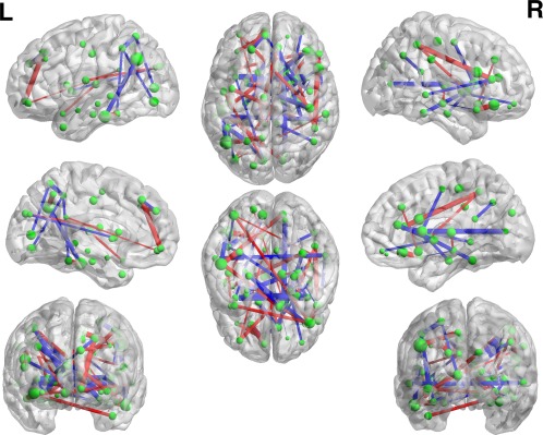
Classification Pattern. The thickness of each edge indicates its weight used in a linear SVM model for MCI classification. [Color figure can be viewed at http://wileyonlinelibrary.com]
The 11 discriminative regions, which have at least three connection features among all the consistently selected features, are shown in Figure 9. Specifically, the right inferior orbitofrontal cortex and right olfactory cortex are highly related to AD pathology, according to previous studies (Tekin and Cummings, 2002). The left superior medial frontal cortex, right anterior cingulate cortex, left inferior parietal lobule, and left inferior temporal gyrus are within the DMN. The right caudate, right putamen, and right pallidum are subcortical regions with dense connections to the cortex, which are important for MCI classification (Albert et al., 2011).
Figure 9.
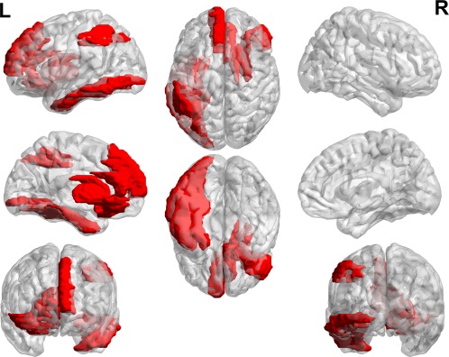
Demonstration of the discriminative regions used in classification. The regions shown in red, i.e., right inferior orbitofrontal cortex, right olfactory cortex, left superior medial frontal cortex, right anterior cingulate cortex, left inferior occipital gyrus, left fusiform gyrus, left inferior parietal lobule, right caudate, right putamen, right pallidum, and left inferior temporal gyrus, have at least three connections as selected features over all the consistently selected features. [Color figure can be viewed at http://wileyonlinelibrary.com]
Sensitivity to Network Model Parameters
To investigate the sensitivity of our model to the involved regularization parameters, i.e., and , we have also conducted an experiment that discards the nested LOOCV parameter selection on the training set. We directly compute the classification accuracy under different parameter combinations in the proposed WSGR method with LOOCV. The classification accuracies are shown in Figure 10. It can be observed that the results change with different values of the regularized parameters, and the best accuracy (87.88%) is achieved with for (weighted) sparsity and for group sparsity. Note that to validate the effectiveness of our proposed method, we adopt the grid‐searching strategy to select the optimal regularization parameters within the training data, while leaving the testing data for validation. The optimal parameters selected automatically in different validations are not fixed. The performance of our method with such grid‐searching strategy achieves 84.85% accuracy, which is close to the highest accuracy 87.88% with specific parameter values.
Figure 10.
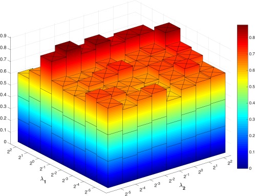
Classification accuracy based on the networks estimated by the proposed method with different regularized parametric values. The parameters are chosen between [ ]. The results are obtained by LOOCV on all subjects. [Color figure can be viewed at http://wileyonlinelibrary.com]
Related Works
In this work, we proposed the connectivity strength‐WSGR model for constructing the brain functional network. In terms of the ‐norm regularization term, it is not only for statistical estimation but also for providing a principled way of incorporating sparsity priors (as brain region predominantly interacts with only a small number of other regions) into a network learning framework. Many neuroscience studies have already suggested that the brain network is sparse (Sporns, 2011). For the group sparsity by ‐norm, there are some similar models on the network construction in the literature. For example, Varoquaux et al. (2010) used group sparsity prior ( ‐norm regularizer) to constrain all subjects within the same group to share the same network topology. Wee et al. (2014) used the similar group‐constrained sparsity to overcome intersubject variability in the brain network construction. In their works, each ROI's representation was still independent to each other, and they did not consider the connectivity strength during the SR.
In terms of combining ‐norm constraint with ‐norm constraint, a recent work (Jiang et al., 2015) defined “group” based on the anatomical connectivity using diffusion tensor imaging, and then applied SGR to construct brain functional network using whole‐brain rs‐fMRI signals. Compared with their work, our method proposes to define the group by using the intrinsic connectivity strength derived from the rs‐fMRI data, which does not need any additional imaging data that sometimes may not be available. In addition, we have added connectivity strength‐based weights to the ‐norm constraint, for constructing more reasonable brain functional network.
CONCLUSION
In this article, we have proposed a novel method with WSGR to optimally construct brain functional network from rs‐fMRI data. We have taken the advantage of both Pearson's correlation and SRs, which are the two most used brain network modeling approaches, to ensure the construction of more biologically meaningful brain network by a unified framework that integrates connectivity strength, group structure, and sparsity. Our proposed method has been validated in the task of MCI and NC classification, obtaining superior results compared to other brain network construction approaches. In future, we plan to work on more effective grouping strategy, i.e., partitioning the links into the overlapping groups, to model more meaningful brain networks. Moreover, our method can be applied to various brain disorders and diseases, such as autism and Parkinson's disease.
Supporting information
Supporting Information
REFERENCES
- Albert MS, DeKosky ST, Dickson D, Dubois B, Feldman HH, Fox NC, Gamst A, Holtzman DM, Jagust WJ, Petersen RC (2011): The diagnosis of mild cognitive impairment due to Alzheimer's disease: Recommendations from the National Institute on Aging‐Alzheimer's Association workgroups on diagnostic guidelines for Alzheimer's disease. Alzheimers Dement 7:270–279. [DOI] [PMC free article] [PubMed] [Google Scholar]
- Chang C‐C, Lin C‐J (2011): LIBSVM: A library for support vector machines. ACM Trans Intell Syst Technol 2:27. [Google Scholar]
- Chen X, Zhang H, Gao Y, Wee CY, Li G, Shen D (2016): High‐order resting‐state functional connectivity network for MCI classification. Hum Brain Mapp 37:3282–3296. [DOI] [PMC free article] [PubMed] [Google Scholar]
- Craddock RC, James GA, Holtzheimer PE, Hu XP, Mayberg HS (2012): A whole brain fMRI atlas generated via spatially constrained spectral clustering. Hum Brain Mapp 33:1914–1928. [DOI] [PMC free article] [PubMed] [Google Scholar]
- Eguiluz VM, Chialvo DR, Cecchi GA, Baliki M, Apkarian AV (2005): Scale‐free brain functional networks. Phys Rev Lett 94:018102. [DOI] [PubMed] [Google Scholar]
- Elhamifar E, Vidal R (2013): Sparse subspace clustering: Algorithm, theory, and applications. IEEE T Pattern Anal 35:2765–2781. [DOI] [PubMed] [Google Scholar]
- Fair DA, Cohen AL, Dosenbach NU, Church JA, Miezin FM, Barch DM, Raichle ME, Petersen SE, Schlaggar BL (2008): The maturing architecture of the brain's default network. Proc Natl Acad Sci 105:4028–4032. [DOI] [PMC free article] [PubMed] [Google Scholar]
- Fornito A, Zalesky A, Breakspear M (2015): The connectomics of brain disorders. Nat Rev Neurosci 16:159–172. [DOI] [PubMed] [Google Scholar]
- Fox MD, Raichle ME (2007): Spontaneous fluctuations in brain activity observed with functional magnetic resonance imaging. Nat Rev Neurosci 8:700–711. [DOI] [PubMed] [Google Scholar]
- Fox MD, Snyder AZ, Vincent JL, Corbetta M, Van Essen DC, Raichle ME (2005): The human brain is intrinsically organized into dynamic, anticorrelated functional networks. Proc Natl Acad Sci USA 102:9673–9678. [DOI] [PMC free article] [PubMed] [Google Scholar]
- Fransson P (2005): Spontaneous low‐frequency BOLD signal fluctuations: An fMRI investigation of the resting‐state default mode of brain function hypothesis. Hum Brain Mapp 26:15–29. [DOI] [PMC free article] [PubMed] [Google Scholar]
- Fransson P, Marrelec G (2008): The precuneus/posterior cingulate cortex plays a pivotal role in the default mode network: Evidence from a partial correlation network analysis. NeuroImage 42:1178–1184. [DOI] [PubMed] [Google Scholar]
- Friedman J, Hastie T, Tibshirani R (2008): Sparse inverse covariance estimation with the graphical lasso. Biostatistics 9:432–441. [DOI] [PMC free article] [PubMed] [Google Scholar]
- Friston K, Frith C, Liddle P, Frackowiak R (1993): Functional connectivity: The principal‐component analysis of large (PET) data sets. J Cereb Blood Flow Metab 13:5–14. [DOI] [PubMed] [Google Scholar]
- Gauthier S, Reisberg B, Zaudig M, Petersen RC, Ritchie K, Broich K, Belleville S, Brodaty H, Bennett D, Chertkow H (2006): Mild cognitive impairment. Lancet 367:1262–1270. [DOI] [PubMed] [Google Scholar]
- Greicius M (2008): Resting‐state functional connectivity in neuropsychiatric disorders. Curr Opin Neurol 21:424–430. [DOI] [PubMed] [Google Scholar]
- Greicius MD, Srivastava G, Reiss AL, Menon V (2004): Default‐mode network activity distinguishes Alzheimer's disease from healthy aging: Evidence from functional MRI. Proc Natl Acad Sci USA 101:4637–4642. [DOI] [PMC free article] [PubMed] [Google Scholar]
- Hampson M, Peterson BS, Skudlarski P, Gatenby JC, Gore JC (2002): Detection of functional connectivity using temporal correlations in MR images. Hum Brain Mapp 15:247–262. [DOI] [PMC free article] [PubMed] [Google Scholar]
- Huang S, Li J, Sun L, Liu J, Wu T, Chen K, Fleisher A, Reiman E, Ye J (2009): Learning brain connectivity of Alzheimer's disease from neuroimaging data. Adv Neural Inf Process Syst. pp. 808–816. [Google Scholar]
- Huang S, Li J, Sun L, Ye J, Fleisher A, Wu T, Chen K, Reiman E, Initiative AsDN (2010): Learning brain connectivity of Alzheimer's disease by sparse inverse covariance estimation. NeuroImage 50:935–949. [DOI] [PMC free article] [PubMed] [Google Scholar]
- Jack CR, Bernstein MA, Fox NC, Thompson P, Alexander G, Harvey D, Borowski B, Britson PJ, L Whitwell J, Ward C (2008): The Alzheimer's disease neuroimaging initiative (ADNI): MRI methods. J Magn Reson Imag 27:685–691. [DOI] [PMC free article] [PubMed] [Google Scholar]
- Jiang X, Zhang T, Zhao Q, Lu J, Guo L, Liu T (2015): Fiber Connection Pattern‐Guided Structured Sparse Representation of Whole‐Brain fMRI Signals for Functional Network Inference. Medical Image Computing and Computer‐Assisted Intervention–MICCAI 2015. Springer; pp 133–141. [Google Scholar]
- Lee H, Lee DS, Kang H, Kim BN, Chung MK (2011): Sparse brain network recovery under compressed sensing. Med Imag IEEE Trans 30:1154–1165. [DOI] [PubMed] [Google Scholar]
- Liu J, Ji S, Ye J (2009): SLEP: Sparse learning with efficient projections. Arizona State Univ 6:491. [Google Scholar]
- Liu J, Ye J (2010): Moreau‐Yosida regularization for grouped tree structure learning. Adv Neural Inf Process Syst. pp 1459–1467. [Google Scholar]
- Meinshausen N, Bühlmann P (2006): High‐dimensional graphs and variable selection with the lasso. Ann Stat 1436–1462. [Google Scholar]
- Peng J, Wang P, Zhou N, Zhu J (2009): Partial correlation estimation by joint sparse regression models. J Am Stat Assoc 104:735–746. [DOI] [PMC free article] [PubMed] [Google Scholar]
- Petersen RC, Doody R, Kurz A, Mohs RC, Morris JC, Rabins PV, Ritchie K, Rossor M, Thal L, Winblad B (2001): Current concepts in mild cognitive impairment. Arch Neurol 58:1985–1992. [DOI] [PubMed] [Google Scholar]
- Power JD, Cohen AL, Nelson SM, Wig GS, Barnes KA, Church JA, Vogel AC, Laumann TO, Miezin FM, Schlaggar BL (2011): Functional network organization of the human brain. Neuron 72:665–678. [DOI] [PMC free article] [PubMed] [Google Scholar]
- Rombouts SA, Barkhof F, Goekoop R, Stam CJ, Scheltens P (2005): Altered resting state networks in mild cognitive impairment and mild Alzheimer's disease: An fMRI study. Hum Brain Mapp 26:231–239. [DOI] [PMC free article] [PubMed] [Google Scholar]
- Rosa MJ, Portugal L, Hahn T, Fallgatter AJ, Garrido MI, Shawe‐Taylor J, Mourao‐Miranda J (2015): Sparse network‐based models for patient classification using fMRI. NeuroImage 105:493–506. [DOI] [PMC free article] [PubMed] [Google Scholar]
- Rubinov M, Sporns O (2010): Complex network measures of brain connectivity: Uses and interpretations. NeuroImage 52:1059–1069. [DOI] [PubMed] [Google Scholar]
- Salvador R, Suckling J, Coleman MR, Pickard JD, Menon D, Bullmore E (2005): Neurophysiological architecture of functional magnetic resonance images of human brain. Cereb Cortex 15:1332–1342. [DOI] [PubMed] [Google Scholar]
- Simon N, Friedman J, Hastie T, Tibshirani R (2013): A sparse‐group lasso. J Comput Graph Stat 22:231–245. [Google Scholar]
- Smith SM, Miller KL, Salimi‐Khorshidi G, Webster M, Beckmann CF, Nichols TE, Ramsey JD, Woolrich MW (2011): Network modelling methods for FMRI. NeuroImage 54:875–891. [DOI] [PubMed] [Google Scholar]
- Sorg C, Riedl V, Mühlau M, Calhoun VD, Eichele T, Läer L, Drzezga A, Förstl H, Kurz A, Zimmer C (2007): Selective changes of resting‐state networks in individuals at risk for Alzheimer's disease. Proc Natl Acad Sci 104:18760–18765. [DOI] [PMC free article] [PubMed] [Google Scholar]
- Sporns O (2011): Networks of the Brain. Cambridge, MA: MIT Press. [Google Scholar]
- Sporns O, Chialvo DR, Kaiser M, Hilgetag CC (2004): Organization, development and function of complex brain networks. Trends Cogn Sci 8:418–425. [DOI] [PubMed] [Google Scholar]
- Supekar K, Menon V, Rubin D, Musen M, Greicius MD (2008): Network analysis of intrinsic functional brain connectivity in Alzheimer's disease. PLoS Comput Biol 4:e1000100. [DOI] [PMC free article] [PubMed] [Google Scholar]
- Teipel S, Drzezga A, Grothe MJ, Barthel H, Chételat G, Schuff N, Skudlarski P, Cavedo E, Frisoni GB, Hoffmann W (2015): Multimodal imaging in Alzheimer's disease: Validity and usefulness for early detection. Lancet Neurol 14:1037–1053. [DOI] [PubMed] [Google Scholar]
- Tekin S, Cummings JL (2002): Frontal–subcortical neuronal circuits and clinical neuropsychiatry: An update. J Psychosomatic Res 53:647–654. [DOI] [PubMed] [Google Scholar]
- Tzourio‐Mazoyer N, Landeau B, Papathanassiou D, Crivello F, Etard O, Delcroix N, Mazoyer B, Joliot M (2002): Automated anatomical labeling of activations in SPM using a macroscopic anatomical parcellation of the MNI MRI single‐subject brain. NeuroImage 15:273–289. [DOI] [PubMed] [Google Scholar]
- Van Den Heuvel MP, Pol HEH (2010): Exploring the brain network: A review on resting‐state fMRI functional connectivity. Eur Neuropsychopharmacol 20:519–534. [DOI] [PubMed] [Google Scholar]
- Varoquaux G, Gramfort A, Poline J‐B, Thirion B (2010): Brain covariance selection: Better individual functional connectivity models using population prior. Adv Neural Inf Process Syst. pp 2334–2342. [Google Scholar]
- Wang K, Liang M, Wang L, Tian L, Zhang X, Li K, Jiang T (2007): Altered functional connectivity in early Alzheimer's disease: A resting‐state fMRI study. Hum Brain Mapp 28:967–978. [DOI] [PMC free article] [PubMed] [Google Scholar]
- Wee CY, Yap PT, Denny K, Browndyke JN, Potter GG, Welsh‐Bohmer KA, Wang L, Shen D (2012): Resting‐state multi‐spectrum functional connectivity networks for identification of MCI patients. PLoS One 7:e37828. [DOI] [PMC free article] [PubMed] [Google Scholar]
- Wee CY, Yap PT, Zhang D, Wang L, Shen D (2014): Group‐constrained sparse fMRI connectivity modeling for mild cognitive impairment identification. Brain Struct Funct 219:641–656. [DOI] [PMC free article] [PubMed] [Google Scholar]
- Wernick MN, Yang Y, Brankov JG, Yourganov G, Strother SC (2010): Machine learning in medical imaging. IEEE Signal Process Magaz 27:25–38. [DOI] [PMC free article] [PubMed] [Google Scholar]
- Wu X, Zou Q, Hu J, Tang W, Mao Y, Gao L, Zhu J, Jin Y, Wu X, Lu L (2015): Intrinsic functional connectivity patterns predict consciousness level and recovery outcome in acquired brain injury. J Neurosci 35:12932–12946. [DOI] [PMC free article] [PubMed] [Google Scholar]
- Yuan M, Lin Y (2006): Model selection and estimation in regression with grouped variables. J Royal Stat Soc Ser B Stat Methodol 68:49–67. [Google Scholar]
Associated Data
This section collects any data citations, data availability statements, or supplementary materials included in this article.
Supplementary Materials
Supporting Information


