Anatomy-guided lung lobe segmentation in X-ray CT images

Abstract

The human lungs are divided into five distinct anatomic compartments called the lobes, which are separated by the pulmonary fissures. The accurate identification of the fissures is of increasing importance in the early detection of pathologies, and in the regional functional analysis of the lungs. We have developed an automatic method for the segmentation and analysis of the fissures, based on the information provided by the segmentation and analysis of the airway and vascular trees. This information is used to provide a close initial approximation to the fissures, using a watershed transform on a distance map of the vasculature. In a further refinement step, this estimate is used to construct a region of interest (ROI) encompassing the fissures. The ROI is enhanced using a ridgeness measure, which is followed by a 3-D graph search to find the optimal surface within the ROI. We have also developed an automatic method to detect incomplete fissures, using a fast-marching based segmentation of a projection of the optimal surface. The detected incomplete fissure is used to extrapolate and smoothly complete the fissure. We evaluate the method by testing on data sets from normal subjects and subjects with mild to moderate emphysema.

I. Introduction

THE human lungs are divided into five distinct anatomic compartments called lobes. The separating junctions between the lobes are called the lobar fissures. The left lung consists of the upper and lower lobes, which are separated by the left oblique or major fissure. The right lung consists of the upper, middle, and lower lobes: the upper and middle lobes are separated by the horizontal or minor fissure; the middle and upper lobes and separated from the lower lobe by the right oblique (major) fissure. It has been hypothesized that the fissures allow the lobes to rotate relative to one another to accommodate shape changes in the thoracic cavity [1], [2]. The branching patterns of the airway and vascular trees are closely related to the lobar anatomy. Although there are some exceptions, mainly in the case of incomplete fissures, each lobe is served by separate airway and vascular networks.

Some pulmonary diseases are more prevalent in specific anatomic regions of the lung. For example, tuberculosis and silicosis are almost exclusively upper lobe diseases, while interstitial pulmonary fibrosis is more commonly present in the lower lobes. Pulmonary emphysema is commonly more severe in the upper lobes, but there is a rare genetic variant associated with alpha–1 anti-trypsin deficiency that is prevalent in the lower lobes. Thus, segmentation of the lobes and understanding the tissue and functional characteristics of the lobar parenchyma is clinically important for disease classification and may provide insights into the basic pathophysiology of lung disease.

Treatment selection, planning, and followup may also benefit from lobar analysis. For example, there are emerging therapies for emphysema that use full lobar exclusion via one-way valves implanted into the airways. These therapies rely on identifying the airway and lobar distribution in CT images. In addition, it may be important to identify incomplete fissures, as it is believed that incomplete fissures may allow collateral ventilation between lobes that may compromise the lobar exclusion.

CT imaging can be used to study the lobar anatomy. A major challenge to the automatic detection of the fissures is the fact that the fissures have low contrast and variable shape and appearance in CT imagery, which sometimes makes it difficult even for manual analysts to mark their exact location. Usually, the fissures appear as a thin bright sheet, dividing the lung parenchyma into two parts (see Figure 1). But, as has been shown by Hayashi et al. [9], some pulmonary diseases can alter the appearance of the fissures on CT images. Also, for a significant fraction of datasets, a phenomenon called fissure disintegration is observed — fissure disintegration is the absence of the fissures at their expected location, leading to incomplete fissures (see Figure 1(a)).

Fig. 1.

(a) Sagittal slice from the right lung showing the right oblique and horizontal fissures — the horizontal fissure is oriented horizontally, while the oblique fissure is tilted away from the vertical axis, (b) sagittal slice from the left lung showing the left oblique fissure, (c) transverse slice from a different data set that shows an incomplete right oblique fissure.

Table I summarizes recent CT-based lobe segmentation studies. Previous approaches to lobe segmentation can be roughly divided into two classes: direct and indirect. The former approaches consist of methods that search for the fissures based on gray-level information present in the data, while the latter approaches consist of methods that use information from other anatomical structures to approximate the location of the fissures. Of the direct methods, Zhang et al. [4] presented a method for automatic segmentation of the oblique fissures using an atlas-based initialization procedure, followed by a two-step graph searching procedure to delineate the fissures. One drawback of the atlas-based initialization is the time-intensive atlas construction, which involves manually delineating the fissures on a number of subjects, and the computationally expensive deformation of the atlas fissures onto a template image. Wang et al. [5], proposed a method for segmentation of the fissures using a 2-D shape-based curve growing model. Their method involves a semi-automatic initialization, after which the oblique fissures are segmented in 2-D slices automatically using a Bayesian formulation influenced by both image data and similarity to a shape prior. Wiemker et al. [6] proposed an automatic segmentation approach based on 3-D filtering of the image data. The Hessian-matrix and structure-tensor based filters are used to enhance the fissures. More recently, van Rikxoort et al. [3] described a nearest-neighbor classifier approach to identifying voxels on the fissures. Since their method identifies fissure voxels, a post-processing step is needed to define a fissure surface separating the lobes.

Table I.

High-resolution CT based studies on automatic lobar fissure segmentation.

Authors	Reported Results	Comments
van Rikxoort et al. [3]	95% classifier accuracy	direct, voxel classifier, needs post-processing steps to define lobar surfaces
Zhang et al. [4]	1.96 mm mean RMS error	direct, atlas-based, computationally intensive, horizontal fissure semi-automatic
Wang et al. [5]	1.01 mm average distance error	direct, shape-based, semi-automatic, oblique fissures only
Wiemker et al. [6]	no validation	direct, 3-D sheet filtering
Kuhnigk et al. [7]	no validation	indirect, watershed transform based, semi-automatic
Zhou et al. [8]	no validation	indirect, Voronoi division based

Among the indirect approaches, Kuhnigk et al. [7], proposed a method for the indirect estimation of the lobes, using information from the segmented vasculature. They presented a method for semi-automatic segmentation of the lobes using a watershed transform on a distance map of the vasculature. Their method required that the user manually place place markers on vessels to guide the segmentation. Their method is fast and interactive, with the ability to edit the results in real time. In a similar approach, Zhou et al. [8] reported a method based on the Voronoi division of the lungs using the lobar bronchi. In the related field of liver segment estimation, Beichel et al. [10] use the vasculature for a nearest-neighbor based partitioning of the liver.

Our approach to the lobar segmentation problem is to use the anatomical information provided by the segmentation and analysis of the airway and vascular trees to guide the segmentation of the fissures. We follow a two-step approach: in the first step an approximate fissure region of interest (ROI) is generated using the airway and vascular trees anatomical information; in a further refinement step, the fissures are accurately located using the available contrast information in the ROI. The algorithm is robust with respect to common variations in scan parameters such as X-ray dosage, lung volume, and CT reconstruction kernels, and has been applied to images of both normal and diseased subjects. We have also developed a fully automatic method to detect incomplete fissures, using a fast-marching based segmentation of a projection of the optimal fissure surface computed by the graph search. Once detected, the incomplete fissure can be used to extrapolate and smoothly complete the fissure surface.

II. Methods - Initial lobe segmentation

A. Overview

Figure 2 shows a flow diagram of the overall process, beginning with the segmentation of the lungs, airways, and vessels. The lungs are segmented from the original image using the automatic method reported in [11]. Airway tree segmentation and branchpoint labeling is done using the methods reported in [12] and [13]. The anatomically labeled airway tree is used to extract the sub-trees corresponding to each of the lobes. The segmented airway tree is then used to smooth the lung contours. The automatic pulmonary vessel segmentation method is based on the algorithm reported in [14]. Next, a distance map is computed on the segmented vasculature. The distance map is combined with the original image to form the input to the watershed transform. The watershed simulation proceeds and the basins are merged using markers automatically generated from the anatomically labeled airway tree. After the watershed analysis is completed, we obtain an approximate segmentation of the lobar fissures.

Fig. 2.

Flow diagram of the fissure segmentation process. First, the lungs, airways, and vessels are detected. Using this anatomic information, an approximate fissure ROI is estimated. This ROI is refined using image grayscale information.

B. Interactive Watershed Transform (IWT)

The watershed transform is an important algorithm for image segmentation. In the watershed transform, a grayscale image is interpreted as a terrain, with the height of each point in the terrain given by its intensity in the grayscale image. In this context, a watershed transform identifies the minima, or basins, in the terrain, and the watersheds, or merges, separating the basins. Vincent et al. [15] presented a fast algorithm for calculating watershed transforms using a simulation of the flooding of the image terrain from below.

Hahn et al. [16] proposed a two-step interactive watershed transform (IWT) based on the original algorithm by Vincent et al. The first, non-interactive step involves a sorting of all image voxels according to intensity, and processing them in the sorted order. A submersion simulation is performed by considering each voxel and its neighbors, and the output is a hierarchical decomposition of the image into basins and merges. In the second step a flooding threshold and manually-selected markers are used to merge the basins. This second step is very fast and can be repeated any number of times to refine the segmentation by adding or deleting markers.

C. Algorithm

The algorithm for an initial estimation of the lobar borders consists of the following main steps:

1. Smoothing of the lung contour: We use a 2-D morphological closing operation with a disk-shaped structuring element with a 2 cm radius on each transverse slice to produce a smooth lung boundary. This is done to fill in the indentations in the lung surface, and to attempt to connect the separate vascular sub-trees for each lobe at the mediastinal border. Figure 3 shows the lung contour on a transverse slice before and after smoothing.

2. Segmentation of pulmonary vessels: A simplified variant of the algorithm proposed by Shikata et al. [14] is used to segment the vessels. Shikata et al. use a two-step approach: a line-filtering of the raw data based on an eigen-analysis of the Hessian matrix calculated at multiple scales (1, √2, 2, 2√2 and 4 voxels), followed by a time-consuming vessel tracking approach to extract the small vessel segments which are missed in the first step. For our purposes the second step is not necessary and is undesirable because of the increased computational cost. In our case, the line-filtered result is thresholded to retain only voxels with line-filtered value less than -0.08, and then subsequently size filtered to remove all segments less than than 75 mm³. Figure 4(a)) shows an example of a vascular tree obtained using this approach.

3. Calculating a modified vessel distance map: As can be seen in Figure 4(a), the fissures are characterized by the sparseness of the vessel tree in the region surrounding them. This can be quantified by computing a distance map of the segmented vasculature, which should a have local maxima along the fissures. The airway segmentation can also included in the distance map computation. However, currently available airway segmentation algorithms are limited in terms of the number of generations segmented. Therefore the additional information gained by using the airways to mark the fissure region the fissures is small. In addition, we would also like to preserve the fissure contrast information that is available in the original image. Following the approach of [7], we create a modified distance map image by combining the distance map and the original image. Let I represent the original CT image data and let A and V represent the image voxels that are identified as airway and vessel voxels during the airway and vessel segmentations. The modified distance map is calculated as follows:

   • Offset the graylevels in the original image I so that the minimum CT value within the lung mask is 0.

   • Find the brightest vessel voxel value, υ_max, within V and the darkest airway voxel value, a_min, within A.

   • Compute a chamfer distance map image, D, on the vessel mask, using the standard 3×3×3 kernel [17]. The distance is computed from every background voxel to the nearest vessel voxel.

   • Create the modified distance map O by combining the distance map image D and original image I:

     $$O_{\upsilon }=\{\begin{array}{cc}{\upsilon }_{\mathit{\text{max}}}-I_{\upsilon }& \text{if}\upsilon \in V;\\ I_{\upsilon }-a_{\mathit{\text{min}}}& \text{if}\upsilon \in A;\\ {\upsilon }_{\mathit{\text{max}}}+I_{\upsilon }+\alpha \ast D_{\upsilon }& \text{otherwise}.\end{array}$$

     where I_υ, O_υ, and D_υ are the voxel values at location υ in the input, output, and chamfer distance map images, and α is the scale factor used to combine the original image and distance map image; in this work we use a value of 10 for α.

   • Using this construction, the airways and vessels are forced to correspond to minima (basins) of the graylevel topography and the fissures are near the watersheds separating these basins from one another. The markers placed on the vessels and airways will flood and fill the corresponding lobe, similar to the rising water analogy of the watershed transform.

4. 3-D watershed transform: We apply the watershed transform to the modified distance map image.

5. Lobar segmentation: The basins generated by the watershed transform are merged according to anatomically-defined markers. The markers for merging can be selected automatically from the anatomically labeled airway tree, and from a priori shape and orientation information about the fissures and the lungs:

6. Using a formal graph description of the airway tree, we extract the sub-tree for a given lobe by doing a breadth-first search from the corresponding lobar root (see Figure 4(b)). Once the sub-trees are extracted, we select the sub-tree centerline points as markers. Selection of markers from the vascular tree is based on the fact that airway and vascular branch segments are located near each other. We construct a 3-D window around each branchpoint of the lobar sub-tree and select all vascular voxels within the window as markers. The window dimensions used in our experiments are given in Table II.

7. Additional markers can also be selected based on a-priori shape information about the fissures. For example, the most apical transverse slices in the data depict tissue that belongs to the upper lobes, so vessel voxels on those slices can be selected as upper lobe markers. On sagittal views, the oblique fissures are oriented at an approximately 45° angle (see Figure 1). We can mark three distinct points along a sagittal contour: the top most point, and the two points of highest curvature in the bottom left corner and the bottom right corner. Based on these 3 points, we compute two lines which divide the lung into distinct upper and lower lobes segments. Vessel voxels lying in these segments are selected as markers for the corresponding lobes. The lines are chosen conservatively, away from the fissure location, so as to not select incorrect seeds and augment the seeds already selected using the airway tree.

Fig. 3.

Lung contour (a) before smoothing, (b) after smoothing.

Fig. 4.

(a) Volume rendered vascular tree showing the relationship between the vascular tree and the lobar boundaries; (b) Anatomically labeled airway tree (from [13]) showing lobar sub-trees. The airway branchpoints TriLUL, LLB6, TriRUL, RB4 + 5 and TriEndBronInt correspond to the left upper lobe, left lower lobe, right upper lobe, right middle lobe and the right lower lobe, respectively.

Table II. Window dimensions (mm) for seed selection for each lobe.

	Xmin	Xmax	Ymin	Ymax	Zmin	Zmax
Left upper	−11.17	5.58	−16.75	2.79	−1.80	0.00
Left lower	−5.58	11.17	−2.79	16.75	0.00	1.80
Right upper	−11.17	11.17	−16.75	8.37	−1.80	0.00
Right middle	−8.37	11.17	−11.17	5.58	−1.80	0.00
Right lower	−5.58	11.17	−2.79	16.75	0.00	1.80

Figures 9(b,e) show the segmented lobes overlaid on sample slices of the original CT data.

Fig. 9.

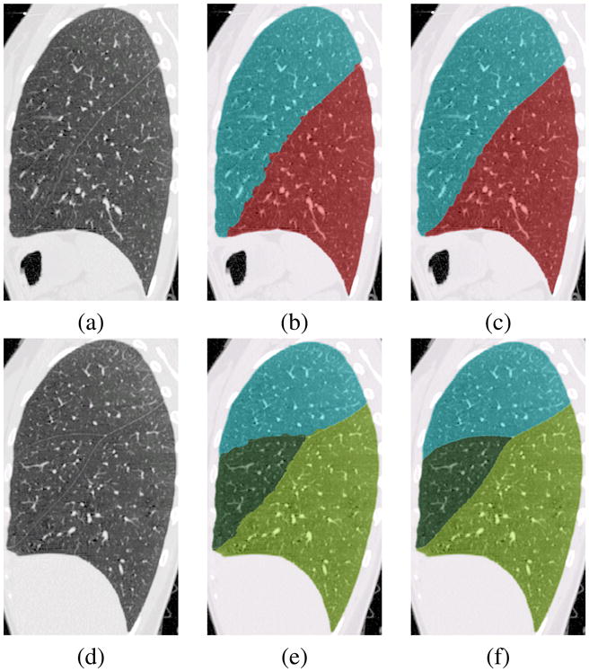
(a,d) CT data, (b,e) Watershed segmentation, (c,f) Optimal surface detection.

In a few instances, the markers selected using the method described above are not sufficient to segment the five lobes, in which case manually selected markers are needed. Figures 5(a,b) show a typical instance where manual editing is usually necessary. As seen in Figure 5(a), a vessel segment which belongs to the left upper lobe has been mislabelled due to its proximity to an airway segment belonging to the left lower lobe. The airway skeleton point within that segment is one of the automatic markers selected for the left lower lobe, which causes the spreading of its label to the adjacent vessels. By placing a single marker on the mislabelled vessel, the segmentation is corrected in this instance, as shown in Figure 5(b).

Fig. 5.

(a) mislabelled vessel in left upper lobe, (b) segmentation after manual interaction.

III. Methods - Fissure Refinement

A. Overview

The initial fissure segmentation described above is primarily based on the distribution of the vasculature rather than on the fissure grayscale information. As shown in Figures 9(b,e), even though the initial lobar border estimates are close to the actual fissure locations, they do not accurately follow the fissures as evinced by their lack of smoothness. This section describes the accurate segmentation of the oblique fissures by optimal surface detection using a 3-D graph search.

B. Optimal Surface Segmentation

In 2-D, optimal path detection using graph searching has been widely used in image segmentation and quantitative analysis. The extension in 3-D is finding the optimal surface through a geometric graph, where each vertex corresponds to a node in the graph. Recently, Wu et al. [18] proposed a polynomial time method for computing globally optimal surfaces in 3-D, using hard smoothness constraints. The problem is modeled as a weighted geometric graph, and the smoothness constraints are hard because they are enforced by the edge connectivity between the vertices. The optimal surface problem was shown to be equivalent to the well-known minimum closed set problem, which can be solved by computing a minimum s – t cut on a derived directed graph. The algorithm has polynomial time complexity. We use the implementation by Li et al. [19] for the fissure refinement.

C. Algorithm: Oblique fissure refinement

The oblique fissure refinement algorithm consists of the following steps:

1. ROI definitions: Three ROIs are defined for the fissure refinement step: ROI₁, ROI₂, and LUNG (see Figure 6). Region ROI₁ consists of all voxels in the lung mask that are a distance d₁ or less from the initial fissure segmentation. Region ROI₂ represents the set of likely fissure endpoints, and consists of all voxels outside the segmented lungs that are a distance d₂ from the initial fissure segmentation. Region LUNG contains all other voxels in the lung mask. d₁ and d₂ are experimentally determined distance thresholds; we use d₁ = 6 mm and d₂ = 4 mm in our work.

2. ROI rotation: To accurately locate the fissures, we find the optimal surface Y_opt = f(x, z) on the graph defined by the bounding-box of ROI₁.Each voxel in the ROI corresponds to a vertex in the graph. It is necessary to keep the graph Y dimension small in order to achieve reasonable runtimes for the graph search algorithm; as discussed in [19], the run-time of the algorithm is proportional to n², where n is the number of vertices in the graph. As shown in Figure 1, the oblique fissure is oriented at approximately 45° relative to the Z (vertical) axis. We estimate this angle by using a least-squares fit of a straight line to the initial fissure segmentation as viewed on the middle sagittal slice. We then rotate the entire image by this angle along an axis parallel to the X axis, and passing through the center of the Y – Z plane of the lung bounding box.

   Tri-linear interpolation is used during the rotation. In addition to rotation, we resample the image data onto an isotropic grid. If x_i, y_i, and z_i are the original voxel dimensions, we define a new grid with voxel dimensions x_o = y_o = z_o = min(x_i, y_i, z_i). There are two advantages to isotropic re-sampling. First, in the case of thick-slice data, in which case z_i may be more than double x_i or y_i, the resampling helps preserve the fissure contrast. Secondly, as described in Section VI-B, by increasing the resampled voxel size we can reduce the overall graph search runtime by reducing the graph size.

   After rotation and resampling, we find the bounding-box for the label ROI₁, as shown in Figure 8(a). The voxels of the bounding box define the vertices of the graph G, within which the optimal surface is computed.

3. Calculating the ridgeness map: On transverse slices the oblique fissure appears like a ridge in the gray-level topography of the lungs. To enhance the ridges and valleys in the image, we use the method MLSEC-ST (multilocal level set extrinsic curvature and its enhancement by structure tensors) [20]. It is a multilocal approach, based on eigen-analysis of the structure tensor. The eigenvector corresponding to the largest eigenvalue correspond to the dominant gradient vector in the neighborhood. Ridges are enhanced by using the difference in the eigenvalues, which is a measure of anisotropy. In this work, the gradients are calculated by convolution with a Gaussian of width 2 voxels, and a Gaussian of width 5 voxels was used for the structure tensor calculations. In addition, we note that the orientation of the eigenvectors around a ridge provides an estimate of the orientation of the ridge. Therefore, using a priori knowledge about orientation of the structures which are being enhanced, an orientation sensitivity term D was included into the measure proposed by Lopez et al. [20]:

   $$D(x,y)=e^{-{\left(O\right(x,y)-\theta )}^2}/2d^2,$$

   where θ is the estimated mean direction, O(x, y) is the direction of the eigenvector, and d is the standard deviation of the Gaussian distribution. Our implementation uses θ = 75° and d = 0.4. For computational efficiency we calculate the ridgeness map over all transverse (X – Y) slices; however a 3-D ridgeness calculation is also possible. Figure 8(b) shows a sample sagittal slice from the ridgeness map.

4. Calculating the cost function: The cost function image C used for computing the optimal surface is based on the ridgeness map, and is defined as follows:

   $$C_{\upsilon }=\{\begin{array}{cc}-(I_{\upsilon }+R_{\upsilon })& \text{if}\upsilon \in {\text{ROI}}_1;\\ C_1& \text{if}\upsilon \in {\text{ROI}}_2;\\ C_2& \text{if}\upsilon \in \text{LUNG};\\ C_3& \text{otherwise}.\end{array}$$

   where C_υ, I_υ, and R_υ are the cost function image, the original CT image, and the ridgeness image at voxel location υ. The ridgeness map is scaled to be of the same range as the CT image. Constants C₂ and C₃ are set to very high values to keep the search within the fissure ROI and C₁ is set to a smaller value to cause a smooth transition of the optimal surface from the inside of the lung to the outside of the lung. In our work we use C₁ = 100, C₂ = 2000, and C₃ = 1000.

5. Optimal surface calculation: We compute the optimal 3-D surface Y_opt = f(x, z) within the graph G with vertex weights defined by the cost function image C. The algorithm proposed by Wu et al. [18] is used to calculate the optimal surface.

   The optimal surface is a single voxel wide surface dividing the lung, while our final objective is to generate a labeled volume with separate labels for the upper and lower lobes. We use a fast breadth-first region growing technique as proposed by Silvela et al. [21] to grow and label the upper and lower lobar regions. Then the labels are rotated back to the original orientation using nearest neighbor interpolation.

   Figures 9(c,f) show the results from the optimal surface graph search, based on the ROIs defined by the watershed segmentation results shown in Figures 9(b,e).

Fig. 6.

Fissure ROI for left oblique fissure.

Fig. 8.

Sagittal plane from bounding box showing (a) Rotated ROI, (b) Ridgeness map.

D. Algorithm: Horizontal fissure refinement

After performing the segmentation and refinement for the right oblique fissure, the right lung is divided into two components: the right lower lobe and the combined right upper and middle lobes. To refine the segmentation of the horizontal fissure, we find the optimal surface Z_opt = f(x, y), which divides the combined right upper plus right middle lobes into separate upper and middle lobes. The steps for finding the optimal surface corresponding to the horizontal fissure are similar to those for refining the oblique fissures. For most cases the angle that the horizontal fissure makes with the X – Y plane is small, and hence the Z dimension of the ROI bounding box is small enough so that a reasonable runtime is possible without rotation. We do, however, perform resampling to make the voxels isotropic. For the horizontal fissure we calculate the ridgeness measure on sagittal (Y – Z) slices of the image data because the ridge-like nature of the horizontal fissure is most evident on sagittal slices (see Figure 1(a)).

Figure 9(f) shows the segmented middle lobe resulting from the optimal surface graph-search for the horizontal fissure. This result is based on the ROI defined by the watershed segmentation result shown in Figure 9(e).

IV. Methods -Incomplete fissure detection and fissure smoothing

A. Introduction

As mentioned in the introduction, there is interest in detecting and measuring incomplete fissures. Figure 1(c) shows a case with an apparent incomplete fissure. In this example, the fissure appears to be missing at some locations in the image, either due to the anatomic structure of the lobes or because of limitations in the imaging system. Our observations have been that incomplete fissures always occur on the mediastinal side of the fissure. The incompleteness of the fissure is accompanied by a fusion of the lung parenchyma from the adjacent lobes. As pointed out by Hayashi et al. [9], studies differ as to the how often the fissure is incomplete. Our own experience has been that in about 30-40% of the cases the major fissures appear incomplete, with an increased prevalence for incompleteness in the right oblique fissure compared to the left oblique fissure. We detect incomplete fissures by finding the subset of the optimal surface that is most likely to correspond to the true fissure.

B. Algorithm: Incomplete fissure detection

The basis of the incomplete detection method is the oblique fissure refinement method described in the previous sections.

We have observed that incomplete oblique fissures are incomplete towards the medial side of the lungs and exhibit good fissure-parenchyma contrast towards the outer border of the lung. This is evident in Figure 1(c). Therefore, the fissure should form a sheet of points of high ridgeness that is attached to the outer border of the lungs. Further, we have observed that eigenvectors in the neighborhood of a good contrast fissure are all oriented in similar directions, which is a direct result of the smoothness of the fissure. Therefore, the visible fissures are homogeneous with respect to two properties: the ridgeness value and the orientation of the eigenvectors. The homogeneity of the eigenvector orientation implicitly takes care of the smoothness of the detected fissure.

As described earlier, the oblique fissures are detected as the optimal surface Y_opt = f(x, z). This formulation allows a one-to-one projection of the optimal surface voxels onto the X–Z plane. A number of image properties associated with the optimal surface can be projected in this manner. Figures 10(a) shows the graph search cost function values projected from the optimal surface onto the X – Z plane. The figure shows one large homogeneous dark region (low cost, high ridgeness) corresponding to the visible fissure segments, and a bright noisy region in the upper right corner of the cost projection image representing a region of where the fissure refinement is unreliable, corresponding to the incomplete part of the fissure. Hence, the incomplete fissure detection problem in 3-D can be posed as the 2-D segmentation of the homogeneous dark region in the cost function image.

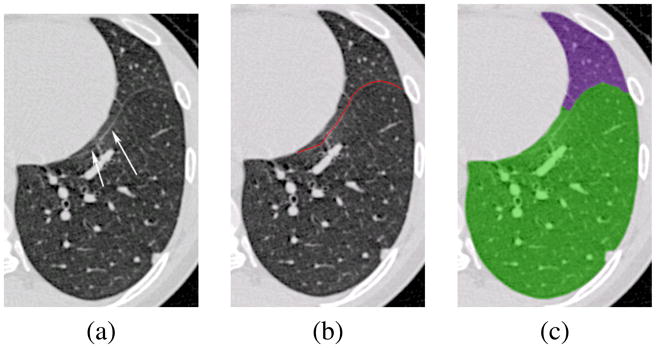
Fig. 10.

(a) Projection images corresponding to cost values, (b) Transverse slice from the same dataset showing incomplete right oblique fissure.

Since the homogeneity of the ridgeness and eigenvector orientations imply that the gradients for both of these values should be low along the fissure and high across the boundary, a front-propagation approach where the speed of propagation is inversely related to these gradients is suited to this segmentation task. Fast marching methods for front-propagation, first proposed by Sethian [22], are appealing because of their robustness to topological changes and their computational efficiency. In the context of incomplete-fissure detection, there are three main aspects to applying the fast marching approach:

1. Seed selection: A set of seeds within the visible fissure region must be selected. The front will propagate outwards from these seeds. To select seeds, we first threshold the cost function projection image and keep only the dark pixels. Next we extract the largest 8-connected region in the thresholded image; the actual, yet incomplete, fissure will be a subset of this region. Finally, we choose pixels near the outer lung border that belong to this thresholded component to form the set of seeds (see Figure 11(a)).

2. Front propagation: The front is propagated from the seed points with a speed that is defined as:

   $$F=min\left(e^{-\alpha |\nabla R_{\sigma }|},e^{-\beta |\nabla A_{\alpha }|}\right),\left(1\right)$$ (1)

   where ∇R_σ and ∇A_σ are the gradients of the ridgeness image and the eigenvector orientation image, respectively. The gradients are computed by convolving with the derivative of a Gaussian with a standard deviation σ. α and β are the weights associated with the two components of the speed term. This formulation ensures that the front slows down at regions where either of the two gradients is large. In our experiments, we used σ = 2 voxels and α = β = 0.0075.

3. The output of the fast-marching algorithm is an image with the propagating front arrival times at each pixel. The segmentation result is generated by thresholding this image, with a suitable value T_thresh, so that only pixels with arrival times less than T_thresh are retained. An empirically determined threshold T_thresh = 2000 time steps was used in all our experiments.

Fig. 11.

Projection images corresponding to incomplete left oblique fissure: (a) Cost values (the red arrow denotes selected seeds), (b) Segmentation result.

The segmentation generated by the above method has some small holes inside it, corresponding to the bright regions inside the homogeneous dark region. A 2-D hole-filling postprocessing step was performed on the segmented image, to generate the segmentation as shown in Figure 11(b). After the detection of the incomplete fissure in the projection image, the segmented result is back-projected onto the optimal fissure surface, as shown in Figure 12(b).

Fig. 12.

(a) Transverse slice showing incomplete fissure, (b) Detected incomplete fissure obtained after analyzing the cost projection image.

C. Algorithm: Fissure extrapolation

After detecting the visible parts of the fissure, our final objective is to complete the incomplete fissure smoothly with an anatomically plausible extrapolation. For a function f in two dimensions, the total squared curvature is given by

$$C\left(z\right)={\int }_S{\left({\nabla }^{2}f\right)}^{2}dS,$$ (2)

where ∇² is the Laplacian operator and S is the surface containing f. For the case of the 2-D function z passing through the data points z_i, i = 1, …, N, it has been shown that a linear combination of the biharmonic Green's functions ϕ(x) = |x|²log(|x| – 1), centered at the data points, gives rise to the minimum curvature biharmonic spline interpolation technique, as shown in [23]. This biharmonic spline interpolation technique gives a smooth extrapolation outside the convex hull of the point set.

The detected incomplete fissure points (e.g., see Figure 12(b)) are used as anchor points needed for the spline interpolation. As illustrated in Figure 4(b), additional anatomical landmarks in the form of airway-tree branchpoints are also used as anchor points. Figure 13 shows the branchpoints EndRMB and EndLMB, which correspond to the end points of the right main bronchi and left main bronchi segments respectively. As can be seen in this figure, the fissures show a general tendency of being directed towards these anatomical landmarks. Using these anchors ensures that the spline interpolation does not generate a surface which is too far off the expected anatomical location. Figure 14 shows an image with an incomplete fissure, and the corresponding watershed segmentation and extrapolated smoothed fissure.

Fig. 13.

(a) Transverse slice from right lung showing the branchpoint EndRMB, (a) Transverse slice from left lung showing the branchpoint EndLMB.

Fig. 14.

Incomplete fissure: (a) Original data set. (b) Watershed segmentation. (c) Extrapolated incomplete fissure.

V. Experimental methods

The lobar segmentation algorithms were assessed in two different experimental conditions: (1) images of normal volunteers taken at different lung volumes and with different reconstruction filters; and (2) clinical images of mild to moderate emphysema subjects. All studies involving humans were gathered under a protocol approved by The University of Iowa institutional review board. All images were acquired on a Siemens Sensation 64 multi-detector CT scanner (MDCT) (Siemens Medical Solutions; Malverne, PA). Reconstructed slice thicknesses ranged from 0.6 to 1.2 mm. The computer used for all of the experiments was a 1.6 GHz AMD Athlon workstation with 2 GB RAM.

A. Images of Normal Volunteers

Data from 12 normal subjects was used to assess lobar fissure segmentation accuracy. The average age was 30 years, and included 5 males and 7 females. For each subject volumetric images covering the thorax were gathered at total lung capacity (TLC) and functional residual capacity (FRC) at approximately 100 mAs. Image reconstructions were performed using a soft (B/B30) and hard (D/B50) reconstruction filter from a single acquisition. Considering all combinations of subjects, lung volume, and filter, 48 data sets were available in all. The automatic lobar segmentation algorithm was applied to each of these data sets.

B. Images of Subjects with Emphysema

Seventeen clinical data sets with mild to moderate emphysema were used to assess the performance of the proposed segmentation method in the presence of lung disease. The average age was 44 years, and included 12 males and 5 females. Each case was read by a radiologist to confirm the presence of emphysema. The fraction of lung voxels below -950 HU was measured to assess the severity of emphysema: nine subjects had less than 5% of the voxels below the cutoff, five subjects had 5 to 10% voxels below -950 HU, and one subject fell in each of the ranges 15-20%, 20-25%, and 30-35% below the threshold. All datasets were acquired at TLC and reconstructed with the B kernel. The lobar segmentation algorithm was applied to each of the 17 data sets.

C. The Gold Standard

To validate performance in the normal and emphysematous data sets, the automatic segmentation results were compared with a manually defined gold-standard. A human image analyst manually traced all the three fissures for each of the 29 cases, marking the fissures as continuous curves on 2-D cross sections. For the right and left oblique fissures, the tracing was done on transverse slices. For the horizontal fissure, the tracing was performed on the sagittal slices because the sagittal view gave the best contrast. Because of the large size the MDCT datasets (typically around 600 slices), the analyst only traced the fissures on every fifth slice.

As we have mentioned before, in a significant fraction of datasets the fissures are incomplete. The fissures are not visible beyond a point, and establishment of a ground-truth is difficult. Therefore, the analyst was instructed only to trace the fissures in regions that they were visible, and to not attempt to extrapolate (or interpolate) regions of missing or incomplete fissures. Since the manual tracing may only be available for the visible portion of the fissure, while the automatic segmentation must span the entire width of the lung, the distance measure used for validation computes the minimum distance of a point on the manual segmentation to a point on the automatic segmentation. This strategy may underestimate the segmentation error if the automatic result deviates far from the manual result.

1) Assessing Segmentation Accuracy

Fissure positioning accuracy was assessed by computing the mean, RMS, and maximum distances between the manually-defined fissures and the computer-defined fissures. For each voxel on the manually-defined contour, the minimum distance to the computer-defined contour was computed as

$$d_i=\underset{j}{min}\left\{\sqrt{{(x_j^A-x_i^M)}^2+{(y_j^A-y_i^M)}^2}\right\},$$

where ( $x_i^M,y_i^M$) is the manually-defined contour voxel location and ( $x_j^A,y_j^A$) is a computer-defined contour voxel location. The mean, RMS and maximum distances to the manually-traced contours were computed using the following equations:

$$\begin{array}{c}{d}_{\text{mean}}=\left(\sum _{i=1}^l{d}_i\right)/l,\\ d_{\text{RMS}}=\sqrt{\sum _{i=1}^l{d}_i^2/l},\\ d_{max}=\underset{i}{max}|d_i|,\end{array}$$

where l is the number of points on the manually-defined contour.

D. Subjects with incomplete fissures

The segmentation results with fissure extrapolation, in the case of incomplete oblique fissures, were visually evaluated by an experienced chest radiologist. The radiologist evaluated 10 segmented data sets using the following numeric scoring system:

• 5 = excellent segmentation and extrapolation of the fissures,

• 4 = one segmentation error; an extrapolated fissure crossed a vessel or passed through a hilar vessel,

• 3 = two segmentation errors; an extrapolated fissure crossed a vessel and passed through a hilar vessel,

• 2 = numerous segmentation errors, usefulness of segmentation in doubt,

• 1 = unusable segmentation.

E. Effects of interpolated image resolution on runtime and segmentation accuracy

As mentioned in Section III-C, runtime depends on the graph size during the fissure refinement step. We performed an experiment to examine the tradeoffs between runtime and accuracy during the optimal surface detection step. For each of the 12 normal TLC/B data sets, we segmented the right oblique fissure three times, corresponding to three different interpolated image resolutions. If we let x_i, y_i and z_i be the original voxel dimensions, the interpolated voxel dimensions in the rotated image are x_o = y_o = z_o = F · min(x_i, y_i, z_i), where F is the resolution scaling factor. We considered F = 1.0 (original resolution), F = 1.2, and F = 1.4. For each of these conditions we calculated the segmentation runtime and the segmentation accuracy compared to the manual analysis.

VI. Results

A. Normal and emphysematous subjects

Table III summarizes the segmentation errors for each of fissures, for each lung volume, and for each reconstruction filter, averaged across all 12 normal data sets. Figure 15 shows the segmentation errors for each of the individual data sets for the case of TLC and filter B for the right oblique fissure. For the clinical images of the subjects with emphysema, Table IV shows the mean (± standard deviation) of the RMS and mean distances averaged over all 17 datasets.

Table III.

Mean of RMS, mean and maximum distance errors, averaged across 12 normal datasets.

Fissure	RMS (mm)	Mean (mm)	Max (mm)
TLC with B kernel
left oblique	2.31 ± 1.72	1.15 ± 0.16	24.06
right oblique	1.57 ± 0.17	1.25 ± 0.16	12.70
right horizontal	1.63 ± 0.99	0.96 ± 0.40	9.46
TLC with D kernel
left oblique	1.81 ± 0.58	1.12 ± 0.30	19.84
right oblique	1.57 ± 0.17	1.26 ± 0.14	11.99
right horizontal	1.43 ± 0.57	0.91 ± 0.22	8.64
FRC with B kernel
left oblique	2.70 ± 1.19	1.50 ± 0.32	23.79
right oblique	2.41 ± 0.58	1.67 ± 0.36	19.90
right horizontal	2.11 ± 1.94	1.23 ± 0.81	11.49
FRC with D kernel
left oblique	1.71 ± 0.60	1.06 ± 0.21	17.28
right oblique	1.88 ± 0.48	1.30 ± 0.29	19.70
right horizontal	2.31 ± 2.18	1.37 ± 1.03	10.05

Fig. 15.

Mean, RMS and maximum distances between manually-defined and computer-defined fissures for the right oblique fissure in normal datasets at TLC reconstructed with the B kernel. The last two columns for (a) show the mean ± standard deviation of the distances calculated over all datasets.

Table IV.

Mean of RMS, mean and maximum distance errors, over 17 datasets with mild to moderate emphysema.

Fissure	RMS (mm)	Mean (mm)	Max (mm)
left oblique	1.86 ± 0.64	1.12 ± 0.30	17.28
right oblique	2.04 ± 0.66	1.17 ± 0.21	19.70
right horizontal	1.50 ± 0.43	0.94 ± 0.23	10.05

One normal data set (subject 7) could not be analyzed at full resolution because the graph search ran out of memory. To resolve this, we set F = 1.2 during the fissure rotation and interpolation step to downsample the data to a more manageable size for this one case. For the 12 normal datasets at TLC reconstructed with the B kernel, three of the twelve cases required one or two seed points to correct the IWT segmentation. For the 17 emphysema cases, four of the cases needed one or two seed points to achieve an acceptable segmentation.

B. Effects of interpolated image resolution on runtime and segmentation accuracy

Table V shows the resulting graph sizes for the fissure ROIs, the runtime for the optimal surface search, and the RMS error between manually-defined and computer-defined fissures for each of the three resolution factors F. The entry marked with an asterisk for subject 7 at resolution factor F = 1.0 are because the graph search ran out of memory during the optimal surface detection at full resolution.

Table V.

Comparison of runtime and accuracy with change in interpolation resolution.

Subject	Resolution factor	Graph size			Time(s)	RMS error (mm)
		X	Y	Z
1	1.0	215	93	406	40.06	1.55
	1.2	179	78	338	16.72	2.23
	1.4	154	66	290	9.08	2.68
2	1.0	222	94	400	27.08	1.88
	1.2	185	79	334	13.23	2.08
	1.4	158	67	286	7.30	2.28
3	1.0	228	104	442	34.55	1.37
	1.2	189	86	369	17.09	1.50
	1.4	162	74	316	9.79	2.00
4	1.0	230	123	391	47.47	1.49
	1.2	192	102	326	21.16	1.67
	1.4	164	88	279	10.90	1.80
5	1.0	229	98	417	32.51	1.70
	1.2	191	82	347	14.81	1.79
	1.4	164	71	298	8.49	1.99
6	1.0	204	104	402	79.67	1.66
	1.2	170	87	335	30.30	1.74
	1.4	146	74	288	14.17	2.10
7	1.0	291	154	532	*	*
	1.2	243	128	444	64.66	1.49
	1.4	208	109	381	29.50	1.52
8	1.0	235	120	380	75.91	1.64
	1.2	197	99	317	31.25	1.81
	1.4	168	85	272	15.48	2.14
9	1.0	230	114	405	34.94	1.21
	1.2	191	95	336	16.11	1.26
	1.4	164	81	289	9.11	1.35
10	1.0	241	114	423	51.28	1.44
	1.2	201	95	351	21.67	1.66
	1.4	172	81	301	11.62	1.82
11	1.0	213	104	431	32.91	1.61
	1.2	177	87	358	14.44	1.76
	1.4	152	75	308	8.23	1.85
12	1.0	261	102	459	60.05	1.75
	1.2	217	86	383	25.89	1.88
	1.4	186	73	328	13.30	2.00

^*The optimal surface detection ran out of memory.

The table shows that the RMS error increases with increasing voxel size. On the other hand, the reduction in the graph-size leads to a very marked reduction in the runtime. A runtime reduction of approximately 75% is observed by using a resolution factor of 1.4.

In Figure 16 we fit a least-squares regression line to the data in Table V, plotted against the graph size. The data for subject 6 and subject 8 at resolution factor 1.0 were excluded from the analysis, as these cases had at least one very incomplete fissure and appeared to be outliers compared to the general pattern observed within the remaining data. The R² value for the regression line was 0.87, which indicates a good fit. The corresponding regression equation (t = 5 * 10⁻⁶D – 7.1237 seconds, where D is the graph size X×Y×Z) can be used to predict the runtime for the fissure segmentation process.

Fig. 16.

Regression line for runtime of graph search versus graph size.

C. Incomplete fissure detection and extrapolation

The incomplete fissure segmentation results were evaluated by an experienced radiologist using the scoring system defined in Section V-D. Out of the 10 data sets evaluated, four data sets were scored as a 5 (“excellent”), four data sets were scored as a 4 (“one error”), and two data sets were scored as a 3 (“two errors”). These results indicate that for these cases the incomplete fissure extrapolation provides a segmentation that is anatomically plausible.

VII. Discussion

The comparison between manually-traced and computer-generated fissures shows a good agreement for the normal data sets, with mean RMS errors less than 2.7 mm across all combinations of fissure, lung volume, and reconstruction kernel. The experiments with emphysematous subjects also show good agreement between the computer-based and manually-traced results, with RMS errors comparable to those for the normal subjects. However, the number of normal and emphysematous test cases used in this study is fairly small, and may not be completely representative of the general population. Further, it should be noted that the majority of the emphysematous subjects had only mild emphysema, with only a few subjects showing more severe emphysema. In subjects with severe emphysema, the presence of large bullae adjacent to the fissures, or very distorted airway and vascular structures, can lead to erroneous results. In the case of diseases which cause increased opacity of the lung parenchyma, like pneumonia, the lung segmentation may be unreliable and the fissure contrast can be reduced, both of which will adversely affect the fissure segmentation result.

Numerically, these results are similar to those obtained using the atlas-based method of Zhang et al. [4], and slightly worse than the semi-automatic approach of Wang et al. [5]. However, our method is faster than the atlas-based approach [4], and has the considerable advantage of being able automatically segment the horizontal fissure, which is not possible with the methods of [4] and [5]. The accuracy of our method, as indicated by the distance errors, should provide reliable quantitative measures such as lobar volumes, lobar tissue histograms, and other lobe-by-lobe measurements.

The gold standard manual segmentations for these experiments were provided by a single trained image analyst. All segmentations were subsequently reviewed by the authors for accuracy and judged acceptable. The differences between the manually-segmented and automatically-segmented fissures should be interpreted in light of the expected intra-observer and inter-observer variabilities for this task; the manual segmentation task is especially difficult and subjective for the horizontal fissures and for the cases with incomplete fissures.

Since the segmentation errors were evaluated by measuring distances from the manual segmentation to the automatic segmentation, the performance may be biased toward the optimistic. Further, since the manual analyst only traced high confidence fissures, more difficult fissure regions might have been excluded from the error calculations, further biasing the results toward the optimistic. The algorithm itself and the associated algorithm parameters were developed and adjusted using a large database of image data from normal volunteers. The 12 normal testing data sets were randomly selected from this same pool, so a small optimistic bias in the results for the normal subjects may also be present because some of the testing data may have been evaluated during the development stage.

While the boundary positioning errors are on the order of 1 to 2 mm RMS, maximum errors on the order of 1 to 2 cm are shown in Table 15 for the right oblique fissure in normal subjects, and these errors are typical for the other fissures and for the emphysematous subjects. Figure 17 shows an explanation of these errors; part of the fissure closely parallels the heart boundary and the optimal surface detection does not follow the fissure all the way to its end point, but instead, jumps to the heart boundary. Since only a small fraction of the fissure surface is parallel to the heart boundary, this segmentation error is not likely to have an appreciable affect on lobar volume calculations. It may be possible to address this problem by changing the parameters C₁, C₂, and C₃ in the cost function C_υ, or by changing the relative weighting between the intensity and ridgeness terms in the C_υ calculation.

Fig. 17.

Case illustrating a large maximum error due to failure to track fissure paralleling heart boundary. (a) Original data set with fissure marked with arrows. (b) Manual tracing. (c) Automatic segmentation.

Occasionally, the initial lobar segmentation step based on the IWT needed manual intervention in the form of additional seed points placed on mislabelled vessels. Usually, this was associated with incomplete fissures where vessel segments cross over from one lobe to another. The re-segmentation with additional markers can be performed in near real-time, which is a major strength of the IWT. From our experiments, 20 to 25% of the cases require some manual seed selection to correct the vessel-guided segmentation. We estimate that the manual interaction to review the initial segmentation results and specify a seed point takes about 30 seconds.

Without specific attention to parallelization, a single-threaded implementation of the process shown in Figure 2 takes 10 to 12 minutes on a 1.6 GHz AMD Athlon workstation. Parallelization can be easily achieved, for instance, in the parallel segmentation of the left and right oblique fissures. For comparison, we estimate that it takes a human analyst about 20 to 30 minutes to trace one oblique fissure on every slice of a CT image, so a complete manual analysis including all three fissures would take approximately 60 to 90 minutes.

VIII. Conclusion

We have presented an automatic method for the segmentation of the lobar fissures on chest CT scans. The method uses the interactive watershed transform, calculated on a vessel distance map, to obtain an initial segmentation. The initial segmentation is refined using 3D optimal surface detection on a ridgeness map. We have tested the method on images from 12 normal and 17 emphysematous subjects and compared the computer results to the results obtained by manual analysis. The resulting lobar segmentations can be used to report image-based measurements, such as mean lung density, on a lobe-by-lobe basis.

Fig. 7.

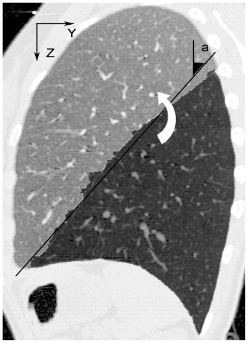
Angle of rotation of the ROI.

References

- 1.Hoffman EA, Ritman EL. Effect of body orientation on regional lung expansion in dog and sloth. J Applied Physiology. 1985;59(2):481–491. doi: 10.1152/jappl.1985.59.2.481. [DOI] [PubMed] [Google Scholar]
- 2.Hubmayr RD, Rodarte JR, Walters BJ, Tonelli FM. Regional ventilation during spontaneous breathing and mechanical ventilation in dogs. J Applied Physiology. 1987;63(6):2467–2475. doi: 10.1152/jappl.1987.63.6.2467. [DOI] [PubMed] [Google Scholar]
- 3.van Rikxoort EM, van Ginneken B, Klik M, Prokop M. Supervised enhancement filters: Application to fissure detection in chest ct scans. IEEE Trans Medical Imaging. 2008;27(1):1–10. doi: 10.1109/tmi.2007.900447. [DOI] [PubMed] [Google Scholar]
- 4.Zhang L, Hoffman EA, Reinhardt JM. Atlas-driven lung lobe segmentation in volumetric X-ray ct images. IEEE Trans Medical Imaging. 2006;25(1):1–16. doi: 10.1109/TMI.2005.859209. [DOI] [PubMed] [Google Scholar]
- 5.Wang J, Betke M, Ko JP. Pulmonary fissure segmentation on ct. Medical Image Analysis. 2006;10(4):530–547. doi: 10.1016/j.media.2006.05.003. [DOI] [PMC free article] [PubMed] [Google Scholar]
- 6.Wiemker R, Bülow T, Blaffert T. Unsupervised extraction of the pulmonary interlobar fissures from high resolution thoracic ct data. Proc of the 19th International Congress and Exhibition - Computer Assisted Radiology and Surgery (CARS); Berlin, Germany. 2005. pp. 1121–1126. [Google Scholar]
- 7.Kuhnigk JM, Hahn HK, Hindennach M, Dicken V, Krass S, Peitgen HO. Lung lobe segmentation by anatomy-guided 3-d watershed transform. Proc SPIE Conf Medical Imaging. 2003;5032:1482–1490. [Google Scholar]
- 8.Zhou X, Hayashi T, Hara T, Fujita H. Proc SPIE Conf Medical Imaging. Vol. 5370. San Diego, ca: 2004. Automatic recognition of lung lobes and fissures from multislice CT images; pp. 1629–1633. [Google Scholar]
- 9.Hayashi K, Aziz A, Ashizawa K, Hayashi H, Nagaoki K, Otsuji H. Radiographic and CT appearances of the major fissures. Radiographics. 2001;21:861–874. doi: 10.1148/radiographics.21.4.g01jl24861. [DOI] [PubMed] [Google Scholar]
- 10.Beichel R, Pock T, Janko C, Zotter RB, Reitinger B, Bornik A, Palágyi K, Sorantin E, Werkgartner G, Bischof H, Sonka M. Liver segment approximation in CT data for surgical resection planning. Proc SPIE Conf Medical Imaging. 2004;5370:1435–1446. [Google Scholar]
- 11.Hu S, Reinhardt JM, Hoffman EA. Automatic lung segmentation for accurate quantitation of volumetric X-ray CT images. IEEE Trans Medical Imaging. 2001;20(6):490–498. doi: 10.1109/42.929615. [DOI] [PubMed] [Google Scholar]
- 12.Tschirren J, Hoffman EA, McLennan G, Sonka M. Intrathoracic airway trees: Segmentation and airway morphology analysis from low-dose CT scans. IEEE Trans Medical Imaging. 2005;24(12):1529–1539. doi: 10.1109/TMI.2005.857654. [DOI] [PMC free article] [PubMed] [Google Scholar]
- 13.Tschirren J, McLennan G, Palágyi K, Hoffman EA, Sonka M. Matching and anatomical labeling of human airway tree. IEEE Trans Medical Imaging. 2005;24(12):1540–1547. doi: 10.1109/TMI.2005.857653. [DOI] [PMC free article] [PubMed] [Google Scholar]
- 14.Shikata H, Hoffman EA, Sonka M. Proc SPIE Conf Medical Imaging. Vol. 5369. San Diego, ca: 2004. Automated segmentation of pulmonary vascular trees from 3-D CT images; pp. 107–116. [Google Scholar]
- 15.Vincent L, Soille P. Watersheds in Digital Spaces: An Efficient Algorithm Based on Immersion Simulations. IEEE Trans Medical Imaging. 1991;13(6):583–598. [Google Scholar]
- 16.Hahn H, Peitgen HO. IWT - interactive watershed transform: A hierarchical method for efficient interactive and automated segmentation of multidimensional grayscale images. Proc SPIE Conf Medical Imaging. 2003;5032:643–653. [Google Scholar]
- 17.Borgefors G. Distance transformation in digital images. Computer Vision, Graphics, and Image Processing. 1986;34(3):344–371. [Google Scholar]
- 18.Wu X, Chen D. Optimal net surface problems with applications. Proc of the 29th International Colloquium on Automata, Languages and Programming (ICALP) 2002 Jul;:1029–1042. [Google Scholar]
- 19.Li K, Wu X, Chen DZ, Sonka M. Optimal Surface Segmentation in Volumetric Images-A Graph-Theoretic Approach. IEEE Trans Patt Anal Machine Intell. 2006;28(1):119–134. doi: 10.1109/TPAMI.2006.19. [DOI] [PMC free article] [PubMed] [Google Scholar]
- 20.Lo´pez AM, Lloret D, Serrat J, Villanueva JJ. Multilocal creaseness based on the level-set extrinsic curvature. Comp Vision and Image Understanding. 2000;77(2):111–144. [Google Scholar]
- 21.Silvela J, Portillo J. Breadth-First search and its application to image processing problems. IEEE Trans Image Proc. 2001;10(8):1194–1199. doi: 10.1109/83.935035. [DOI] [PubMed] [Google Scholar]
- 22.Sethian JA. Fast marching methods. SIAM Review. 1999;41(2):199–235. [Google Scholar]
- 23.Sandwell DT. Biharmonic spline interpolation of GEOS-3 and SEASAT altimeter data. Geophysical Research Letters. 1987;2:139–142. [Google Scholar]