Treating ion distribution with Gaussian-based smooth dielectric function in DelPhi

Abstract

The standard treatment of ions in the framework of the Poisson-Boltzmann equation relies on molecular surfaces, which are commonly constructed along with the Stern layer. The molecular surface determines where ions can be present. In the Gaussian-based smooth dielectric function in DelPhi, smooth boundaries between the solute and solvent take the place of molecular surface. However, this invokes the question of how to model mobile ions in the water phase without a definite solute-solvent boundary. This article reports a natural extension of the Gaussian-based smooth dielectric function approach that treats mobile ions via Boltzmann distribution with an added desolvation penalty. Thus, ion concentration near macromolecules is governed by the local electrostatic potential and the desolvation penalty (from being partially desolvated). The approach is tested against the experimental salt dependence of binding free energy on 7 protein-protein complexes and 12 DNA-protein complexes, resulting in Pearson correlations of 0.95 and 0.88, respectively.

A new approach of modeling ions in the framework of Gaussian-based smooth dielectric function in Poisson-Boltzmann equation (PBE) is reported. Thus, in addition to the Boltzmann term in traditional PBE, ions concentration is altered by a solvation penalty when they translocate from bulk solvent to the space regions with lower dielectric constant. To calculate the solvation penalty, this article adds a Born based solvation energy term into PBE. Calculated salt dependence of the binding free energy results in Pearson correlation of 0.88~0.95 with experiments.

Introduction

Continuum electrostatic approaches are essential tools in modeling electrostatic potential and energies in molecular biology. A particular approach is to apply the Poisson-Boltzmann equation (PBE). It delivers potential distribution throughout the space in the presence of mobile ions. The standard PBE method restricts the space where ions can be present¹.

The PBE of complicated biological macromolecules can be solved numerically through finite difference method^1–6 (FDM), boundary element method^7–12 (BEM), finite element method^13–15 (FEM), etc. These methods have been implemented in several programs, such as Delphi¹⁶, APBS¹⁷, UHBD², MIBPB¹⁸, and in the implicit solvent modules of Amber¹⁹ and CHARMM²⁰.

Standard numerical schemes for solving PBE require that the space is divided into two categories, solute regions and solvent regions. Typically, ions are only allowed to be present in the solvent region, which is outside the ion exclusion layer (Stern layer) surrounding the macromolecule. This requires the construction of a sharp molecular surface to provide a definite boundary between solute and solvent.

Recently we implemented a Gaussian-based smooth dielectric function²¹ in DelPhi. This method treats the solvent and solute in the same framework, and does not require the construction of a molecular surface. This approach comes with a question - how should the mobile ions be treated? Here we introduce a natural extension of our development, which treats mobile ions in the framework of PBE by adding a desolvation penalty term in the Boltzmann factor

Theory and Methods

Adding desolvation penalty in the Boltzmann factor

To keep the mobile ions outside the solute, which is described in PBE as a lower dielectric cavity, we introduce a desolvation energy term in the Boltzmann factor of PBE. Essentially, the probability of a given ion to be present at a location depends not only on the electrostatic potential there, but also on the ability of the ion to maintain its interactions with water (its solvation energy). The desolvation energy is the difference between the solvation energy of the ion in bulk water (ε=80) and the solvation energy of the ion at the considered position (in the framework of the Gaussian-based smooth dielectric constant (termed smooth dielectric SD in this work), each position in the modeling space has its own dielectric constant). Thus we calculate the desolvation penalty via the Born equation,

$$\mathrm{\Delta }{G}_{\mathit{solv}}=-\frac{N_A{z}^2{e}^2}{8\pi {\epsilon }_0{r}_0}\left(\frac{1}{{\epsilon }_r}-\frac{1}{{\epsilon }_w}\right)$$ (1)

, where N_A is the Avogadro constant, z is the valence of the ion, e is the elemental charge, ε₀ is the permittivity of vacuum, r₀ is the effective radius of the ion, ε_r is the dielectric constant at a given location, and ε_w is the dielectric constant of bulk water. For computational efficiency, the effective ion radius is approximated using 2.0Å for both cations and anions.

Thus, introducing the desolvation penalty into PBE results in the following modified PBE:

$$\mathit{\nabla }·\left[\epsilon \left(\mathit{r}\right)\mathit{\nabla }\phi \left(\mathit{r}\right)\right]=-4\pi \left({\rho }_{\mathit{solute}}\left(\mathit{r}\right)+{\displaystyle \sum }_{i=1}^N{q}_i{c}^{\mathit{bulk}}\mathit{exp}\left(\frac{-q_i\phi \left(\mathit{r}\right)-\mathrm{\Delta }{G}_{\mathit{solv}}}{RT}\right)\right)$$ (2)

, where $\epsilon \left(\mathit{r}\right)$, $\phi \left(\mathit{r}\right)$, and ${\rho }_{\mathit{solute}}\left(\mathit{r}\right)$ are the dielectric constant, electrostatic potential, and charge density of solute at given locations, respectively - q_i is the ionic charge, $c^{\mathit{bulk}}$ is the ion concentration in bulk solvent, $\mathrm{\Delta }{G}_{\mathit{solv}}$ is the solvation penalty term for ions, R is the ideal gas constant, and T is the temperature.

The solvation energy term in the Born equation is independent from the sign of the ion charge. When the cations and anions in the solvent have the same absolute charge(s), the non-linear Poisson-Boltzmann (NLPB) equation can be further simplified to

$$\mathit{\nabla }·\left[\epsilon \left(\mathit{r}\right)\mathit{\nabla }\phi \left(\mathit{r}\right)\right]=-4\pi \left({\rho }_{\mathit{solute}}\left(\mathit{r}\right)+{\displaystyle \sum }_{i=1}^{N}2q_i{c}^{\mathit{bulk}}\left[\mathit{exp}\left(\frac{-\mathrm{\Delta }{G}_{\mathit{solv}}}{RT}\right)\right]\left[\mathit{sinh}\left(\frac{-q_i\phi \left(\mathit{r}\right)}{RT}\right)\right]\right)$$ (3)

In dilute salt solution, the corresponding linearized Poisson-Boltzmann (LPB) equation is

$$\mathit{\nabla }·\left[\epsilon \left(\mathit{r}\right)\mathit{\nabla }\phi \left(\mathit{r}\right)\right]=-4\pi \left({\rho }_{\mathit{solute}}\left(\mathit{r}\right)+{\displaystyle \sum }_{i=1}^{N}2q_i{c}^{\mathit{bulk}}\left[\mathit{exp}\left(\frac{-\mathrm{\Delta }{G}_{\mathit{solv}}}{RT}\right)\right]\left(\frac{-q_i\phi \left(\mathit{r}\right)}{RT}\right)\right)$$ (4)

In equation (3) and (4), the ΔG_solv term is different from zero only in the vicinity of a macromolecule, and is zero in bulk water. In practice, it is not calculated if the value is known to be zero. As a result, the addition of the solvation energy term affects the computing performance by less than 5%.

To further illustrate the features of the proposed method, we show an example of a single spherical particle in solvent. In the example, we calculate the Coulombic energy and desolvation penalty of a mobile ion in two cases. In both cases, the particle has +1e charge. The mobile ions have +1e charge in case A, and have +5e charge in case B. Purposely, we assigned the mobile ion the same sign as the charged particle.

Figure 1 shows the corresponding energies as a function of distance. At a large distance the desolvation penalty is zero, and becomes negative (favorable) at shorter distances. Note that the Born solvation energy is proportional to square of the net charge. Thus, if two charged particles with the same charge sign form a complex, the solvation energy of the complex is more favorable than the sum of the solvation energies in isolated particles. This is discussed in an earlier article²². Still, if the ions do not carry large net charges, the repulsive Coulombic interaction is stronger, resulting in total energy always opposing the formation of a pair (Fig. 1A). However, if ions carry biologically non-realistic large charges (+5e in Fig. 1B), then the total energy could be slightly favorable at a particular distance. We have purposely outlined this observation, although it has no implication for molecular biophysics as such highly charged ions are not observed in living organisms, simply to explore the limitations of the proposed approach.

Figure 1.

The electrostatic potential energy and solvation energy of a +1e(A) or +5e(B) charge ion versus the distance from a +1e point charge under smooth dielectric boundary condition. r_vdW is the vdW radius of the point charge.

Calculating the salt dependence of binding free energy

The electrostatic component of binding energy ΔG_el(I) is calculated using the identical equations described in a previous study²²

$$\mathrm{\Delta }{G}_{el}\left(I\right)=G_{el}^{AB}\left(I\right)-G_{el}^A\left(I\right)-G_{el}^B\left(I\right)$$ (5)

, where $G_{el}^{AB}\left(I\right)$, $G_{el}^A\left(I\right)$, $G_{el}^B\left(I\right)$ are the electrostatic component of the complex, monomer A, and monomer B, respectively, at a given ion strength [I]. Thus, the ion effect on the free energy at ion strength [I] (referred as “saltation energy”) is

$$\mathrm{\Delta }\mathrm{\Delta }{G}_{el}\left(I\right)=\mathrm{\Delta }{G}_{el}\left(I\right)-\mathrm{\Delta }{G}_{el}\left(I=0\right)$$ (6)

A linear relationship has been found between ΔG_el(I) and ln(I) for protein-protein complexes and DNA-protein complexes in experimental^23,24 and computational^25,26 studies. The slope $\left[\delta \mathrm{\Delta }\mathrm{\Delta }G(I)/\delta \text{ln}\left(I\right)\right]$ between $\mathrm{\Delta }\mathrm{\Delta }{G}_{el}\left(I\right)$ and $\text{ln}(I)$ is defined as the salt dependence of the binding free energy. For a more detailed interpretation, the reader is referred to earlier articles^22,23.

The calculation is performed using DelPhi¹⁶ with internal dielectric constants of 4, 8, and 16, and an external dielectric constant of 80. It employs a new Gaussian based boundary and ion distribution function. The grid size was determined using 50% filling and 0.5Å per grid. Gaussian variance σ is set to 0.93, surface cut is set to 20. The relaxation parameter used in nonlinear iteration is set to 0.7. When the maximum change in iteration is smaller than 0.0001kT/e, the iteration is considered to be converged. Salt concentrations are from 0.00 to 0.50mol/L with a 0.05mol/L interval.

Preparing complex structures

Table 1. Data for the atomic resolution structures determined by NMR or X-ray crystallography, experimental pH reported by the authors, and the pH of calculations. Calculated (via the non-linear PBE) and experimental salt dependences are reported as the slope of the change of the salt component of the binding free energy $\mathrm{\Delta }\mathrm{\Delta }{G}_{el}\left(I\right)$ as a function of the logarithm of the salt concentration $\text{ln}\left(I\right)$, $\left[\delta \mathrm{\Delta }\mathrm{\Delta }G(I)/\delta \text{ln}\left(I\right)\right]$.

Table 1.

Experimental and calculated salt dependence

Complex	PDB code	Chains	Model	Exp pH	Ref	Exp	Calc pH	Calc
Protein-Protein
E9Dnase-Im9	1EMV27	A-B	XRD	7	28	2.17	7	2.18
Barnase-Barstar	1BRS29	A-D	XRD	8	30	0.96	8	1.86
Thrombin-Hirudin	4HTC31	H-I	XRD	7a	24	0.82	7	0.69
Tem_1-Blip	1JTG32	A-B	XRD	7	33	0.40	7	0.06
Amy2-Basi	1AVA34	A-C	XRD	6.5	35	0.35	7	0.29
Hemoglobin tetramer	1A3N36	AB-CD	XRD	7.4	37	0.16	7	−0.16
Lactoglobulin dimer	1BEB38	A-B	XRD	3	39	−1.62	3	−1.71
DNA-Protein
desANTP	9ANT40	CD-A	XRD	6	41	6.9	6	11.26
desNK2	1NK342	AB-P	NMR-1	6	41	5.5	6	11.19
MAT-α2	1APL43	AB-C	XRD	6	41	5.8	6	9.88
Engrailed	3HDD44	CD-A	XRD	6	41	6.6	6	10.67
LEF79	2LEF45	BC-A	NMR-1	6	46	6.8	6	14.73
SRY	1J4647	BC-A	NMR-1	6	46	8.5	6	15.46
D74	1QRV48	CD-A	XRD	6	46	2.5	6	5.24
NHP6A	1J5N49	BC-A	NMR-1	6	46	4.1	6	11.80
IRF-DBD1	1IF150	CD-A	XRD	7.4	51	1.4	7	6.27
IRF-DBD3	1T2K52	EF-A	XRD	7.4	51	3.3	7	6.34
CoreDBD2	2EZD53	BC-A	NMR-1	7	54	2.1	7	8.07
DBD3	2EZF53	BC-A	XRD	7	54	2.6	7	5.97

^aThe experimental pH is not available in literature.

To test the performance of this approach, we applied it to model the salt dependence of binding free energy on 7 protein-protein (P-P) and 12 DNA-protein (D-P) complexes, for which we were able to obtain experimental data (see Method section). All available protein-protein and DNA-protein complexes were obtained from the Protein Data Bank (PDB)⁵⁵. Table 1 shows the details about the structures and experimental conditions. The protonation state of residues was assigned using the DelPhiPKa⁵⁶ web server, using CHARMM 27 force field. The individual protein(s)/DNA and the complex underwent 1000 steps of conjugated gradient energy minimization with 1kcal/(mol·Å) harmonic restraint on backbone atoms using CHARMM software and CHARMM 27 force field. The Generalized Born⁵⁷ solvation energy was used during the minimization. All neutral histidine residues are assumed as HSD conformation.

Evaluating the grid dependence of the salt component in binding free energy

To evaluate the grid dependence of the salt component in binding free energy $(\mathrm{\Delta }\mathrm{\Delta }{G}_{el}(I))$, a system containing an arginine and a glutamate acid amino acids (Arg-Glu) was employed. The residues were taken from a salt bridge in Barnase-Barstar complex, and underwent 2000 steps energy minimization in CHARMM. The saltation energy component $\mathrm{\Delta }\mathrm{\Delta }{G}_{el}(I)$ was calculated by eq.(6) at salt concentration I equal to 0.15mol/L.

The electrostatic energies were calculated using DelPhi smooth dielectric boundary condition. The dielectric constant was set to 4 for solute and 80 for solvent. Gaussian variance σ was set to 0.93, relaxation parameter was set to 0.7, and the convergence criteria was set to 0.0001kT/e.

Results

Comparison with experiments

Following previous works, we compared the slope of the change in binding free energy ΔG_el(I) as a function of the logarithm of the salt concentration $\text{ln}\left(I\right)$, $\left[\delta \mathrm{\Delta }\mathrm{\Delta }G(I)/\delta \text{ln}\left(I\right)\right]$. For a more detailed interpretation, readers may refer to earlier articles^22,23.

The calculated salt dependence of the binding free energies shows 0.88 or higher Pearson correlation with experimental results (Fig. 2), for both P-P complexes and D-P complexes. The fitting slope (k) from Non-Linear Poisson Boltzmann (NLPB, Fig. 2B) is closer to 1 than the slope from Linearized Poisson Boltzmann (LPB, Fig. 2A), for both P-P and D-P complexes. The calculated salt dependence is not affected by varying the dielectric constant of the solute (Fig. 2CD).

Figure 2.

Comparison of experimental and calculated salt dependence of binding free energies. Calculated values are from linearized PBE (A) and non-linear PBE (BCD) under solute dielectric constant 4 (AB), 8 (C), and 16 (D). R is the correlation coefficient, k is the slope of the fitting curve. The word “Gaussian” is used to indicate that “Gaussian-based smooth dielectric function” was used in PBE.

For protein-protein complexes, the calculated salt dependence from LPB (Fig.2A) and NLPB (Fig. 2B) are consistent with experimental data on the magnitude. The slope (k) of NLPB is 1.09, 23% smaller than the 1.41 from LPB. As the P-P complexes studied here carry low net charges, the calculated salt dependence ( $\delta \mathrm{\Delta }\mathrm{\Delta }G(I)/\delta \text{ln}[I]$) from LPB is generally close to those from NLPB. Similar results have been found in a previous study²². A notable exception is the E9Dnase-Im9 complex, which is highest in charge among all P-P complexes. In this case, the LPB results in a salt dependence of 1.31, while the experimental data is 2.17. NLPB gives a calculated salt dependence of 2.18, which is extremely close to the experimental value.

Compared with our earlier results using the standard two-dielectric model, we observe that the calculated salt dependences here are slightly magnified, because the present method allows salt ions to exist at regions closer to the solute (as compared with sharp-boundary two-dielectric approach). Furthermore, it assigns lower dielectric values at the boundary, and results in stronger electrostatic interactions.

For DNA-protein complexes, although both LPB (Fig. 2A) and NLPB (Fig. 2B) show similar correlation to experimental data, the slope from NLPB is 1.30 (40% smaller than the 2.15 from LPB). Earlier studies have shown that NLPB performs better on highly charged systems, including DNA complexes. Our results show the same trend. Although the calculated DNA-protein salt effects from LPB show good correlation with experimental data, the values are more exaggerated than those from NLPB.

The calculated salt dependences for DNA-protein complexes from NLPB are still 1.5–2 times as large as the experimental values - not because of the slope, but because of the interception. For P-P complexes, the results are 20% greater than the experimental values. According to the counterion condensation theory⁵⁸, the salt dependence is related to the amount of charges on the contact surface. The higher the charges are, the larger the salt dependence is. Some of these charges are likely to bind to oppositely charged ions in solvent, and the ions therefore become localized. These ions partially neutralize the charges on the binding surface. However, these localized ions are not counted in PBE. This may be one of the reasons for the exaggerated salt dependence. Usually, DNAs are highly negatively charged, and proteins that bind to DNA carry high positive charges on the binding domains. Thus, the salt dependence of D-P complexes is more exaggerated than in P-P complexes. The problem may be resolved by including the explicit ions in complexes^59–62.

Dependence on grid parameters

To study the sensitivity of the results to the grid parameters, we model the saltation component in binding free energy of an artificial system made by Arg-Glu pair at physiological conditions. The saltation energy is given by the difference in electrostatic component of binding free energy ( $\mathrm{\Delta }\mathrm{\Delta }{G}_{el}(I)$) in eq.(6)) under salt concentration [I] equals to 0.15mol/L and 0, respectively.

The precision of grid based PBE solvers depends on the grid resolution. The results converge gradually as grid resolution increases (Fig. 3). If we use the results from 10 grids/Å and 20% filling as a reference value, results from grid resolution higher than 4 differ from the reference by less than 0.03kT. Results from lower grid resolution varies more but still the variation is very small.

Figure 3.

Saltation energy ( $\mathrm{\Delta }\mathrm{\Delta }{G}_{el}(I)$) in the binding of Arg-Glu complex under grid resolution 0.5 to 10 grids/Å. Tested using box filling 20%, 50% and 80%.

The sensitivity of the results also depends on the size of the simulation box. The largest dimension of the Arg-Glu complex is ~11Å. Grid fillings of 20%, 50%, and 80% correspond to box sizes of 55Å, 22Å, and 14Å, respectively. Results show marginal dependence on the size of the box. When large box size is used, the method gives small variance to reference value, even at lower grid resolutions. The reason for that is that in the SD method, as the distance to atom center increases, the dielectric constant of the boundary grid points changes from ε_s to ε_w. When the distance is larger than $3\sigma R_{\mathit{vdw}}$, the ε_r approaches ε_w. Thus, to obtain results less sensitive to the grid resolution (Fig. 3), the filling of the box should not be large to allow the ε_r reach ε_w value.

Furthermore, the SD method shows less than 0.15 kT variance in both translocational (Fig. 4A) and rotational (Fig. 4B) tests of salt component of binding free energy. Similar performance has been observed in an earlier study²¹.

Figure 4.

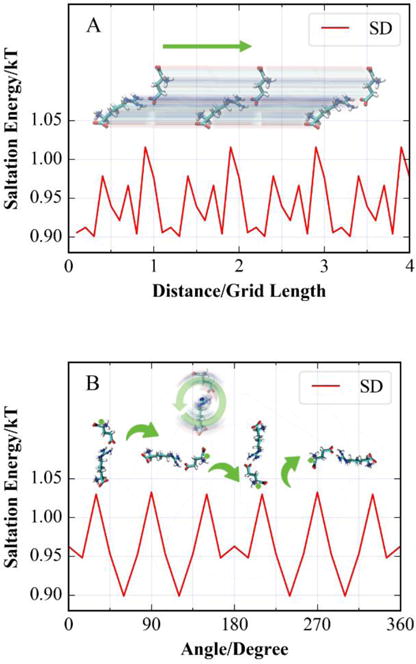
$\mathrm{\Delta }\mathrm{\Delta }{G}_{el}$ of the Arg-Glu complex when the complex is under translocational (A) or rotational (B) offset on the cubic grid. The box is 50% filled and resolution is 2 grids per Å. The grids in figures do not represent actual grids in calculation.

In this article, the SD method is tested in DelPhi using uniform grid resolution. Multigrid³ methods show better precision than the uniform grid method and it is possible that the presented approach may be improved if complemented with multigrid method.

Computational time

The SD method has more boundary grid points than the standard discrete dielectric boundary condition approach, and costs more computing time. In the DelPhi PBE solver, the non-boundary points have the same dielectric constant as all the surrounding grid points, and are treated using the Laplacian equation. The boundary points have different dielectric constants than their surrounding grid points, and are treated using the standard PBE. Based on Nicholls’ estimation¹, calculating regular PBE requires ~4 times more flops than calculating with Laplacian. In the standard two-dielectric method approach, less than 10% grid points are boundary grid points. This percentage increases to 30% or higher in the SD method, depending on the size and shape of the solute. As a result, the SD method usually costs 1.5–2 more computing time as compared to the two-dielectric method on the same grid size.

Conclusions

In conclusion, we demonstrate a new approach that treats ions in conjunction with their desolvation penalty in the framework of the Gaussian-based smooth dielectric function in PBE. It has been tested and compared with experimental data, and was shown to be very successful in modeling the salt dependence of protein-protein and DNA-protein binding free energy. Pearson correlations of 0.88 and 0.95 have been achieved when compared with experimental data. Compared to the standard treatment of ions, the presented approach better reflects physical reality. Indeed, biological macromolecules are, in fact, not rigid objects. Drawing a sharp boundary between solute and solvent does not reflect dynamical nature of the solute-water phase. Instead, the modeling should involve a transition region with mixed properties, and to allow ions to partially penetrate within it.

It should be pointed out that the treatment of ions in bulk water phase (away from the macromolecule) in the present model is identical to the treatment of ions in traditional PB approach. However, close to macromolecular surface, so termed macromolecule-water transition zone, the Boltzmann factor weight is altered by the desolvation penalty that particular type of ions would experience if present at the grid point of interest. If one replaces the smooth Gaussian-based dielectric function with the traditional two-dielectric sharp border, then the present model provides the same ion treatment as the traditional PB approach, which Stern layer equal to the radius of type of ions.

The presented approach has already been implemented in DelPhi, which can be downloaded from http://compbio.clemson.edu/delphi.

References and Notes

- 1.Nicholls A, Honig B. Journal of Computational Chemistry. 1991;12(4):435–445. [Google Scholar]
- 2.Davis ME, Mccammon JA. Journal of Computational Chemistry. 1989;10(3):386–391. [Google Scholar]
- 3.Holst M, Saied F. Journal of Computational Chemistry. 1993;14(1):105–113. [Google Scholar]
- 4.Luo R, David L, Gilson M. K. Journal of Computational Chemistry. 2002;23(13):1244–1253. doi: 10.1002/jcc.10120. [DOI] [PubMed] [Google Scholar]
- 5.Luty BA, Davis ME, Mccammon JA. Journal of Computational Chemistry. 1992;13(6):768–771. [Google Scholar]
- 6.Rocchia W, Alexov E, Honig B. Journal of Physical Chemistry B. 2001;105(28):6507–6514. [Google Scholar]
- 7.Boschitsch AH, Fenley MO, Zhou HX. Journal of Physical Chemistry B. 2002;106(10):2741–2754. [Google Scholar]
- 8.Hoshi H, Sakurai M, Inoue Y, Chujo R. Journal of Chemical Physics. 1987;87(2):1107–1115. [Google Scholar]
- 9.Lu BZ, Cheng XL, Huang JF, McCammon J. P Natl Acad Sci USA. 2006;103(51):19314–19319. doi: 10.1073/pnas.0605166103. [DOI] [PMC free article] [PubMed] [Google Scholar]
- 10.Rashin AA. J Phys Chem-Us. 1990;94(5):1725–1733. [Google Scholar]
- 11.Yoon BJ, Lenhoff AA. Journal of Computational Chemistry. 1990;11(9):1080–1086. [Google Scholar]
- 12.Zauhar RJ, Morgan R. Journal of Computational Chemistry. 1988;9(2):171–187. [Google Scholar]
- 13.Baker N, Holst M, Wang F. Journal of Computational Chemistry. 2000;21(15):1343–1352. [Google Scholar]
- 14.Cortis CM, Friesner RA. Journal of Computational Chemistry. 1997;18(13):1570–1590. [Google Scholar]
- 15.Holst M, Baker N, Wang F. Journal of Computational Chemistry. 2000;21(15):1319–1342. [Google Scholar]
- 16.Li L, Li CA, Sarkar S, Zhang J, Witham S, Zhang Z, Wang L, Smith N, Petukh M, Alexov E. Bmc Biophys. 2012;5 doi: 10.1186/2046-1682-5-9. [DOI] [PMC free article] [PubMed] [Google Scholar]
- 17.Baker NA, Sept D, Joseph S, Holst MJ, McCammon JA. P Natl Acad Sci USA. 2001;98(18):10037–10041. doi: 10.1073/pnas.181342398. [DOI] [PMC free article] [PubMed] [Google Scholar]
- 18.Chen DA, Chen Z, Chen CJ, Geng WH, Wei G. Journal of Computational Chemistry. 2011;32(4):756–770. doi: 10.1002/jcc.21646. [DOI] [PMC free article] [PubMed] [Google Scholar]
- 19.Holst MJ, Saied F. Journal of Computational Chemistry. 1995;16(3):337–364. [Google Scholar]
- 20.Im W, Beglov D, Roux B. Comput Phys Commun. 1998;111(1–3):59–75. [Google Scholar]
- 21.Li L, Li C, Zhang Z, Alexov E. Journal of chemical theory and computation. 2013;9(4):2126–2136. doi: 10.1021/ct400065j. [DOI] [PMC free article] [PubMed] [Google Scholar]
- 22.Bertonati C, Honig B, Alexov E. Biophysical Journal. 2007;92(6):1891–1899. doi: 10.1529/biophysj.106.092122. [DOI] [PMC free article] [PubMed] [Google Scholar]
- 23.Privalov PL, Dragan AI, Crane-Robinson C. Nucleic Acids Research. 2011;39(7):2483–2491. doi: 10.1093/nar/gkq984. [DOI] [PMC free article] [PubMed] [Google Scholar]
- 24.Stone SR, Dennis S, Hofsteenge J. Biochemistry. 1989;28(17):6857–6863. doi: 10.1021/bi00443a012. [DOI] [PubMed] [Google Scholar]
- 25.Thomas AS, Elcock AH. Journal of the American Chemical Society. 2006;128(24):7796–7806. doi: 10.1021/ja058637b. [DOI] [PubMed] [Google Scholar]
- 26.Russo C. Florida State University. 2010 [Google Scholar]
- 27.Kuhlmann UC, Pommer AJ, Moore GR, James R, Kleanthous C. Journal of Molecular Biology. 2000;301(5):1163–1178. doi: 10.1006/jmbi.2000.3945. [DOI] [PubMed] [Google Scholar]
- 28.Wallis R, Moore GR, James R, Kleanthous C. Biochemistry. 1995;34(42):13743–13750. doi: 10.1021/bi00042a004. [DOI] [PubMed] [Google Scholar]
- 29.Buckle AM, Schreiber G, Fersht AR. Biochemistry. 1994;33(30):8878–8889. doi: 10.1021/bi00196a004. [DOI] [PubMed] [Google Scholar]
- 30.Schreiber G, Fersht AR. Biochemistry. 1993;32(19):5145–5150. doi: 10.1021/bi00070a025. [DOI] [PubMed] [Google Scholar]
- 31.Rydel TJ, Tulinsky A, Bode W, Huber R. Journal of Molecular Biology. 1991;221(2):583–601. doi: 10.1016/0022-2836(91)80074-5. [DOI] [PubMed] [Google Scholar]
- 32.Lim D, Park HU, De Castro L, Kang SG, Lee HS, Jensen S, Lee KJ, Strynadka NCJ. Nature structural biology. 2001;8(10):848–852. doi: 10.1038/nsb1001-848. [DOI] [PubMed] [Google Scholar]
- 33.Albeck S, Schreiber G. Biochemistry. 1999;38(1):11–21. doi: 10.1021/bi981772z. [DOI] [PubMed] [Google Scholar]
- 34.Vallee F, Kadziola A, Bourne Y, Juy M, Rodenburg KW, Svensson B, Haser R. Struct Fold Des. 1998;6(5):649–659. doi: 10.1016/s0969-2126(98)00066-5. [DOI] [PubMed] [Google Scholar]
- 35.Nielsen PK, Bonsager BC, Berland CR, Sigurskjold BW, Svensson B. Biochemistry. 2003;42(6):1478–1487. doi: 10.1021/bi020508+. [DOI] [PubMed] [Google Scholar]
- 36.Tame JRH, Vallone B. Acta Crystallogr D. 2000;56:805–811. doi: 10.1107/s0907444900006387. [DOI] [PubMed] [Google Scholar]
- 37.Doyle ML, Holt JM, Ackers GK. Biophysical chemistry. 1997;64(1–3):271–287. doi: 10.1016/s0301-4622(96)02235-1. [DOI] [PubMed] [Google Scholar]
- 38.Brownlow S, Cabral JHM, Cooper R, Flower DR, Yewdall SJ, Polikarpov I, North ACT, Sawyer L. Structure. 1997;5(4):481–495. doi: 10.1016/s0969-2126(97)00205-0. [DOI] [PubMed] [Google Scholar]
- 39.Sakurai K, Oobatake M, Goto Y. Protein Science. 2001;10(11):2325–2335. doi: 10.1110/ps.17001. [DOI] [PMC free article] [PubMed] [Google Scholar]
- 40.Fraenkel E, Pabo C. O. Nature structural biology. 1998;5(8):692–697. doi: 10.1038/1382. [DOI] [PubMed] [Google Scholar]
- 41.Dragan AI, Li ZL, Makeyeva EN, Milgotina EI, Liu YY, Crane-Robinson C, Privalov PL. Biochemistry. 2006;45(1):141–151. doi: 10.1021/bi051705m. [DOI] [PubMed] [Google Scholar]
- 42.Gruschus JM, Tsao DH, Wang LH, Nirenberg M, Ferretti JA. Biochemistry. 1997;36(18):5372–5380. doi: 10.1021/bi9620060. [DOI] [PubMed] [Google Scholar]
- 43.Wolberger C, Vershon AK, Liu BS, Johnson AD, Pabo CO. Cell. 1991;67(3):517–528. doi: 10.1016/0092-8674(91)90526-5. [DOI] [PubMed] [Google Scholar]
- 44.Fraenkel E, Rould MA, Chambers KA, Pabo CO. Journal of Molecular Biology. 1998;284(2):351–361. doi: 10.1006/jmbi.1998.2147. [DOI] [PubMed] [Google Scholar]
- 45.Love JJ, Li XA, Case DA, Giese K, Grosschedl R, Wright PE. Nature. 1995;376(6543):791–795. doi: 10.1038/376791a0. [DOI] [PubMed] [Google Scholar]
- 46.Dragan AI, Read CM, Makeyeva EN, Milgotina EI, Churchill MEA, Crane-Robinson C, Privalov PL. Journal of Molecular Biology. 2004;343(2):371–393. doi: 10.1016/j.jmb.2004.08.035. [DOI] [PubMed] [Google Scholar]
- 47.Stawiski EW, Gregoret LM, Mandel-Gutfreund Y. Journal of Molecular Biology. 2003;326(4):1065–1079. doi: 10.1016/s0022-2836(03)00031-7. [DOI] [PubMed] [Google Scholar]
- 48.Murphy FV, Sweet RM, Churchill MEA. Embo Journal. 1999;18(23):6610–6618. doi: 10.1093/emboj/18.23.6610. [DOI] [PMC free article] [PubMed] [Google Scholar]
- 49.Masse JE, Wong B, Yen YM, Allain FHT, Johnson RC, Feigon J. Journal of Molecular Biology. 2002;323(2):263–284. doi: 10.1016/s0022-2836(02)00938-5. [DOI] [PubMed] [Google Scholar]
- 50.Escalante CR, Yie JM, Thanos D, Aggarwal AK. Nature. 1998;391(6662):103–106. doi: 10.1038/34224. [DOI] [PubMed] [Google Scholar]
- 51.Hargreaves VV, Makeyeva EN, Dragan AI, Privalov PL. Biochemistry. 2005;44(43):14202–14209. doi: 10.1021/bi051115o. [DOI] [PubMed] [Google Scholar]
- 52.Panne D, Maniatis T, Harrison SC. Embo Journal. 2004;23(22):4384–4393. doi: 10.1038/sj.emboj.7600453. [DOI] [PMC free article] [PubMed] [Google Scholar]
- 53.Huth JR, Bewley CA, Jackson BM, Hinnebusch AG, Clore GM, Gronenborn AM. Protein Science. 1997;6(11):2359–2364. doi: 10.1002/pro.5560061109. [DOI] [PMC free article] [PubMed] [Google Scholar]
- 54.Dragan AI, Liggins JR, Crane-Robinson C, Privalov PL. Journal of Molecular Biology. 2003;327(2):393–411. doi: 10.1016/s0022-2836(03)00050-0. [DOI] [PubMed] [Google Scholar]
- 55.Berman HM, Westbrook J, Feng Z, Gilliland G, Bhat TN, Weissig H, Shindyalov IN, Bourne PE. Nucleic Acids Research. 2000;28(1):235–242. doi: 10.1093/nar/28.1.235. [DOI] [PMC free article] [PubMed] [Google Scholar]
- 56.Wang L, Zhang M, Alexov E. Bioinformatics. 2016;32(4):614–615. doi: 10.1093/bioinformatics/btv607. [DOI] [PMC free article] [PubMed] [Google Scholar]
- 57.Im WP, Lee MS, Brooks CL. Journal of Computational Chemistry. 2003;24(14):1691–1702. doi: 10.1002/jcc.10321. [DOI] [PubMed] [Google Scholar]
- 58.Manning GS. Journal of Chemical Physics. 1969;51(3):924. -&. [Google Scholar]
- 59.Auffinger P, Westhof E. Journal of Molecular Biology. 2000;300(5):1113–1131. doi: 10.1006/jmbi.2000.3894. [DOI] [PubMed] [Google Scholar]
- 60.Varnai P, Zakrzewska K. Nucleic Acids Research. 2004;32(14):4269–4280. doi: 10.1093/nar/gkh765. [DOI] [PMC free article] [PubMed] [Google Scholar]
- 61.Petukh M, Zhenirovskyy M, Li C, Li L, Wang L, Alexov E. Biophysical Journal. 2012;102(12):2885–2893. doi: 10.1016/j.bpj.2012.05.013. [DOI] [PMC free article] [PubMed] [Google Scholar]
- 62.Ye X, Cai Q, Yang W, Luo R. Biophysical Journal. 2009;97(2):554–562. doi: 10.1016/j.bpj.2009.05.012. [DOI] [PMC free article] [PubMed] [Google Scholar]