Use of Sub-ensembles and Multi-template Observers to Evaluate Detection Task Performance for Data That are Not Multivariate Normal

Abstract

The Hotelling Observer (HO) is widely used to evaluate image quality in medical imaging. However, applying it to data that are not multivariate-normally (MVN) distributed is not optimal. In this paper, we apply two multi-template linear observer strategies to handle such data. First, the entire data ensemble is divided into sub-ensembles that are exactly or approximately MVN and homoscedastic. Next, a different linear observer template is estimated for and applied to each sub-ensemble. The first multi-template strategy, adapted from previous work, applies the HO to each sub-ensemble, calculates the area under the receiver operating characteristics curve (AUC) for each sub-ensemble, and averages the AUCs from all the sub-ensembles. The second strategy applies the Linear Discriminant (LD) to estimate test statistics for each sub-ensemble and calculates a single global AUC using the pooled test statistics from all the sub-ensembles. We show that this second strategy produces the maximum AUC when only shifting of the HO test statistics is allowed. We compared these strategies to the use of a single HO template for the entire data ensemble by applying them to the non-MVN data obtained from reconstructed images of a realistic simulated population of myocardial perfusion SPECT studies with the goal of optimizing the reconstruction parameters. Of the strategies investigated, the multi-template LD strategy yielded the highest AUC for any given set of reconstruction parameters. The optimal reconstruction parameters obtained by the two multi-template strategies were comparable and produced higher AUCs for each sub-ensemble than the single-template HO strategy.

I. Introduction

IN medical imaging, image quality is objectively assessed in terms of the performance of an observer on a relevant task [1]. Relevant tasks include classification and estimation tasks. For binary classification (i.e., detection) tasks with known signal locations, performance can be characterized by the receiver operating characteristics (ROC) curve. The area under the ROC curve (AUC) is an often-used figure of merit for detection tasks.

Several model observers have been formulated for objectively evaluating image quality on detection tasks. The ideal observer (IO) uses all the statistical information about the data and yields the maximum AUC of all possible observers [2, 3]. However, the IO is often complicated and difficult to compute, and may not predict human observer performance. Therefore, linear observers, in particular, the Hotelling observer (HO), have been widely used [4]. The HO uses the first- and second-order statistics of the image data to compute an observer template. When the data follow a multivariate normal (MVN) distribution with equal covariances under the signal-absent and signal-present hypotheses, the HO has equivalent performance to the IO.

The channelized version of the HO, referred to as the CHO, is also a commonly used model observer. When used with appropriate anthropomorphic channels that model the human visual system, the CHO has been shown to agree well with human performance for signal known exactly (SKE)/background known exactly (BKE) tasks [5, 6] and SKE-lumpy backgrounds tasks [7]. For SKE tasks where the channel outputs, often referred to as feature vectors, are MVN distributed and homoscedastic (i.e., when the two classes have equal covariance matrices), the CHO is theoretically optimal [8]. The CHO has been widely used to predict human performance for SKE tasks [6, 9, 10].

Clinical tasks have variability in both signal and background. The signal and the background may be known only statistically, thus resulting in a signal known statistically (SKS) and background known statistically (BKS) task. In the context of nuclear medicine imaging, signals vary in tracer uptake, size, and position. Similarly, variations in normal organ and tissue size, shape and uptake result in background variability. In recent work, we have shown that signal or background variations, alone or in combination, can result in very non-MVN and even multi-modal [11] distributions of channel outputs.

It is thus desirable to have observer strategies that can handle non-MVN data. The IO can, in principle, optimally treat non-MVN data. Expressions for IO performance typically require explicit knowledge of the probability distribution of the data. However, for realistic data, these are often not known. Methods have been proposed for calculating IO performance in cases of background variability with realistic data [12–15]. In principle, these could be applied to channel output data for cases with statistical signal and background variations. However, these methods are very computationally intensive.

We observed that non-MVN data (e.g., feature vectors) resulting from the statistical variations mentioned above were often multi-modal, and suitable partitioning of the data could produce sub-ensembles with near-Gaussian distributions. The data could thus be treated as a Gaussian mixture model. The parameters of the model could be estimated from the data, and the IO performance could then be calculated from these. However, estimating the Gaussian-mixture-model parameters would be complicated, and this method has not, to our knowledge, been investigated in the context of image quality evaluation. As an alternative, several strategies based on linear observers have been proposed.

The HO has frequently been applied to data (feature vectors) with signal and background variability [16–19]. Since one HO template is applied to all the images in the ensemble, we refer to this as a single-template HO strategy. However, for non-MVN distributed data, the application of the HO to these tasks can be problematic [20].

As noted, the non-MVN nature of the data was observed to arise from signal and background variations. Previous authors have proposed and applied a multi-template observer strategy to the data in SKS task [21–25]. In this strategy, a template (i.e., an instance of the linear observer whose dot product with an input data item yields the test statistic for that item) is generated for each possible realization of the signal. The test statistics for each image are obtained by applying all templates to the image data (projection data or feature vector) and are then combined using the optimal sum of likelihood rule [26]. Note that this observer strategy is not equivalent to the IO, and it is applicable only to the case where there are a finite number of signal types. In these studies, empirical evidence was provided for task performance correlations between human observers and this model observer strategy for the SKS task. This strategy is computationally expensive compared to a single-template observer strategy, especially when the number of possible signal types is very large.

Eckstein et al. [21, 27] have demonstrated that human performance on an SKS task can be approximated by the performance of a simplified signal known exactly but variable (SKEV) task for the range of signal type variations in their study. An SKEV task is one in which the signals vary from image to image but the observers know the exact signal type present in the image. They also proposed a multi-template strategy for SKEV tasks. Again, this strategy can still be computationally expensive when the number of possible signal types is very large.

In this work, we describe two multi-template strategies to evaluate detection task performance when the data are non-MVN distributed. It should be noted that the focus is not on providing a general solution to SKS or SKEV tasks, but on handling the problem of non-MVN data, which can arise due to signal or background variability. The strategies we provide are based on a sub-ensemble-based approach: the non-MVN data are divided into sub-ensembles with MVN-distributed and homoscedastic data. A different observer template is estimated and applied for each such sub-ensemble. We present two strategies for using the data in the sub-ensembles. In the first strategy, we adapt a multi-template HO strategy initially proposed by Eckstein et al. for SKEV tasks [21, 27]. We also propose a novel multi-template linear discriminant strategy and discuss the theoretical motivation and the optimality of the classification performance in terms of the AUC for this strategy. We compared these two strategies with the commonly used and computationally-inexpensive single-template HO strategy. We applied these strategies to optimize the reconstruction parameters for a defect detection task performed on a realistic dual isotope myocardial perfusion SPECT (MPS) simulated dataset [28]. The channel outputs from the images in the study are non-MVN. The three strategies were compared in terms of their AUCs and the ranges of optimal parameters.

II. Theory

In this section, we describe the theory of the two multi-template linear observer strategies to handle non-MVN distributed data using a sub-ensemble-based approach proposed in this paper. These are the major contribution of this work. As a prelude to presenting this theory, we first discuss the sub-ensemble-based approach in general and methods used to partition the data into sub-ensembles.

A. Sub-ensemble-based Approach

The proposed method for handling non-MVN distributed data is to divide the data into sub-ensembles that are exactly or approximately MVN distributed and homoscedastic. We can then apply optimal linear observers to each sub-ensemble and use the test statistics to compute a figure of merit, as described in Sections II.B and II.C.

There may not be a unique sub-ensemble partitioning method that provides subsets of data that meet the MVN and homoscedasticity conditions. The problem of partitioning the data in the general case is potentially very complicated. Thus, in this paper, we do not provide either a general or an optimal method. Instead, we provide two feasible partitioning methods that were applicable to the data used in this work. The first is based on partitioning the data into SKE tasks; the second is to use characteristics used in generating the data such as the defect type (i.e., location, extent, and severity) and phantom anatomical parameters. This latter approach is, for reasons described below, the one used in the remainder of the paper. In the discussion section, we discuss the possibility of using data-centric approaches, such as clustering methods, to provide a more general solution to this partitioning problem.

The MVN and homoscedasticity conditions are often, though not always, satisfied when each sub-ensemble represents an SKE task. Thus, one straight-forward method is to partition the data into different sub-ensembles for each different SKE task. However, this SKE sub-ensemble approach is not always practical due to the large number of possible SKE tasks. For example, in our clinically-realistic dataset described later, the possible number of SKE tasks was 861,840. Estimating observer templates for such a large number of SKE tasks would require generating millions of images and is thus highly impractical.

In a previous study [20], it was observed that an SKS task might also have approximately MVN distributed data (feature vectors) when the signal and background variations are sampled from a relatively continuous distribution. Thus, each sub-ensemble can also be an SKS task that is approximately MVN. The homoscedasticity condition will be approximately satisfied if the signal variations are relatively small compared to the background variations and the signal and background are uncorrelated, as proved in Appendix A. Based on these observations, the second feasible and more practical partitioning method is to divide the data into groups with signal variations that are small in comparison to background variations and with variations sampled from a relatively continuous distribution. In this study we did this based on characteristics used in the generating the data, in this case the defect type, as will be described in detail in Section III.C. Note that in these sub-ensembles, the signal is known only statistically. Compared to partitioning data into SKE sub-ensembles, this method has the advantage of reducing the number of sub-ensembles and thus reducing the time and number of images required to estimate all the observer templates.

In practice, both visual and quantitative evaluations are useful to test whether the MVN and homoscedasticity conditions are met. To test for normality, visual assessment of the feature vector histograms and metrics such as kurtosis and skewness [20] can be used. To test for homoscedasticity, we used visual assessment of the feature vector histograms and the two metrics introduced below.

The first metric used to assess homoscedasticity is the Correlation Matrix Distance (CMD) [29] defined as

$$\mathit{CMD}\left({\mathbf{K}}_0,{\mathbf{K}}_1\right)=1-\frac{tr\left\{{\mathbf{K}}_0{\mathbf{K}}_1\right\}}{{\Vert {\mathbf{K}}_0\Vert }_f{\Vert {\mathbf{K}}_1\Vert }_f},$$ (1)

where K_i denotes the covariance matrix of the data under hypothesis H_i (i = 0, 1), and ||.||_f and tr{.} denote the matrix Frobenius norm and trace. This metric measures the similarity of two positive definite matrices up to a scale. The CMD has a value between 0 and 1. It is zero when the two matrices are equal up to a scaling factor and increases as the extent of difference increases.

The second metric is:

$$\frac{|\frac{1}{2}\left({\mathbf{K}}_0+{\mathbf{K}}_1\right)|}{\sqrt{|{\mathbf{K}}_0||{\mathbf{K}}_1|}},$$ (2)

where |.| denotes the matrix determinant. This metric is always greater than 1 if K₀ and K₁ are positive definite [30], which is true for all covariance matrices. This metric measures the average scale difference of the two covariance matrices. We refer this metric as the determinant ratio. Suppose the two matrices are the same up to a scale factor m, i.e., K₀ = mK₁ (m > 0). For this case, the closer m is to 1, the closer this determinant ratio is to 1. In practice, if either of the conditions is not satisfied for the SKS sub-ensembles, the data can always be partitioned into SKE sub-ensembles.

When each sub-ensemble is an SKE task, the entire task is SKEV. If, on the other hand, when the sub-ensembles are SKS, as in the partitioning method described above, then the overall task is also SKS. It should be noted, however, that applying a linear observer to an SKS task is not guaranteed to produce optimal performance. Thus, in the case where the sub-ensembles are SKS, as is the case with the data presented here, the resulting observer is quite likely sub-optimal.

B. Multi-template Linear Observer Strategy 1

We adapted the previous multi-template observer strategy for SKEV tasks proposed by Eckstein et al. [21, 27] and applied it to the sub-ensemble based data as described below. In this strategy, a different HO observer template was estimated for each sub-ensemble, the AUC was computed for each sub-ensemble, and the AUC for the entire dataset was the weighted sum of AUCs for all sub-ensembles. The weight applied to the AUC for each sub-ensemble was the fraction of cases in each sub-ensemble relative to the total cases in the entire ensemble. This strategy is referred to as the multi-template HO with averaged AUCs strategy. Note that the AUC used here is equivalent to the percent correct used in the strategy proposed by Eckstein et al. because they are equivalent for any two-alternative forced choice (2AFC) experiment [31]. In addition, when each sub-ensemble is from an SKE task, this strategy is the same as the observer strategy for an SKEV task proposed by Eckstein et al.

It should be noted that averaging the AUCs from different tasks is not theoretically rigorously justified. Averaging the AUCs is equivalent to averaging the ROC curves, which is equivalent to averaging the true positive fraction (TPF) for each false positive fraction (FPF). Since the (FPF, TPF) pair on each ROC curve results, in principle, from a different decision threshold, the exact meaning of averaging the TPFs for a given FPF is difficult to define.

C. Multi-template Linear Observer Strategy 2

In this section, we propose a novel multi-template linear observer strategy. We first present the motivation for this strategy and then discuss the properties and optimality.

1) Motivation: the relation between the Hotelling Observer and likelihood ratios

This section examines the relationship between the HO test statistics and likelihood ratios. This relationship is the justification for the proposed strategy, as will become clear below.

Consider the task of classifying an object into signal-absent or signal-present classes based on some measurement, denoted by a data vector g. The data vectors can be projection data or feature vectors, such as vectors of channel outputs obtained from a reconstructed image. We denote the signal-absent and signal-present hypotheses by H₀ and H₁, respectively. If g follows an MVN distribution under both hypotheses, we can describe its probability distribution under both hypotheses using:

$$\begin{array}{l}\text{pr}\left(\mathbf{g}|H_i\right)=\frac{1}{{\left(2\pi \right)}^{M/2}\sqrt{|{\mathbf{K}}_i|}}\\ ·\exp \left[-\frac{1}{2}{\left(\mathbf{g}-{\overline{\mathbf{g}}}_i\right)}^{\mathbf{T}}{\mathbf{K}}_i^{-1}\left(\mathbf{g}-{\overline{\mathbf{g}}}_i\right)\right],\end{array}$$ (3)

where ${\overline{\mathbf{g}}}_i$ and Ki denote, respectively, the mean data vector and covariance matrix of the data under hypothesis Hi (i = 0, 1), |K_i| is the determinant of matrix Ki, M denotes the dimension of the data vector g, and ^T denotes vector transpose operation.

Assuming the signal variations are minor in comparison to the other sources of variation, the two covariance matrices can be regarded as equal, i.e. K₀ = K₁, as proved in Appendix A. If we write the covariance matrix under both hypotheses as K_g, then the logarithm of the ratio of pr (g|H₁) and pr (g|H₀), referred to as the log of the likelihood ratio, can be written as

$$\lambda \left(\mathbf{g}\right)=\mathrm{\Delta }{\overline{\mathbf{g}}}^{\mathbf{T}}{\mathbf{K}}_{\mathbf{g}}^{-1}\mathbf{g}+\frac{1}{2}\left({\overline{\mathbf{g}}}_0^{\mathbf{T}}{\mathbf{K}}_{\mathbf{g}}^{-1}{\overline{\mathbf{g}}}_0-{\overline{\mathbf{g}}}_1^{\mathbf{T}}{\mathbf{K}}_{\mathbf{g}}^{-1}{\overline{\mathbf{g}}}_1\right),$$ (4)

where $\mathrm{\Delta }\overline{\mathbf{g}}={\overline{\mathbf{g}}}_1-{\overline{\mathbf{g}}}_0.$ Note that using any monotonic transformation of the likelihood ratio (e.g., the log of the likelihood ratio) as the decision variable maximizes the classification performance in the sense that Bayes risk is minimized [32–34]. The resulting observer is referred to as the IO. Ignoring terms that are independent of g yields the following expression, which gives the Hotelling test statistic, λ_ZHO (g):

$${\lambda }_{\text{HO}}\left(\mathbf{g}\right)=\mathrm{\Delta }{\overline{\mathbf{g}}}^{\mathbf{T}}{\mathbf{K}}_{\mathbf{g}}^{-1}\mathbf{g}.$$ (5)

The term $\mathrm{\Delta }{\overline{\mathbf{g}}}^{\mathbf{T}}{\mathbf{K}}_{\mathbf{g}}^{-1}$ is the Hotelling template. The term in (4) that was ignored is:

$$\eta =\frac{1}{2}\left({\overline{\mathbf{g}}}_0^{\mathbf{T}}{\mathbf{K}}_{\mathbf{g}}^{-1}{\overline{\mathbf{g}}}_0-{\overline{\mathbf{g}}}_1^{\mathbf{T}}{\mathbf{K}}_{\mathbf{g}}^{-1}{\overline{\mathbf{g}}}_1\right),$$ (6)

and, as noted, is independent of the input data, g.

Note that addition of the term defined in (6) to an observer template does not affect the value of the AUC obtained using that observer. Thus, in the scenario where the same template is applied to the entire dataset, the template as defined in (5) is used instead of that defined in (4). However, if a multi-template observer strategy is used, i.e., each sub-ensemble of data is treated using a different observer template, then (6) is different for different sub-ensembles since the terms ${\overline{\mathbf{g}}}_0$, ${\overline{\mathbf{g}}}_1$ and K_g depend on the signal and background statistics for each different sub-ensemble.

2) Proposed strategy: multi-template Linear Discriminant (LD) with pooled test statistics

Based on the fact that the term defined in (6) is, in general, different for different sub-ensembles, we propose a multi-template observer strategy: For each sub-ensemble, we include the term defined in (6) in the test statistics, i.e., we use the test statistic as defined in (4). The resulting test statistics for each sub-ensemble are pooled to calculate the AUCs for the entire dataset. Since equation (4) is referred to as the Linear Discriminant [35–38] (LD), we refer to the proposed strategy as the multi-template LD with pooled test statistics strategy. We now provide the theoretical justification for using this strategy.

3) Properties of the multi-template LD observer

In this section, we prove that adding the term (6) to the HO maximizes classification performance in terms of the AUC when shifting the distributions of HO test-statistics by a different constant for each sub-ensemble is allowed. This can be proved using the following two theorems.

Theorem 1

Consider a dataset that can be grouped into multiple sub-ensembles where, in each sub-ensemble, the data are MVN distributed and homoscedastic. Consider applying different linear observer templates to each sub-ensemble, each of which yields a test statistic. If only shifting of these test statistics by an input-data-independent term is allowed, the AUC of the pooled test statistics is maximized when the distribution functions of the test statistics under the two hypotheses cross (i.e., have the same probability density) at the same test statistic value for all sub-ensembles.

The proof is as follows. Any linear observer can be defined by a template w, such that, when applied to the input data g, it yields a test statistic λ(g), given by

$$\lambda \left(\mathbf{g}\right)={\mathbf{w}}^T\mathbf{g}.$$ (7)

The test statistics of a linear observer are a linear combination of the values in the data vector. Thus, if g is MVN, the test statistics will be normally distributed [39, 40]. Also, from (7), if the distributions of the input data vectors are homoscedastic under the two hypotheses, then the distribution of test statistics of a linear observer under the two hypotheses will have the same variance. Thus, if the input vectors under both hypotheses are MVN and homoscedastic, the test statistics will be normally distributed and homoscedastic.

Now suppose that the ensemble of input vectors g are not MVN or do not have equal covariance, but that they can be divided into N sub-ensembles (N ≥ 2) that do have these properties. In this case, the test statistics obtained from each sub-ensemble will be normal and homoscedastic. To describe this mathematically, for the jth sub-ensemble, denote the standard deviation for the linear observer test statistics under the two classes by σ_j, the crossing point of the distributions under the two classes by d_j, and the means by d_j − α_j and d_j + β_j for signal absent and present classes, respectively. Without loss of generality, assume αj, β_j > 0. Since the test statistics for the sub-ensemble are normally distributed and homoscedastic, α_j = β_j. Define μ_j = α_j = β_j (μ_j > 0). These symbols are illustrated in Fig. 1 for the case of N sub-ensembles.

Fig. 1.

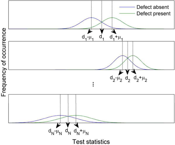
Illustration of linear observer test statistic distributions for the N sub-ensembles before shifting.

Suppose the test statistic distributions for the jth sub-ensemble are shifted by Δd_j, where Δd_j is independent of the input data, g. Denote c_j ≡ d_j + Δd_j. Then, as proven in Appendix B, when c_j = c₁(∀ j ∈ [2, N]), i.e. that test statistic distributions under the two classes cross at the same test statistic value for all the different sub-ensembles, as shown in Fig. 2, the pooled test statistics from the N sub-ensembles achieve the highest AUC.

Fig. 2.

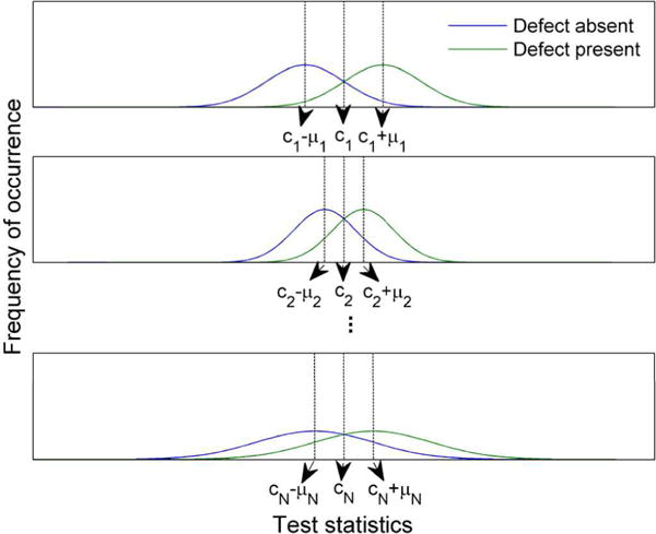
Illustration of linear observer test statistic distributions for the N sub-ensembles after shifting.

Theorem 2

When the sub-ensembles of data are MVN distributed and homoscedastic, if the LD is used to generate the test statistics for each sub-ensemble, the distributions of the test statistics under the two hypotheses for all sub-ensembles cross at test statistic λ = 0.

Rephrasing theorem 2 mathematically, for the jth sub-ensemble, when $\mathrm{\Delta }{d}_j=\frac{1}{2}\left({\overline{\mathbf{g}}}_{j0}^{\mathbf{T}}{\mathbf{K}}_{\mathbf{g}j}^{-\mathbf{1}}{\overline{\mathbf{g}}}_{j0}-{\overline{\mathbf{g}}}_{j1}^{\mathbf{T}}{\mathbf{K}}_{\mathbf{g}j}^{-\mathbf{1}}{\overline{\mathbf{g}}}_{j1}\right)$ as defined by (6)), where ${\overline{\mathbf{g}}}_{ji}$ and K_{g j} are, respectively, the mean data vector and covariance matrix of the data under hypothesis H_i(i = 0,1), then c_j = 0. In other words, the LD accomplishes the alignment of the test statistic distributions of different sub-ensembles shown in Fig. 2. This theorem is proved in Appendix C.

From Theorems 1 and 2, we can conclude that when the input ensemble of data vectors can be separated into sub-ensembles that are MVN and homoscedastic, and if only shifting of the HO test statistics by a different constant for each sub-ensemble is allowed prior to pooling them, then using the proposed multi-template LD strategy maximizes the AUC.

III. Methods

A. Phantom Design and Projection Data Simulation

To demonstrate the utility of the strategy in a realistic and clinically relevant setting, we used projection data from a previously-developed XCAT phantom population modeling dual-isotope MPS imaging [41]. The population included a total of 54 adult anatomies: 2 genders, 3 body core sizes, 3 heart sizes, and 3 thicknesses of subcutaneous adipose tissue. We modeled 6 defect types including 2 defect locations in the myocardium, anterior and inferior, with 3 severity (defect to normal myocardium activity ratio) and extent (volume percentage of the myocardial defect) combinations. The defect parameters are summarized in Table I (from Table II in [42]), and sample images of each defect type are shown in Fig. 3. Note that in all cases the product of the extent and severity was constant, representing a constant total reduction in myocardial uptake. An extent of 5% or severity of 10% represents difficult clinically relevant tasks. Note that in this paper, the same defect type implies that two defects are from the same location, have the same relative activity in comparison to the uptake in the corresponding myocardium, and the same relative volume in comparison to the volume of the myocardium. Since the sizes of and uptakes in the myocardium are different for different patients in the population, the absolute values of the activity and volume of the defect are different for different patients with the same defect type.

TABLE I.

Defect Parameters

Defect type	Location	Extent (%)	Severity (%)
1	Anterior	5	50
2	Inferior	5	50
3	Anterior	10	25
4	Inferior	10	25
5	Anterior	25	10
6	Inferior	25	10

Fig. 3.

Sample images of six defect types 1–6 (from left to right) from the short axis view of myocardium, red arrows indicate defect locations.

Low-noise projections were generated using the SimSET Monte Carlo code [43] and the angular response function method [44] for various organs (heart, liver, lung, blood pool, gall bladder, kidney, and background). The projections were scaled to a count level corresponding to injected activities of 10 mCi of Tc-99m sestamibi and 2 mCi of Tl-201, which are among the optimal injected activities suggested in [45]. The acquisition energy windows were 20% centered at 140.5keV for Tc-99m and 28% centered at 72keV for Tl-201. Attenuation, scatter, collimator-detector response and crosstalk between the two isotopes were modeled. The projections were generated at 60 views over 180° from left posterior oblique to right anterior oblique modeling a body-contouring orbit and a low-energy high-resolution collimator. The projection bin size was 0.442 cm. A total of 20 random uptake realizations each for Tc-99m and Tl-201, based on organ uptake distributions obtained from patient data, were generated for each anatomy by appropriately scaling the organ projections. Poisson noise was then added to the projection images. A more detailed description of the generation of the projection data is in [41].

B. Reconstruction and Post-processing

Images were reconstructed using the ordered subsets-expectation maximization (OS-EM) [46] algorithm with compensation for attenuation, collimator-detector response, scatter, and crosstalk contamination between projection data from the two radionuclides. Scatter compensation was based on the effective source scatter estimation (ESSE) method [47]. For each isotope, we used the true noise-free crosstalk projection data from the other in the crosstalk compensation, modeling an ideal crosstalk compensation method. We used four subsets per iteration for both Tc-99m and Tl-201 and evaluated images obtained after iterations 1, 2, 3, 5, 7, 10, 15, 20, 30, 45 and 60 for Tc-99m and 1, 2, 3, 5, 7, 10, 15 and 20 for Tl-201. After reconstruction, images were filtered using a Butterworth filter of order 8 and cutoff frequencies 0.08, 0.1, 0.12, 0.14, 0.16, 0.2 and 0.24 pixels⁻¹. The filtered images were then reoriented to short axis slices. A 64×64 image having the centroid of the defect at the center of the image was extracted, windowed so that the range [0, the maximum in the heart] was mapped to the range [0, 255], truncated to integers, and used in the observer studies.

C. Implementation and Evaluation of Observer Strategies

We evaluated three observer strategies by applying them to optimize the reconstruction parameters for this dual-isotope MPS study.

The first strategy was a conventional computationally-inexpensive HO strategy that used a single HO template for the entire ensemble. This strategy is referred to as the single-template HO strategy. The implementation in this work was similar to that described in [19, 48]. First, feature vectors were calculated by applying six rotationally symmetric frequency channels. The first channel had a starting frequency and channel width of 1/128 cycles per pixel. Subsequent channels abutted the previous one and had double the previous width. We calculated the HO test statistics using a leave-one-out technique [19, 49]. In that technique, the HO was trained on an ensemble including all data except a single image. The resulting HO template was then applied to the remaining image to calculate a single test statistic. For each combination of iteration number and cutoff frequency, a single test statistic was calculated with 6,480 pairs of defect-present and -absent images (12,959 training images to estimate the template and 1 testing image as the input image data). This process was repeated with each image in the ensemble left out in turn, resulting in a number of test statistics equal to 12,960. ROC analysis [50] using the LABROC code [51] was then applied to this set of test statistics to estimate the AUC.

The other two strategies were the two multi-template strategies described in II.B and II.C. We first divided the dataset into multiple sub-ensembles, where each sub-ensemble had the same defect type. As explained above, the absolute value of the defect volumes and uptakes were different in a sub-ensemble, leading to an SKS dataset. However, since the absolute activity in each organ was sampled from a relatively continuous distribution, and the organ volume was relatively continuous, the signal and background variations in each sub-ensemble were sampled from a relatively continuous distribution. Thus, based on the observations in [20], we expected each SKS sub-ensemble to have an approximately MVN distribution. This agreed with empirical observations in this study, as shown in Fig. 4. Note that the entire ensemble had a multi-modal distribution. However, the sub-ensemble following the above partitioning strategy was approximately normally distributed.

Fig. 4.

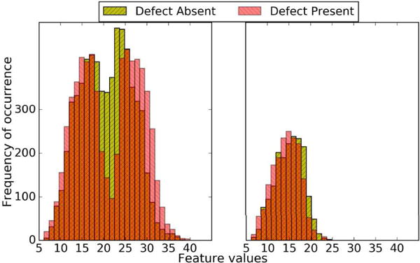
Thirty bin histograms of the first channel feature value distribution for the entire ensemble (left) and for the SKS sub-ensemble corresponding to defect type 1, which contains the full mixture of anatomies present in the whole patient population (right) for Tc images at iteration number 5 (4 subsets/iteration) and cutoff frequency 0.1 pixel⁻¹.

We also tested the homoscedasticity, i.e. the equality of the covariance matrix under the defect absent and defect present cases, for each of the sub-ensembles. Sample images of covariance matrices under the two hypotheses for the six sub-ensembles are shown in Fig. 5. Visually, the homoscedasticity condition was approximately satisfied. We also tested the homoscedasticity condition based on two metrics defined in (1) and (2). The CMD values for all sub-ensembles and all reconstruction parameters for Tc and Tl are summarized in Table II. The mean CMD for all sub-ensembles and all reconstruction parameters was close to 0, which indicated good similarities between the two covariance matrices up to a scale. The determinant ratio values for all sub-ensembles and all reconstruction parameters for Tc and Tl are summarized in Table III. Since the mean of this determinant ratio was very close to 1, the average scale difference between the two covariance matrices for each sub-ensemble was small.

Fig. 5.

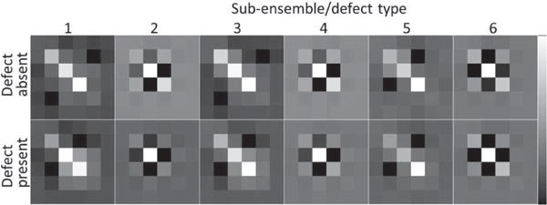
Covariance matrices under the two hypotheses (top row: defect-absent, bottom row: defect-present) for the six sub-ensembles (the 1st to the 6th columns are corresponding to defect type 1 to 6, respectively) for Tc images at iteration number 5 (4 subsets/iteration) and cutoff frequency 0.1 pixel⁻¹.

TABLE II.

Mean, minimum, and Maximum CMD for all sub-ensembles and all reconstruction parameters

	Mean	Minimum	Maximum
Tc	0.0293	0.0004	0.1488
Tl	0.0144	0.0005	0.0602

TABLE III.

Mean, minimum, and maximum determinant ratio for all sub-ensembles and all reconstruction parameters

	Mean	Minimum	Maximum
Tc	1.25	1.01	2.19
Tl	1.08	1.01	1.25

Based on the above, we concluded the sub-ensembles were approximately homoscedastic. Thus, using this partitioning strategy based on defect types yielded sub-ensembles that approximately satisfied the MVN and homoscedasticity condition. The results in IV.A also empirically indicate this.

For the multi-template LD with pooled test statistics strategy, we estimated the LD test statistics using the above leave-one-out strategy for each sub-ensemble. The resulting sets of test statistics from all the sub-ensembles were pooled and used to compute the overall AUC. Thus, the ROC analysis was performed only once.

For the multi-template HO with averaged AUCs strategy, HO test statistics were obtained using the above leave-one-out strategy, the AUC was computed for each sub-ensemble, and the weighted sum of the AUCs for all sub-ensembles was calculated, where the weight was the fraction of cases in each sub-ensemble.

For each sub-ensemble and each combination of iteration number and cutoff frequency, a single test statistic was calculated with 1,080 pairs of defect-present and -absent images (2,159 training images and 1 testing image) for the two multi-template strategies.

A diagram illustrating the three observer strategies is shown in Fig. 6.

Fig. 6.

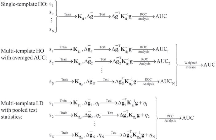
Diagram illustrating the data flow for the three observer strategies investigated. Sj stands for the jth sub-ensemble (1≤j≤N), where N is the total number of sub-ensembles. $\mathrm{\Delta }{\overline{g}}_{\mathbf{j}}$, K_gj, and η_j denote the mean data vector, the covariance matrix of the data, and the term defined in Equation (6) for the jth sub-ensemble, respectively.

The overall goal was to optimize the number of iterations of the OS-EM algorithm and the cutoff frequency of the post-reconstruction-low-pass-filter for Tc and Tl images. For all three strategies, the reconstruction parameters that achieved the highest AUC values for the entire ensemble were deemed optimal.

IV. Results

A. Effect of Using the LD Observer Instead of the HO Observer for Multiple Sub-ensembles

The effect of using the LD instead of the HO for the six sub-ensembles obtained using the partitioning method in III.C can be seen in Figs. 7 and 8. Fig. 7 shows the test statistic distributions for the six different sub-ensembles using the HO. We observed that the ranges of the test statistic values for different sub-ensembles were different. The distributions for the LD are shown in Fig. 8. Note that the histograms of test statistic of the two classes for all sub-ensembles cross when the value of the test statistic is approximately zero (not strictly zero because the feature vectors in each sub-ensemble were not strictly MVN distributed and homoscedastic, and the histograms were generated from a finite number of samples). This indirectly indicates that sub-ensembles obtained using the partitioning method based on defect type in this study approximately satisfy the MVN and homoscedasticity condition.

Fig. 7.

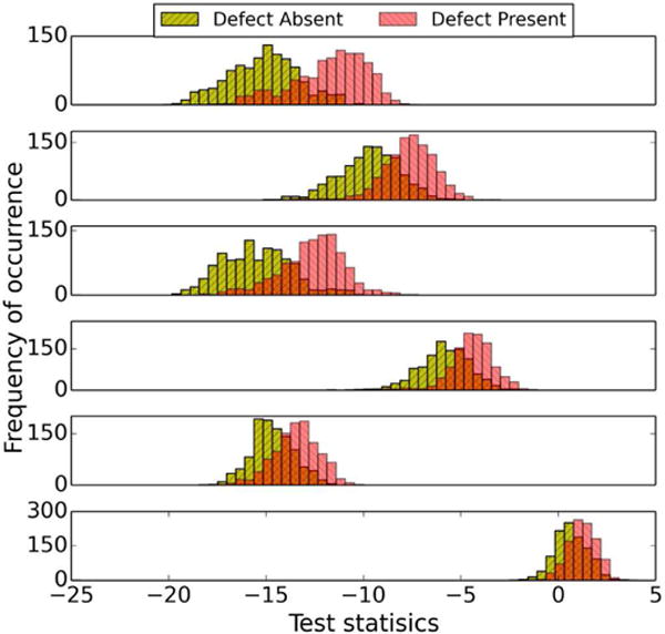
Sixty-four bin histograms of HO test statistics for different defect types for Tc at iteration number 1 (4 subsets/iteration) and cutoff frequency 0.1 pixel⁻¹. The graphs, from top to bottom, are for defect types 1–6, respectively.

Fig. 8.

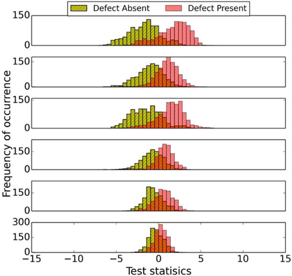
Sixty-four bin histograms of LD test statistics for different defect types for Tc at iteration number 1 (4 subsets/iteration) and cutoff frequency 0.1 pixel⁻¹. The graphs, from top to bottom, are for defect types 1–6, respectively

B. Comparison of the AUCs Using the Three Observer Strategies

For each set of reconstruction parameters, we computed AUC values using the three observer strategies. The calculated AUC was highest for the multi-template LD with pooled test statistics strategy and lowest for the conventional single-template HO strategy for all the sets of reconstruction parameters investigated. The mean, minimum, and maximum of the differences in the AUC values over all reconstruction parameters between the multi-template LD with pooled test statistics strategy and single and multi-template HO strategy and between the two multi-template strategies for Tc and Tl images are summarized in Tables IV and V, respectively. The differences between the multi-template strategies and single-template HO strategy are not surprising because the signal uncertainty in the entire dataset was larger than in the sub-ensembles.

TABLE IV.

Differences Between AUC Values for the Multi-template LD with Pooled Test Statistics and Single-Template HO Strategies

	Mean	Minimum	Maximum
Tc	0.054±0.005	0.033±0.004	0.082±0.005
Tl	0.029±0.006	0.024±0.006	0.042±0.006

The values after ± are the standard deviations of the AUCs.

TABLE V.

Differences Between AUC Values for the Multi-template LD with Pooled Test Statistics and Multi-Template HO with averaged AUCs Strategies

	Mean	Minimum	Maximum
Tc	0.025±0.004	0.005±0.006	0.038±0.005
Tl	0.015±0.006	0.003±0.006	0.023±0.006

The values after ± are the standard deviations of the AUCs.

The AUC values obtained using the optimal parameters for each observer strategy are shown in Fig. 9. Note that the multi-template LD with pooled test statistics strategy gave the highest AUC value of the three strategies. The p-values for a two-tailed t-test of the differences between the three strategies estimated using bootstrapping were smaller than 0.05 for both Tc and Tl, indicating that the differences were statistically significant. The differences in the AUC values between the strategies were all greater than 0.01. We considered a difference of 0.01 in the AUC to be clinically important, since the AUC differences for images reconstructed with and without scatter or detector response compensation were 0.01 in similar studies [52], and these combinations of compensations have been adopted and recognized as clinically significant. The differences between the three strategies were larger for Tc than Tl because the optimal parameters obtained by the three observer strategies were more different for Tc and more similar for Tl, as shown in Section IV.C.

Fig. 9.

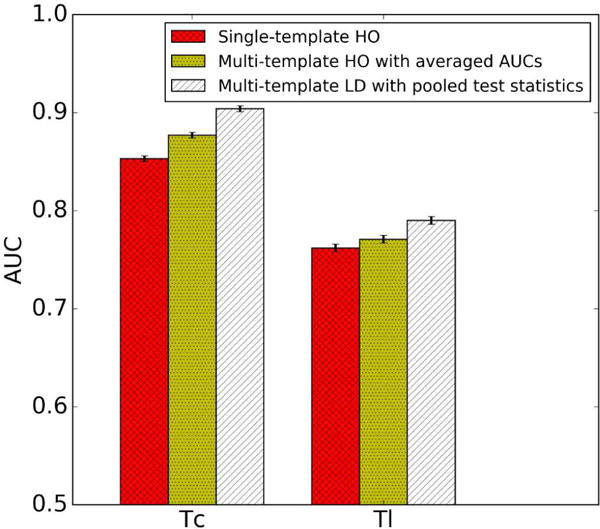
AUC values with the optimal parameters obtained by three observer strategies.

C. Comparison of the Optimal Parameters Obtained by the Three Observer Strategies

The optimal parameters for the entire dataset obtained by the three different observer strategies are shown in Fig. 10 for Tc (left) and Tl (right). In these plots, the cross shows the parameter set that gave the highest AUC values; the filled circles show sets of parameters where the difference in AUC values with respect to the optimal one were not statistically significant (p-value > 0.05); the contour line surrounds combinations of parameters for which the AUC values differed by 0.01 or less. Parameter combinations inside this curve were considered to be near-optimal.

Fig. 10.

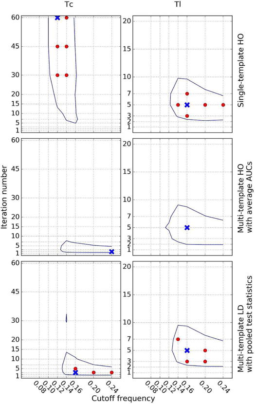
Optimal parameters for all defect types for Tc (left) and Tl (right) using (top to bottom): single-template HO, multi-template HO with averaged AUCs, and multi-template LD with pooled test statistics strategies. The crosses represent the set of parameters that achieved the maximum AUC. The filled circles represent the parameter points where the difference in AUC with respect to the maximum AUC was not statistically significant. The contour line indicates the region where AUC values differed from the optimal one by no more than 0.01, a difference considered clinically important. We used 4 subsets/iteration during the OS-EM reconstructions.

For Tc, the two multi-template observer strategies were optimal for lower iteration numbers and higher cutoff frequencies than with the conventional HO strategy. One explanation is that a higher iteration number, which improves image resolution, is preferred by the single-template HO strategy when there is more background variability since higher resolution tends to reduce the effects on myocardial intensity of variations in anatomy and uptake in neighboring organs; a lower cutoff frequency was needed to reduce the noise when the iteration number was high.

For Tl, the near-optimal parameter ranges using the three observer strategies were similar. This was different than for Tc and can be explained as follows. The observer templates for the three strategies would be the same when the distributions of feature vector values were the same for different sub-ensembles. The positions of the feature vector distributions were largely determined by the pixel values near the defect position. For the anterior defect, this was largely the myocardium, as activity in neighboring structures was small. For the inferior defect, the liver also made a significant contribution because of its high uptake and proximity to the defect. Assuming that the contribution to the feature vector values from the myocardium in the two locations was the same, the positions of the feature vector distributions for an anterior compared to an inferior defect were determined largely by the liver contribution. The activity in the liver relative to the myocardium for Tc was greater than for Tl by a factor of 1.29. Thus, there was a greater absolute shift in the positions of the feature vector distributions for Tc for the anterior versus inferior defect locations, as seen in Fig. 11. The conventional HO observer is more sensitive to differences in the positions of the distributions of test statistics from the two locations, for reasons described above. Thus the conventional HO strategy would be more different from the other two observers for Tc than for Tl, resulting in the possibility of differences in the optimal parameter combinations.

Fig. 11.

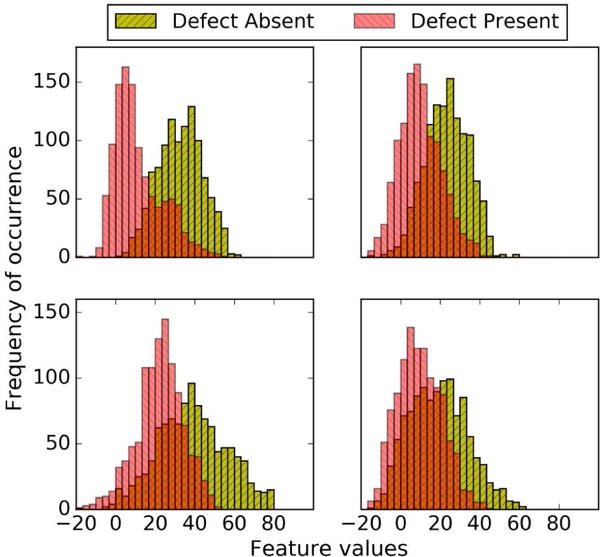
Thirty bin feature vector histograms of Channel 4 outputs for Tc (left) and Tl (right) for defect types 1 (top, anterior defect with 5% extent and 50% severity) and 2 (bottom, inferior defect with 5% extent and 50% severity) using 5 iterations (4 subsets/iteration) and a cutoff frequency of 0.1 pixel⁻¹.

Note that a similar argument applies to the different defect types at the same location. In this case, the differences in the positions of the feature vector distributions were a function of the uptake in the myocardium. Since the myocardium had a Tc activity that was greater by a factor of 1.97 than Tl, the absolute difference in the positions of the feature vector distributions would be greater for Tc than for Tl. The conventional HO strategy would have greater difficulty dealing with this larger difference, and thus there would be a greater difference for the single-template strategy compared to the other two observers for Tc than for Tl.

To determine which observer strategy gave the truly optimal parameters for the combination of all defect types, we compared the performance for each defect type using the optimal parameters obtained by the three observer strategies. The optimal parameters obtained by each strategy are shown by the crosses in Fig. 10. Note that for each sub-ensemble (corresponding to each defect type in this study), the AUCs in Table VI were calculated using the single-template HO strategy, since the data in each sub-ensemble were approximately MVN and homoscedastic. The results are shown in Table VI. For each defect type, the AUC values obtained with the optimal parameters from the multi-template LD with pooled test statistics strategy were always greater than or equal to the AUCs obtained using parameters optimal for the conventional HO strategy. The largest differences in AUC values between the multi-template and the single-template strategies were for defect types 5 and 6, the defects with the largest extent and lowest severity. This is likely because detecting defect types 1–4, which had higher contrasts, was easier (as shown in Fig. 3), and the AUC was thus less sensitive to changes in the reconstruction parameters. The AUC values for the two multi-template strategies were comparable: for some defect types (defect types 1, 5, 6), the multi-template LD strategy gave higher AUCs, but not for other defect types; for all mixed defect types, the two multi-templates strategies were comparable (as shown in Fig. 10), the optimal parameters obtained by the two multi-template strategies were within the optimal parameter ranges of each other.

TABLE VI.

Comparison of AUCs for Tc for Individual Sub-ensemble Using the Optimal Parameters Obtained Using the Three Observer Strategies

Sub-ensemble/defect type	Single-template HO	Multi-template HO with averaged AUCs	Multi-template LD with pooled test statistics
1	0.968±0.003	0.980±0.002	0.977±0.003
2	0.949±0.004	0.937±0.005	0.949±0.004a
3	0.954±0.004	0.950±0.004a	0.957±0.004a
4	0.899±0.006	0.877±0.007	0.900±0.006a
5	0.709±0.011	0.793±0.009	0.774±0.010
6	0.674±0.011	0.724±0.011	0.702±0.011

The AUC for each sub-ensemble was calculated using the single-template HO strategy and values after ± are the standard deviations of the AUCs.

^aThe AUC difference compared to the single-template strategy was either not statistically significant (p > 0.05) or not clinically important (difference < 0.01).

V. Discussion

We have developed and evaluated two multi-template strategies to classify non-MVN distributed data using a sub-ensemble-based approach. In order to use either of them to rank different systems in place of human observers, correlation of task performance calculated by these model observers and human performance on the corresponding task must be studied.

An important observation in this study was that good correlation of different model observers in a one-dimensional parameter space did not imply good correlation in a multidimensional parameter space. More specifically, in this study, we were optimizing two reconstruction parameters: the iteration number of the OS-EM algorithm and the cutoff frequency of a post reconstruction low-pass filter. We observed that the three observer strategies had very good correlations when comparing only the ranking of different values for one parameter with the other parameter fixed, as shown in Figs 12 and 13. However, the three strategies achieved different optimal parameters when we simultaneously optimized both parameters, as shown in Fig. 10. This happens when the ranking of different values for one parameter changes with the other parameter(s). The result is significant since it implies that the correlation of different observers in a one-dimensional parameter space, as studied previously [16, 23, 24], may not indicate the correlation in a multi-dimensional parameter space.

Fig. 12.

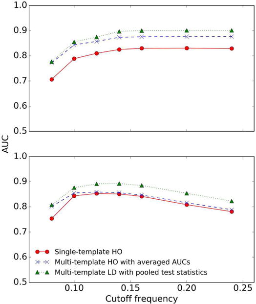
AUC plot for Tc of three observer strategies for different cutoff frequencies (pixel⁻¹) at iterations 2 (upper) and 60 (lower). We used 4 subsets/iteration during the OS-EM reconstructions.

Fig. 13.

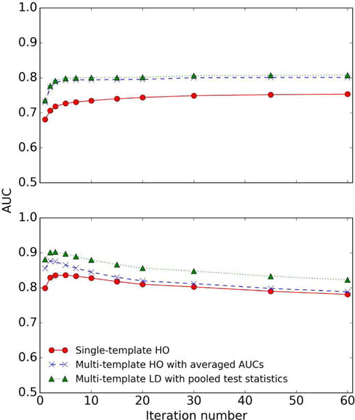
AUC plot for Tc of three observer strategies for different iteration numbers at cutoff frequencies 0.08 (upper) and 0.24 (lower) pixel-1. We used 4 subsets/iteration during the OS-EM reconstructions.

An unresolved question is the relative merit of the two multi-template strategies. In terms of AUCs, the multi-template LD with pooled test statistics strategy provided higher values. In terms of optimal parameter range, the two strategies obtained similar optimal parameter ranges for the data used in this study. However, it is possible that differences in ranking of different image systems could be observed for other tasks, and this remains a topic where a future investigation is required.

One advantage of the multi-template LD with pooled test statistics strategy is that it requires fewer ROC analysis operations compared to the multi-template HO with averaged AUCs strategy. This could be important when there are a small number of cases available for certain sub-ensembles since AUC estimation methods are often not reliable for a small number of cases. The effect of having only a small number of cases on the performance of the two multi-template strategies is another topic requiring investigation.

In addition, the multi-template LD with pooled test statistics strategy is also more theoretically sound for the following reason. For the multi-template HO with averaged AUCs strategy, the AUC values for each defect type are averaged to give the overall AUC value, which is equivalent to averaging the ROC curves to give an overall ROC curve. This is equivalent to averaging true positive fraction (TPF) values at the same false positive fraction (FPF) value. However, the exact meaning of averaging the TPFs for a given FPF is difficult to define, since the FPF values for different ROC curves arise from different decision threshold values. Thus, the meaning of averaged ROC curves is not clear. For the multi-template LD with pooled test statistics strategy, the pooling of the test statistics is justified based on pooling of the likelihood ratios and the fact that the shifting provided by the LD gives the maximum overall AUC; a single ROC curve is estimated for the entire ensemble of test statistics, thus avoiding the questionable averaging of ROC curves used by the multi-template HO strategy.

An area requiring future work is the development of general methods to partition the data into MVN and homoscedastic sub-ensembles. In this paper, we described two feasible methods based on knowing characteristics of the variations of the signal and background. The first method is to partition the data into SKE sub-ensembles. This method is general, but can be impractical if there are large numbers of signal variations. The second method, and the one investigated in this work, was to partition the data into SKS sub-ensembles with signal variations that were small in comparison to background variations, and with signal and background variations sampled from a relatively continuous distribution. Other partition methods undoubtedly exist and may be needed for other applications. One potentially general approach is to use data-centric methods to form the ensembles. For example, clustering-based techniques have been proposed for image segmentation [53, 54]. These methods treat the data as a Gaussian mixture model to partition the data into individual Gaussian components. A similar technique could be developed to partition non-MVN channel-output data. Such an approach would be easier in the channel output domain since the number of channels is far smaller than the number of voxels in images where this clustering approach has been used for segmentation. As observed above, the non-MVN data in our experiments could be treated as a Gaussian mixture model, and thus a clustering approach like this would likely be appropriate.

An important question is what values of CMD and the determinant ratio are small enough to indicate sufficient homoscedasticity of the sub-ensembles in this study. The results in Section IV indirectly indicate that the homoscedasticity condition is satisfied sufficiently well with the values of the CMD and determinant ratio observed in this study. Thus, a CMD value of 0.03 and a determinant ratio of 1.25 may be regarded as a sufficient condition in similar studies. Whether these thresholds are sufficient in all cases or whether other values would have been acceptable has not been addressed in this work. Detailed studies of the necessary levels of CMD and determinant ratio to provide homoscedasticity are needed.

It must also be emphasized that the investigated multi-template strategies are general strategies to handle non-MVN data, and are not limited to feature vectors generated using the anthropomorphic channels evaluated in this paper. The advantages of the strategies apply to other potentially non-MVN data, such as feature vectors from other anthropomorphic or efficient channels or even projection data. These multi-template strategies are also less computationally expensive when the number of sub-ensembles is much smaller than the possible number of signal types compared to the previous multi-template strategies for SKS and SKEV tasks.

VI. Conclusion

We have proposed a novel multi-template linear observer strategy for analyzing detection performance in datasets that are not MVN distributed. The strategy consists of dividing the data into sub-ensembles that are MVN and homoscedastic, applying different Linear Discriminant (LD) templates on the different sub-ensembles, and finally pooling the test statistics. We also adapted another multi-template strategy, initially proposed in the context of SKEV tasks, for non-MVN distributed data based on the sub-ensemble approach. Both of these multi-template strategies were compared to the conventional single-template HO strategy. The strategies were compared by applying them to optimize reconstruction parameters for the non-MVN data from a realistic simulated myocardial perfusion SPECT dataset. The two multi-template strategies yielded more optimal reconstruction parameters compared to the single-template HO strategy in terms of higher AUC for each sub-ensemble. The novel multi-template LD with pooled test statistics strategy is more theoretically justified and provided a higher AUC for the entire ensemble than the adapted multi-template strategy. The theory and results we presented provide strong evidence in favor of using the proposed multi-template LD strategy to classify non-MVN data such as that arising from the clinically realistic task with background and signal variations used in this study.

Appendix A

Here we prove the homoscedasticity condition will be approximately satisfied if the signal variations are relatively small compared to the background variations and the signal and background are uncorrelated.

Suppose B and S are the vectors of background and signal data. The covariance matrices of B and S are expressed in the following two equations:

$${\mathbf{K}}_{\mathbf{B}}=E\left[\left(\mathbf{B}-E\left[\mathbf{B}\right]\right){\left(\mathbf{B}-E\left[\mathbf{B}\right]\right)}^T\right],$$ (A1)

$${\mathbf{K}}_{\mathbf{S}}=E\left[\left(\mathbf{S}-E\left[\mathbf{S}\right]\right){\left(\mathbf{S}-E\left[\mathbf{S}\right]\right)}^T\right],$$ (A2)

where E[.] denotes the expectation of the corresponding vector or matrix.

The covariance matrix of B+S is expressed as

$$\begin{array}{l}{\mathbf{K}}_{\mathbf{B}+\mathbf{S}}=E\left[\left(\mathbf{B}+\mathbf{S}-E\left[\mathbf{B}+\mathbf{S}\right]\right){\left(\mathbf{B}+\mathbf{S}-E\left[\mathbf{B}+\mathbf{S}\right]\right)}^T\right]\\ ={\mathbf{K}}_{\mathbf{B}}+{\mathbf{K}}_{\mathbf{S}}+E\left[\left(\mathbf{B}-E\left[\mathbf{B}\right]\right){\left(\mathbf{S}-E\left[\mathbf{S}\right]\right)}^T\right]\\ +E\left[\left(\mathbf{S}-E\left[\mathbf{S}\right]\right){\left(\mathbf{B}-E\left[\mathbf{B}\right]\right)}^T\right].\end{array}$$ (A3)

When B and S are not correlated, we have

$$\begin{array}{l}E\left[\left(\mathbf{B}-E\left[\mathbf{B}\right]\right){\left(\mathbf{S}-E\left[\mathbf{S}\right]\right)}^T\right]\\ =E\left[\left(\mathbf{S}-E\left[\mathbf{S}\right]\right){\left(\mathbf{B}-E\left[\mathbf{B}\right]\right)}^T\right]=0.\end{array}$$ (A4)

Based on (A3) and (A4),

$${\mathbf{K}}_{\mathbf{B}+\mathbf{S}}={\mathbf{K}}_{\mathbf{B}}+{\mathbf{K}}_{\mathbf{S}}.$$ (A5)

When K_S ≪ K_B, K_B+S ≈ K_B, which means the covariance matrices of the background with and without the signal are approximately equal if the signal variations are relatively small compared to the background variations and if the signal and background are uncorrelated.

Appendix B

Here we prove Theorem 1 in II.C.

Let t be the decision threshold. For the jth sub-ensemble, the true-positive fraction (TPF) and false-positive fraction (FPF) can be expressed as

$$TP{F}_j\left(t\right)={\displaystyle \underset{t}{\overset{\mathrm{\infty }}{\int }}\frac{1}{\sqrt{2\pi }{\sigma }_j}}\exp \left[-\frac{{\left(\lambda -c_j-{\mu }_j\right)}^2}{2{\sigma }_j^2}\right]d\lambda$$ (B1)

and

$$FP{F}_j\left(t\right)={\displaystyle \underset{t}{\overset{\mathrm{\infty }}{\int }}\frac{1}{\sqrt{2\pi }{\sigma }_j}}\exp \left[-\frac{{\left(\lambda -c_j+{\mu }_j\right)}^2}{2{\sigma }_j^2}\right]d\lambda ,$$ (B2)

where λ is the test statistic value.

Let P_j be the prevalence of the jth sub-ensemble. If we pool the test statistics from all sub-ensembles we obtain

$$\mathit{TPF}\left(t\right)={\displaystyle \sum _{j=1}^N{P}_j}\times TP{F}_j\left(t\right)$$ (B3)

and

$$\mathit{FPF}\left(t\right)={\displaystyle \sum _{j=1}^N{P}_j}\times FP{F}_j\left(t\right).$$ (B4)

Note that

$${\displaystyle \sum _{j=1}^N{P}_j}=1$$ (B5)

Using the definition of the error function [55]

$$\frac{2}{\sqrt{\pi }}{\displaystyle \underset{z}{\overset{\mathrm{\infty }}{\int }}\exp \left(-t^2\right)}dt=1-\mathit{erf}\left(z\right),$$ (B6)

and equations (B1)–(B4), we have

$$\mathit{TPF}\left(t\right)={\displaystyle \sum _{j=1}^N\frac{P_j}{2}}\left[1-\mathit{erf}\left(\frac{t-c_j-{\mu }_j}{\sqrt{2}{\sigma }_j}\right)\right]$$ (B7)

and

$$\mathit{FPF}\left(t\right)={\displaystyle \sum _{j=1}^N\frac{P_j}{2}}\left[1-\mathit{erf}\left(\frac{t-c_j+{\mu }_j}{\sqrt{2}{\sigma }_j}\right)\right].$$ (B8)

According to the definition of the AUC [31]

$$\mathit{AUC}=-{\displaystyle \underset{-\mathrm{\infty }}{\overset{\mathrm{\infty }}{\int }}\mathit{TPF}}\left(t\right)\frac{\mathit{dFPF}}{dt}dt.$$ (B9)

Using equations (B7)–(B9) and the following property of the error function [55]

$$\frac{d}{dz}\mathit{erf}\left(z\right)=\frac{2}{\sqrt{\pi }}\exp \left(-z^2\right),$$ (B10)

we can write the AUC as

$$\begin{array}{l}\mathit{AUC}\left(c_2,c_3,\cdots ,c_N\right)\\ ={\displaystyle \underset{-\mathrm{\infty }}{\overset{\mathrm{\infty }}{\int }}\left\{{\displaystyle \sum _{j=1}^N\frac{P_j}{2}}\left[1-\mathit{erf}\left(\frac{t-c_j-{\mu }_j}{\sqrt{2}{\sigma }_j}\right)\right]\right\}}\\ \times \left\{{\displaystyle \sum _{i=1}^N\frac{P_i}{\sqrt{2\pi }{\sigma }_i}\exp \left[-{\left(\frac{t-c_i+{\mu }_i}{\sqrt{2}{\sigma }_i}\right)}^2\right]}\right\}dt,\end{array}$$ (B11)

where we have written the AUC as a function of c₂, c₃,⋯, c_N, since we are interested in finding the values of c₂, c₃,⋯, c_N that maximize the AUC.

Using (B5) and expanding the terms in (B11), we can write the AUC as

$$\begin{array}{l}\mathit{AUC}\left(c_2,c_3\cdots ,c_N\right)\\ =\frac{1}{2}{\displaystyle \underset{-\mathrm{\infty }}{\overset{\mathrm{\infty }}{\int }}{\displaystyle \sum _{i=1}^N\frac{P_i}{\sqrt{2\pi }{\sigma }_i}}\exp \left[-{\left(\frac{t-c_i+{\mu }_i}{\sqrt{2}{\sigma }_i}\right)}^2\right]}dt\\ -\frac{1}{2\sqrt{2\pi }}{\displaystyle \sum _{j=1}^N\frac{P_j^2}{{\sigma }_j}}{\displaystyle \underset{-\mathrm{\infty }}{\overset{\mathrm{\infty }}{\int }}\mathit{erf}}\left(\frac{t-c_j-{\mu }_j}{\sqrt{2}{\sigma }_j}\right)\\ \times \exp \left[-{\left(\frac{t-c_j+{\mu }_j}{\sqrt{2}{\sigma }_j}\right)}^2\right]dt\\ -\frac{1}{2\sqrt{2\pi }}{\displaystyle \sum _{j=1}^N{\displaystyle \sum _{i=1,i\ne j}^N\frac{P_j{P}_i}{{\sigma }_i}}}{\displaystyle \underset{-\mathrm{\infty }}{\overset{\mathrm{\infty }}{\int }}\mathit{erf}}\left(\frac{t-c_j-{\mu }_j}{\sqrt{2}{\sigma }_j}\right)\\ \times \exp \left[-{\left(\frac{t-c_i+{\mu }_i}{\sqrt{2}{\sigma }_i}\right)}^2\right]dt.\end{array}$$ (B12)

Note that the first and second terms in the above can be made independent of the constants c₂, c₃,⋯, c_N by a change of variables. For example, in the first term, we could simply replace t − c_i by t′. Thus, these terms can be ignored when maximizing the AUC. Denoting the last term by k (c₂, c₃,⋯, c_N), we have:

$$\begin{array}{l}k\left(c_2,c_3\cdots c_N\right)\\ =-\frac{1}{2\sqrt{2\pi }}{\displaystyle \sum _{j=1}^N{\displaystyle \sum _{i=1,i\ne j}^N\frac{P_j{P}_i}{{\sigma }_i}}}{\displaystyle \underset{-\mathrm{\infty }}{\overset{\mathrm{\infty }}{\int }}\mathit{erf}}\left(\frac{t-c_j-{\mu }_j}{\sqrt{2}{\sigma }_j}\right)\\ \times \exp \left[-{\left(\frac{t-c_i+{\mu }_i}{\sqrt{2}{\sigma }_i}\right)}^2\right]dt.\end{array}$$ (B13)

Replacing $\frac{t-c_j-{\mu }_j}{\sqrt{2}{\sigma }_j}$ by t′, and using the following property of the error function [55]

$${\displaystyle \underset{-\mathrm{\infty }}{\overset{\mathrm{\infty }}{\int }}\mathit{erf}}\left(x\right)\exp \left[-{\left(ax+b\right)}^2\right]dx=-\frac{\sqrt{\pi }}{a}\mathit{erf}\left(\frac{b}{\sqrt{a^2+1}}\right),$$ (B14)

we can write equation (B13) as

$$\begin{array}{l}k\left(c_2,c_3\cdots c_N\right)\\ =-\frac{1}{2}{\displaystyle \sum _{j=1}^N{\displaystyle \sum _{i=1,i\ne j}^N{P}_i{P}_j\mathit{erf}}}\left(\frac{{\mu }_j+c_j-c_j+{\mu }_i}{\sqrt{2\left({\sigma }_i^2+{\sigma }_j^2\right)}}\right).\end{array}$$ (B15)

Differentiating the above expression with respect to c₂, c₃,⋯, c_N and equating the result to zero yields the critical points at which k (c₂, c₃,⋯, c_N), or alternatively, the AUC is maximized or minimized. Thus, differentiating the above expression with respect to any general c_I, where I = 2,…, N, yields

$$\begin{array}{l}\frac{\partial k\left(c_2,c_3,\cdots ,c_N\right)}{\partial c_I}\\ =\frac{1}{\sqrt{2\pi }}{\displaystyle \sum _{i=1,i\ne I}^N\frac{P_I{P}_i}{\sqrt{{\sigma }_I^2+{\sigma }_i^2}}}\{\exp \left[-{\left(\frac{c_I+{\mu }_I-c_i+{\mu }_i}{\sqrt{2\left({\sigma }_I^2+{\sigma }_i^2\right)}}\right)}^2\right]\\ -\exp \left[-{\left(\frac{c_i+{\mu }_i-c_I+{\mu }_I}{\sqrt{2\left({\sigma }_I^2+{\sigma }_i^2\right)}}\right)}^2\right]\}.\left(I=2.\dots ,N\right).\end{array}$$ (B16)

The above expression is equal to zero when the exponential terms are equal, which occurs when c_I = c₁(I = 2,…, N). In Appendix D, Hessian matrix of k (c₂, c₃,⋯,c_N) is proved to be strictly negative definite at any (c₂, c₃,⋯,c_N). Thus, when c_i = cj (∀i, j ∈ [1, N]), the term k (c₂, c_3,⋯,c_N), and hence the AUC, is maximized.

Appendix C

Here we prove theorem 2 in II.C.

For the jth sub-ensemble, assuming the input data are MVN distributed and homoscedastic, the probability distribution of the data vectors is

$$\begin{array}{l}pr\left(\mathbf{g}|H_i\right)=\frac{1}{{\left(2\pi \right)}^{M/2}\sqrt{|{\mathbf{K}}_{\mathbf{g}\mathrm{ j}}|}}\\ \times \exp \left[-\frac{1}{2}{\left(\mathbf{g}-{\overline{\mathbf{g}}}_{ji}\right)}^T{\mathbf{K}}_{\mathbf{g}j}^{-1}\left(\mathbf{g}-{\overline{\mathbf{g}}}_{ji}\right)\right].\left(i=0,1\right)\end{array}$$ (C1)

Then, from equation (C1), if $\mathbf{g}=\frac{{\overline{\mathbf{g}}}_{j0}+{\overline{\mathbf{g}}}_{j1}}{2}$, we can derive that pr (g|H₀) = pr (g|H₁), and pr (λ(g)|H₀) = pr (λ(g) H₁). This means that the distributions of the test statistics of the two hypotheses are equal (i.e., the test statistic distributions cross) when $\mathbf{g}=\frac{{\overline{\mathbf{g}}}_{j0}+{\overline{\mathbf{g}}}_{j1}}{2}$.

The LD test statistic defined by equation (4) at the point $\mathbf{g}=\frac{{\overline{\mathbf{g}}}_{j0}+{\overline{\mathbf{g}}}_{j1}}{2}$ is given by

$$c_j=\lambda \left(\mathbf{g}\right)=\mathrm{\Delta }{\overline{\mathbf{g}}}_j^{\mathbf{T}}{\mathbf{K}}_{\mathbf{g}j}^{-1}\mathbf{g}+\frac{1}{2}\left({\overline{\mathbf{g}}}_{j0}^{\mathbf{T}}{\mathbf{K}}_{\mathbf{g}j}^{-1}{\overline{\mathbf{g}}}_{j0}-{\overline{\mathbf{g}}}_{j1}^{\mathbf{T}}{\mathbf{K}}_{\mathbf{g}j}^{-1}{\overline{\mathbf{g}}}_{j1}\right)=0,$$ (C2)

where $\mathrm{\Delta }{\overline{\mathbf{g}}}_j=\overline{{\mathbf{g}}_{\mathbf{j}\mathbf{1}}}-{\overline{\mathbf{g}}}_{j0}$.

Now, we have shown that shifting the HO test statistics by the term $\mathrm{\Delta }{d}_j=\frac{1}{2}\left({\overline{\mathbf{g}}}_{j0}^{\mathbf{T}}{\mathbf{K}}_{\mathbf{g}j}^{-1}{\overline{\mathbf{g}}}_{j0}-{\overline{\mathbf{g}}}_{j1}^{\mathbf{T}}{\mathbf{K}}_j^{-1}{\overline{\mathbf{g}}}_{j1}\right)$ leads to the distributions of the test statistics being equal at the point where the test statistic is zero.

Appendix D

Here we prove that the Hessian matrix of k (c₂, c₃,⋯, c_N)is negative definite.

The Hessian matrix of k (c₂, c₃,⋯, c_N) is

$$\begin{array}{l}H=\\ {\left[\begin{array}{cccc}\frac{{\partial }^{2}k\left(c_2,c_3,\cdots ,c_N\right)}{\partial c_2^2}& \frac{{\partial }^{2}k\left(c_2,c_3,\cdots ,c_N\right)}{\partial c_2{c}_3}& \cdots & \frac{{\partial }^{2}k\left(c_2,c_3,\cdots ,c_N\right)}{\partial c_2{c}_N}\\ \frac{{\partial }^{2}k\left(c_2,c_3,\cdots ,c_N\right)}{\partial c_3{c}_2}& \frac{{\partial }^{2}k\left(c_2,c_3,\cdots ,c_N\right)}{\partial c_3^2}& \cdots & \frac{{\partial }^{2}k{c}_2,c_3,\cdots ,c_N}{\partial c_3{c}_N}\\ ⋮& ⋮& \ddots & ⋮\\ \frac{{\partial }^2\left(c_2,c_3,\cdots ,c_N\right)}{\partial c_N{c}_2}& \frac{{\partial }^{2}k\left(c_2,c_3,\cdots ,c_N\right)}{\partial c_N{c}_3}& \cdots & \frac{{\partial }^{2}k\left(c_2,c_3,\cdots ,c_N\right)}{\partial c_N^2}\end{array}\right]}_{\left(N-1\right)\times \left(N-1\right)}\end{array}$$ (D1)

where

$$\begin{array}{l}\frac{{\partial }^{2}k\left(c_2,c_3\cdots ,c_N\right)}{\partial c_I^2}\\ =\frac{-2}{\sqrt{2\pi }}{\displaystyle \sum _{j=1,j\ne I}^N\frac{P_I{P}_j}{\sqrt{{\sigma }_I^2+{\sigma }_j^2}}}\{\exp \left[-{\left(\frac{c_I+{\mu }_I-c_j+{\mu }_j}{\sqrt{2\left({\sigma }_I^2+{\sigma }_j^2\right)}}\right)}^2\right]\\ \times \frac{c_I+{\mu }_I-c_j+{\mu }_j}{2\left({\sigma }_I^2+{\sigma }_j^2\right)}\\ +\exp \left[-{\left(\frac{c_j+{\mu }_j-c_I+{\mu }_I}{\sqrt{2\left({\sigma }_I^2+{\sigma }_j^2\right)}}\right)}^2\right]\frac{c_j+{\mu }_j-c_I+{\mu }_I}{2\left({\sigma }_I^2+{\sigma }_j^2\right)}\},\\ \left(I=2,\cdots ,N\right)\end{array}$$ (D2)

and

$$\begin{array}{l}\frac{{\partial }^{2}k\left(c_2,c_3\cdots ,c_N\right)}{\partial c_I{c}_J}\\ =\frac{2}{\sqrt{2\pi }}\frac{P_I{P}_J}{\sqrt{{\sigma }_I^2+{\sigma }_J^2}}\{\exp \left[-{\left(\frac{c_I+{\mu }_I-c_j+{\mu }_j}{\sqrt{2\left({\sigma }_I^2+{\sigma }_J^2\right)}}\right)}^2\right]\\ \times \frac{c_I+{\mu }_I-c_J+{\mu }_J}{2\left({\sigma }_I^2+{\sigma }_j^2\right)}\\ +\exp \left[-{\left(\frac{c_J+{\mu }_J-c_I+{\mu }_I}{\sqrt{2\left({\sigma }_I^2+{\sigma }_J^2\right)}}\right)}^2\right]\frac{c_J+{\mu }_J-c_I+{\mu }_I}{2\left({\sigma }_I^2+{\sigma }_J^2\right)}\}\\ .\left(I,J=2,\dots ,N,I\ne J\right)\end{array}$$ (D3)

In order to simplify the equations, we write

$$\begin{array}{l}{X}_{ij}\\ \equiv \frac{2}{\sqrt{2\pi }}\frac{P_i{P}_j}{\sqrt{{\sigma }_i^2+{\sigma }_j^2}}\{\exp \left[-{\left(\frac{c_i+{\mu }_i-c_j+{\mu }_j}{\sqrt{2\left({\sigma }_i^2+{\sigma }_j^2\right)}}\right)}^2\right]\\ \times \frac{c_i+{\mu }_i-c_j+{\mu }_j}{2\left({\sigma }_i^2+{\sigma }_j^2\right)}+\exp \left[-{\left(\frac{c_j+{\mu }_j-c_i+{\mu }_i}{\sqrt{2\left({\sigma }_i^2+{\sigma }_j^2\right)}}\right)}^2\right]\\ \frac{c_j+{\mu }_j-c_i+{\mu }_i}{2\left({\sigma }_i^2+{\sigma }_j^2\right)}.\end{array}$$ (D4)

As proved in Appendix E, X_ij > 0.

The Hessian matrix can be written as

From (D4) we see that

$$X_{ij}=X_{ji}.$$ (D6)

Let $Y={\left({\left[y_2{y}_3\cdots y_N\right]}^T\right)}_{\left(N-1\right)\times 1}$; using (D5) and (D6), we have

$$Y^{T}HY=-\left({\displaystyle \sum _{j=2}^N{X}_{j1}{y}_j^2}\right)-{\displaystyle \sum _{i=2}^N{\displaystyle \sum _{j=2,i\ne j}^N{X}_{ij}}}{\left(y_i-y_j\right)}^2.$$ (D7)

When Y ≠ 0, we have $-\left({\displaystyle \sum _{j=2}^N{X}_{j1}{y}_j^2}\right)<0$ and $-{\displaystyle \sum _{i=2}^N{\displaystyle \sum _{j=2,i\ne j}^N{X}_{ij}}{\left(y_i-y_j\right)}^2}\le 0$ since X_ij > 0.

So Y^T HY < 0, ∀Y ≠ 0, which means the Hessian matrix of k (c₂,…,c_N) is negative definite.

Appendix E

Here we prove that X_ij defined in (D4) is positive.

At the critical point, c_i = c_j = c₁, ∀i, j ≥ 2, and since μ_j > 0, from (D4), we have X_ij > 0.

At a non-critical point, suppose c_i − cj > 0, ∀i, j ≥ 2.

$$H={\left[\begin{array}{cccc}{\displaystyle \sum _{j=1,j\ne 2}^N{X}_{2j}}& X_{23}& \cdots & X_{2N}\\ X_{32}& -{\displaystyle \sum _{j=1,j\ne 3}^N{X}_{3j}}& \cdots & X_{3N}\\ ⋮& ⋮& \ddots & ⋮\\ X_{N2}& X_{N3}& \cdots & -{\displaystyle \sum _{j=1,j\ne N}^N{X}_{Nj}}\end{array}\right]}_{(N-1)\times (N-1)}.$$ (D5)

When c_i − c_j < μ_i + μ_j, we have

$$\frac{c_j+{\mu }_i-c_i+{\mu }_i}{2\left({\sigma }_i^2+{\sigma }_j^2\right)}>0,$$ (E1)

and

$$\frac{c_i+{\mu }_i-c_j+{\mu }_j}{2\left({\sigma }_i^2+{\sigma }_j^2\right)}>0.$$ (E2)

From (E1), (E2) and (D4), we have X_ij > 0.

When c_i − c_j ≥ μ_i + μ_j, we have

$$0\le \frac{c_i-{\mu }_j-c_j+{\mu }_i}{\sqrt{2\left({\sigma }_i^2+{\sigma }_j^2\right)}}<\frac{c_i+{\mu }_j-c_j+{\mu }_i}{\sqrt{2\left({\sigma }_i^2+{\sigma }_j^2\right)}},$$ (E3)

$$\begin{array}{l}\exp \left[-{\left(\frac{c_j+{\mu }_j-c_i+{\mu }_i}{\sqrt{2\left({\sigma }_i^2+{\sigma }_j^2\right)}}\right)}^2\right]\\ =\exp \left[-{\left(\frac{c_i-{\mu }_j-c_i-{\mu }_i}{\sqrt{2\left({\sigma }_i^2+{\sigma }_j^2\right)}}\right)}^2\right]\\ >\exp \left[-{\left(\frac{c_i+{\mu }_i-c_j+{\mu }_j}{\sqrt{2\left({\sigma }_i^2+{\sigma }_j^2\right)}}\right)}^2\right].\end{array}$$ (E4)

From (E3), (E4), and (D4), we have

$$\begin{array}{l}{X}_{ij}\\ >\frac{2}{\sqrt{2\pi }}\frac{P_i{P}_j}{\sqrt{{\sigma }_i^2+{\sigma }_j^2}}\{\exp \left[-{\left(\frac{c_i+{\mu }_i-c_j+{\mu }_j}{\sqrt{2\left({\sigma }_i^2+{\sigma }_j^2\right)}}\right)}^2\right]\\ \times \frac{c_i+{\mu }_i-c_j+{\mu }_j}{2\left({\sigma }_i^2+{\sigma }_j^2\right)}+\exp \left[-{\left(\frac{c_i+{\mu }_j-c_j+{\mu }_i}{\sqrt{2\left({\sigma }_i^2+{\sigma }_j^2\right)}}\right)}^2\right]\\ \times \frac{c_j+{\mu }_j-c_i+{\mu }_i}{2\left({\sigma }_i^2+{\sigma }_j^2\right)}\\ =\frac{2}{\sqrt{2\pi }}\frac{P_i{P}_j}{\sqrt{{\sigma }_i^2+{\sigma }_j^2}}\exp \left[-{\left(\frac{c_i+{\mu }_i-c_j+{\mu }_j}{\sqrt{2\left({\sigma }_i^2+{\sigma }_j^2\right)}}\right)}^2\right]\\ \times \frac{{\mu }_j+{\mu }_i}{{\sigma }_i^2+{\sigma }_j^2}>0.\end{array}$$ (E5)

So for c_i − c_j > 0, ∀i, j ≥ 2, X_ij > 0.

Similarly, we can prove that for c_i−c_j < 0, ∀i, j ≥ 2, Xij >0.

So, at any point, Xij > 0.

References

- 1.Barrett HH, et al. Model observers for assessment of image quality. Proceedings of the National Academy of Sciences. 1993 Nov 1;90:9758–9765. doi: 10.1073/pnas.90.21.9758. [DOI] [PMC free article] [PubMed] [Google Scholar]
- 2.Barrett HH, Myers KJ. Foundations of image science. In: Barrett Harrison H, Myers Kyle J., editors. Foundations of Image Science. Vol. 1. Wiley-VCH; Oct, 2003. p. 1584. 2003. [Google Scholar]
- 3.Jha AK, et al. An ideal-observer framework to investigate signal detectability in diffuse optical imaging. Biomedical optics express. 2013;4:2107–2123. doi: 10.1364/BOE.4.002107. [DOI] [PMC free article] [PubMed] [Google Scholar]
- 4.Barrett HH, et al. Linear discriminants and image quality. Image and Vision Computing. 1992;10:451–460. [Google Scholar]
- 5.Myers KJ, Barrett HH. Addition of a channel mechanism to the ideal-observer model. J Opt Soc Am A. 1987;4:2447–2457. doi: 10.1364/josaa.4.002447. [DOI] [PubMed] [Google Scholar]
- 6.Gifford HC, et al. Channelized hotelling and human observer correlation for lesion detection in hepatic SPECT imaging. Journal of nuclear medicine: official publication, Society of Nuclear Medicine. 2000;41:514–521. [PubMed] [Google Scholar]
- 7.Yao J, Barrett HH. Predicting human performance by a channelized Hotelling observer model. 1992:161–168. [Google Scholar]
- 8.Barrett HH, Myers KJ. Foundations of image science. John Wiley & Sons; 2013. [Google Scholar]
- 9.Narayanan MV, et al. Optimization of iterative reconstructions of 99mTc cardiac SPECT studies using numerical observers. Nuclear Science, IEEE Transactions on. 2002;49:2355–2360. [Google Scholar]
- 10.Kulkarni S, et al. A channelized Hotelling observer study of lesion detection in SPECT MAP reconstruction using anatomical priors. Physics in Medicine and Biology. 2007;52:3601. doi: 10.1088/0031-9155/52/12/017. [DOI] [PMC free article] [PubMed] [Google Scholar]
- 11.Elshahaby FE, et al. The effect of signal variability on the histograms of anthropomorphic channel outputs: factors resulting in non-normally distributed data. SPIE Medical Imaging. 2015:94160P–94160P-6. [Google Scholar]
- 12.Kupinski MA, et al. Ideal-observer computation in medical imaging with use of Markov-chain Monte Carlo techniques. JOSA A. 2003;20:430–438. doi: 10.1364/josaa.20.000430. [DOI] [PMC free article] [PubMed] [Google Scholar]
- 13.Graff CG, Myers KJ. The ideal observer objective assessment metric for magnetic resonance imaging. Biennial International Conference on Information Processing in Medical Imaging. 2011:760–771. doi: 10.1007/978-3-642-22092-0_62. [DOI] [PubMed] [Google Scholar]
- 14.Park S, et al. Ideal-observer performance under signal and background uncertainty. Biennial International Conference on Information Processing in Medical Imaging. 2003:342–353. doi: 10.1007/978-3-540-45087-0_29. [DOI] [PubMed] [Google Scholar]
- 15.He X, et al. Toward realistic and practical ideal observer (IO) estimation for the optimization of medical imaging systems. IEEE Transactions on Medical Imaging. 2008;27:1535–1543. doi: 10.1109/TMI.2008.924641. [DOI] [PMC free article] [PubMed] [Google Scholar]
- 16.Sankaran S, et al. Optimum compensation method and filter cutoff frequency in myocardial SPECT: a human observer study. Journal of Nuclear Medicine. 2002;43:432–438. [PubMed] [Google Scholar]
- 17.Yu L, et al. Prediction of human observer performance in a 2-alternative forced choice low-contrast detection task using channelized Hotelling observer: Impact of radiation dose and reconstruction algorithms. Medical Physics. 2013;40:041908. doi: 10.1118/1.4794498. [DOI] [PMC free article] [PubMed] [Google Scholar]
- 18.Frey EC, et al. Application of task-based measures of image quality to optimization and evaluation of three-dimensional reconstruction-based compensation methods in myocardial perfusion SPECT. Medical Imaging, IEEE Transactions on. 2002;21:1040–1050. doi: 10.1109/TMI.2002.804437. [DOI] [PubMed] [Google Scholar]
- 19.Ghaly M, et al. Optimization of energy window and evaluation of scatter compensation methods in myocardial perfusion SPECT using the ideal observer with and without model mismatch and an anthropomorphic model observer. Journal of Medical Imaging. 2015;2:015502–015502. doi: 10.1117/1.JMI.2.1.015502. [DOI] [PMC free article] [PubMed] [Google Scholar]
- 20.Elshahaby FE, et al. Factors affecting the normality of channel outputs of channelized model observers: an investigation using realistic myocardial perfusion SPECT images. Journal of Medical Imaging. 2016;3:015503–015503. doi: 10.1117/1.JMI.3.1.015503. [DOI] [PMC free article] [PubMed] [Google Scholar]
- 21.Eckstein MP, Abbey CK. Model observers for signal-known-statistically tasks (SKS) 2001:91–102. [Google Scholar]
- 22.Eckstein MP, et al. Effect of image compression for model and human observers in signal-known-statistically tasks. 2002:13–24. [Google Scholar]
- 23.Braje W, et al. Human efficiency for recognizing and detecting low-pass filtered objects. Ophthalmic Literature. 1996;3:215. doi: 10.1016/0042-6989(95)00071-7. [DOI] [PubMed] [Google Scholar]
- 24.Zhang Y, et al. Automated optimization of JPEG 2000 encoder options based on model observer performance for detecting variable signals in X-ray coronary angiograms. Medical Imaging, IEEE Transactions on. 2004;23:459–474. doi: 10.1109/TMI.2004.824153. [DOI] [PubMed] [Google Scholar]
- 25.Castella C, et al. Mass detection on mammograms: influence of signal shape uncertainty on human and model observers. JOSA A. 2009;26:425–436. doi: 10.1364/josaa.26.000425. [DOI] [PubMed] [Google Scholar]
- 26.Peterson WW, et al. The theory of signal detectability. Information Theory, Transactions of the IRE Professional Group on. 1954;4:171–212. [Google Scholar]
- 27.Eckstein MP, et al. Optimization of model observer performance for signal known exactly but variable tasks leads to optimized performance in signal known statistically tasks. 2003:123–134. [Google Scholar]
- 28.Ghaly M, et al. Design of a digital phantom population for myocardial perfusion SPECT imaging research. Physics in Medicine and Biology. 2014;59:2935. doi: 10.1088/0031-9155/59/12/2935. [DOI] [PMC free article] [PubMed] [Google Scholar]
- 29.Herdin M, et al. Correlation matrix distance, a meaningful measure for evaluation of non-stationary MIMO channels. 2005 IEEE 61st Vehicular Technology Conference. 2005:136–140. [Google Scholar]
- 30.Lax PD. Linear Algebra and Its Applications. Wiley; 2007. [Google Scholar]
- 31.Barrett HH. Foundations of image science. Wiley-Interscience; Hoboken, NJ: 2004. [Google Scholar]
- 32.Van Trees HL. Detection, estimation, and modulation theory. John Wiley & Sons; 2004. [Google Scholar]
- 33.Egan JP. Signal detection theory and {ROC} analysis. 1975 [Google Scholar]
- 34.Edwards DC, et al. Ideal observers and optimal ROC hypersurfaces in N-class classification. Medical Imaging, IEEE Transactions on. 2004;23:891–895. doi: 10.1109/TMI.2004.828358. [DOI] [PMC free article] [PubMed] [Google Scholar]
- 35.Narsky I, Porter FC. Statistical Analysis Techniques in Particle Physics. John Wiley & Sons; 2013. [Google Scholar]
- 36.Fisher RA. The use of multiple measurements in taxonomic problems. Annals of eugenics. 1936;7:179–188. [Google Scholar]
- 37.Fukunaga K. Introduction to statistical pattern recognition. 1990. Ch. 9:401–405. [Google Scholar]
- 38.Lachenbruch PA, Goldstein M. Discriminant analysis. Biometrics. 1979:69–85. [Google Scholar]
- 39.Barrett HH, et al. Stabilized estimates of Hotelling-observer detection performance in patient-structured noise. 1998:27–43. [Google Scholar]
- 40.Kupinski MA, et al. Bias in Hotelling observer performance computed from finite data. 2007:65150S–65150S-7. doi: 10.1117/12.707800. [DOI] [PMC free article] [PubMed] [Google Scholar]
- 41.Ghaly M, et al. Design of a digital phantom population for myocardial perfusion SPECT imaging research. Physics in Medicine and Biology. 2014;59:2935. doi: 10.1088/0031-9155/59/12/2935. [DOI] [PMC free article] [PubMed] [Google Scholar]
- 42.Ghaly M, et al. Model mismatch and the ideal observer in SPECT. 2013:86730K–86730K-9. [Google Scholar]
- 43.Lewellen T, et al. The simset program. Bristol: Institute of Physics Publishing. 1998:77–92. [Google Scholar]
- 44.Song X, et al. Fast modelling of the collimator–detector response in Monte Carlo simulation of SPECT imaging using the angular response function. Physics in Medicine and Biology. 2005;50:1791. doi: 10.1088/0031-9155/50/8/011. [DOI] [PubMed] [Google Scholar]
- 45.Ghaly M, et al. Optimization and comparison of simultaneous and separate acquisition protocols for dual isotope myocardial perfusion SPECT. Physics in Medicine and Biology. 2015;60:5083. doi: 10.1088/0031-9155/60/13/5083. [DOI] [PMC free article] [PubMed] [Google Scholar]
- 46.Hudson HM, Larkin RS. Accelerated image reconstruction using ordered subsets of projection data. Medical Imaging, IEEE Transactions on. 1994;13:601–609. doi: 10.1109/42.363108. [DOI] [PubMed] [Google Scholar]
- 47.Frey EC, Tsui BMW. A new method for modeling the spatially-variant, object-dependent scatter response function in SPECT. Nuclear Science Symposium, 1996 Conference Record., 1996 IEEE. 1996;2:1082–1086. [Google Scholar]
- 48.Frey EC, et al. Application of task-based measures of image quality to optimization and evaluation of three-dimensional reconstruction-based compensation methods in myocardial perfusion SPECT. Medical Imaging, IEEE Transactions on. 2002;21:1040–1050. doi: 10.1109/TMI.2002.804437. [DOI] [PubMed] [Google Scholar]
- 49.Fukunaga K. Introduction to statistical pattern recognition. Academic press; 2013. [Google Scholar]
- 50.Metz CE, et al. Maximum likelihood estimation of receiver operating characteristic (ROC) curves from continuously – data. Statistics in medicine. 1998;17:1033–1053. doi: 10.1002/(sici)1097-0258(19980515)17:9<1033::aid-sim784>3.0.co;2-z. [DOI] [PubMed] [Google Scholar]
- 51.Metz C, et al. CLABROC, LABROC. Chicago: University of Chicago, Department of Radiology and the Franklin McLean Memorial Research Institute. 1988 [Google Scholar]
- 52.Xin H, et al. A mathematical observer study for the evaluation and optimization of compensation methods for myocardial SPECT using a phantom population that realistically models patient variability. Nuclear Science, IEEE Transactions on. 2004;51:218–224. [Google Scholar]
- 53.Zhang Y, et al. Segmentation of brain MR images through a hidden Markov random field model and the expectation-maximization algorithm. IEEE Transactions on Medical Imaging. 2001;20:45–57. doi: 10.1109/42.906424. [DOI] [PubMed] [Google Scholar]
- 54.Jha AK, et al. A clustering algorithm for liver lesion segmentation of diffusion-weighted MR images. Image Analysis & Interpretation (SSIAI), 2010 IEEE Southwest Symposium on. 2010:93–96. doi: 10.1109/SSIAI.2010.5483911. [DOI] [PMC free article] [PubMed] [Google Scholar]
- 55.Ng EW, Geller M. A table of integrals of the error functions. Journal of Research of the National Bureau of Standards B. 1969;73:1–20. [Google Scholar]