Abstract
This paper addresses the problem of classifying materials from microspectroscopy at a pixel level. The challenges lie in identifying discriminatory spectral features and obtaining accurate and interpretable models relating spectra and class labels. We approach the problem by designing a supervised classifier from a tandem of Artificial Neural Network (ANN) models that identify relevant features in raw spectra and achieve high classification accuracy. The tandem of ANN models is meshed with classification rule extraction methods to lower the model complexity and to achieve interpretability of the resulting model. The contribution of the work is in designing each ANN model based on the microspectroscopy hypothesis about a discriminatory feature of a certain target class being composed of a linear combination of spectra. The novelty lies in meshing ANN and decision rule models into a tandem configuration to achieve accurate and interpretable classification results. The proposed method was evaluated using a set of broadband coherent anti-Stokes Raman scattering (BCARS) microscopy cell images (600 000 pixel-level spectra) and a reference four-class rule-based model previously created by biochemical experts. The generated classification rule-based model was on average 85 % accurate measured by the DICE pixel label similarity metric, and on average 96 % similar to the reference rules measured by the vector cosine metric.
Keywords: Microspectroscopy, Artificial Neural Networks, BCARS, hyperspectral imaging, rule-based model
1. Introduction
Microspectroscopy modalities measure spectral signatures related to molecular vibrations of microscopical samples. Raman microspectroscopy and infrared (IR) absorption microspectroscopy have been widely used in biological applications as these techniques are able to capture spectral information detailing the biochemical composition of cells and tissues (Kee and Cicerone, 2004), (Levin and Bhargava, 2005), (Bhargava, 2012). Such measurements have been used to study pathological states of human tissues (Ellis and Goodacre, 2006), (Baker et al., 2014). One of the big advantages of microspectroscopy techniques is that, contrary to classical microscopy, they do not require extrinsic contrast agents (and are usually referred to as stain-free or label-free microscopy techniques). However, a technical challenge appears in visualizing and interpreting the microspectroscopical data. The acquired images consist in hyperspectral cubes, where each pixel contains vibrational spectral values at different wavelengths, typically ranging from 500 cm−1 to 3000 cm−1.
This paper addresses the problem of assigning a meaningful label, from a chemical point of view, to each pixel based on their vibrational spectra. This process is commonly referred to as spectral labeling, digital staining or pseudo-coloring. The majority of chemical identification is performed manually by skilled users, capable of differentiating features consisting in unique patterns of multiple, often crowded, peaks within the vibrational spectrum. Examples of such patterns are: presence of single or multiple peaks in a spectral region, peak height ratio of two spectral bands, peak-to-peak difference etc. Although some features usually have a physiological relevance, they do not always have an exact mathematical formulation. Moreover, in some cases, the relevant spectral features are not easily identifiable, nor is their physiological relevance intuitive. Many efforts have been made in the past in order to develop automatic digital staining techniques. The existing methods can be classified into unsupervised approaches and supervised approaches. Unsupervised methods rely on the premise that no prior information is given to the classifier. They usually make use of some data reduction method such as principal component analysis (PCA) followed by clustering techniques (Miljković et al., 2010). Such methods are mainly used for discovery and exploratory analysis. Supervised methods have been shown to better differentiate between inter-class and intra-class variations, therefore they are more consistent in recognizing various cellular components and disease states (Tiwari and Bhargava, 2015). These methods use pixels labeled manually or by other imaging modalities to train classifiers based on technologies such as Artificial Neural Networks (Lasch et al., 2006), Discriminant Analysis (Ong et al., 2012) or Support Vector Machines (Dochow et al., 2013).
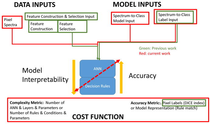
Accurate automated spectral labeling is important in the context of microspectroscopy. However, the microspectroscopy is often not only about automation and its accuracy but also about discovery and material exploratory research. Thus, the modeling objectives include accuracy and interpretability where the interpretability is understood as the semantic construct and overall complexity of the model. This paper proposes a framework for interpretable and accurate classification of microspectroscopical data as illustrated in Figure 1. More precisely, this paper demonstrates a method to derive mathematical if-then decision rules for pixel classification from Artificial Neural Networks (ANN). The proposed method combines the accuracy of ANN and the interpretability of decision rules in order bring more insight into identifying and differentiating relevant spectral patterns for various chemical components. Existing symbolic rule generation methods using ANNs extract rules from trained ANNs composed of multiple simple conditions. Usually, the input of the ANN is represented by a set of discrete numeric attributes (or features) and these methods extract if-then conditions that consist in comparing one of these features to a threshold value, similarly to Decision Trees (DT). The conditions are combined using OR, AND, or other more complex operators to form the rules (Lu et al., 1996), (Benítez et al., 1997), (Palade et al., 2001). However, as mentioned before relevant spectral features are not always easily identifiable. To address this issue, this paper presents a simple rule generation method that takes advantage of the ANN architecture to automatically extract relevant features from raw input spectral data. The hypothesis is that any spectral feature can be described as a linear combination of spectral values. At the same time, ANNs perform, in the first layer, linear transformations of the input values. Therefore, the use of ANNs is perfectly justified. Furthermore, the proposed method aims at minimizing the number of the necessary conditions per rule as well as the mathematical feature representation and, thus, yielding more compact rules that are more easily interpretable by biologists. This improvement in rule interpretability and accuracy was achieved using a combination of ANNs in tandem (series). Sequences of ANNs have been used in the past (Shaban et al., 2009), where the output of one ANN is fed to the input of another ANN. Our tandem ANN architecture is novel by generating input data for the second ANN based on extracted rules from the first ANN. It can be argued that such a minimal rule representation not only makes the rules easier to understand by human experts, but also increases the accuracy of the rules according to the minimum description length principle (Rissanen, 1983). In this sense, a quantitative evaluation of the rule accuracy is also presented.
Figure 1.
The framework of previous and current work on supervised classification modeling using ANN and Decision Rules. The bi-directional red arrow indicates the ultimate goal of accurate and interpretable classification model.
This paper is structured as follows: The following section describes the spectral rule generation method based on artificial neural networks. Section 3 presents the evaluation of this algorithm, detailing the microspectrsoscopical data, the tests performed together with the evaluation metrics. Section4 presents and discusses results based on experimental data while Section 5 gives an overall conclusion of this study.
2. Methods and materials
The first assumption of this work is that in the majority of labeling analyses experts are providing ground truth for algorithmic validation as a set of pixels with associated class labels assigned based on visual inspection of spectra. It is very rare to find a set of mathematically defined if-then rules as in the published paper by Lee et al (2013). The second assumption is that the set of if-then rules in the published paper by Lee et al (2013) is accurate and interpretable because the rules have been created by experts. The goal of our work is to discover accurate and interpretable rules automatically because the automation removes the labor of an expert doing visual mining for the if-then rules and the rule extraction is more systematic. In the majority of labeling analyses, one would start with a set of labeled pixels (first assumption) and either use decision tree machine learning model to derive a highly interpretable model or use ANN machine learning model to derive a very accurate model. This motivates our approach of designing a tandem model [ANN, rule extraction] which is novel as it aims at achieving accuracy and interpretability. While the interpretability of a tandem model is given by the resulting if-then rules, we have to validate the accuracy of the tandem model. In order to demonstrate the accuracy of the tandem model, we use the accurate and interpretable if-then rules in the published paper by Lee et al (2013) (second assumption).
In the following, the methodology of our approach and its application are described. Section 2.1 proposes a mathematical formulation of rules for spectral labeling while section 2.2 discusses the design of artificial neural networks capable of capturing such rules. Next, sections 2.3 and 2.4 describe in detail the rule generation algorithm.
2.1. Rule based model
Let x be a pixel of a spectral image, x = [x(λ1), x(λ2) … x(λn)], where x(λi) refers to the vibrational spectral value at the wavenumber λi, n is the number of spectral bands. Digital staining a spectral image consist in assigning a scalar value corresponding to a class to every pixel x in the image. A rule-based labeling model for a given pixel can be generalized as follows:
| (1) |
where Cj is a condition that has to be satisfied, NC is the number of conditions per class rule and K is the number of classes. A condition Cj should capture a spectral feature of the measured pixel. We propose the following formulation for the conditions:
| (2) |
Where wj is a vector containing real coefficients corresponding for each spectral band value and bj is a bias term. Rather than focusing on a single spectral band value, the conditions rely on features consisting of a linear combination of spectral values. We believe that such a representation can capture the possible spectral features capable of differentiating biochemical components such as the presence of single or multiple peaks, the ratio of peaks at two different bands, peak, shoulders, or spectral shifts between bands. The ≥ inequality does not limit the possibilities of condition formulation since a simple multiplication by −1 can invert the inequality condition.
2.2. ANN representation
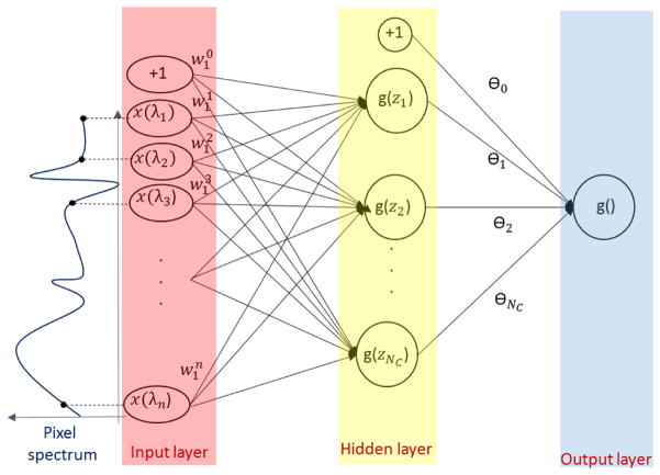
The rule formulation in the previous section can be represented in a straight-forward manner using a feed-forward artificial neural network with one hidden layer like in Figure 2. The inputs of the network are the spectral band values x. The number of the hidden nodes in the hidden layer corresponds to the overall number of conditions and the number of outputs corresponds to the number of labels or classes. For simplicity reasons, a single-output network is represented in this figure. The node activation is performed using the sigmoid function g(z) = 1/(1 + exp(−z)). The rule for a class i can be written as:
| (3) |
Figure 2.
One hidden layer ANN design for spectral pixel classification for one class (label). For the condition C1, . The number of hidden nodes corresponds to the number of conditions needed for this class.
Where and θj represent the weights of each condition. One configuration which represents exactly Eq. 1 and Eq. 2 is θj = 1 for j = 1 … Nc, θ0 = 0.5 and . Obviously, rules described by Eq. 1 using Eq. 3 can be represented using other configurations. In this subsection, we have shown how to map rules for spectral pixel classification on artificial neural networks with one hidden layer. The following subsection describes a method of retrieving rules such as those presented in Section 2.1 from a trained ANN.
2.3. Rule generation algorithm
This subsection tackles the following challenge: given a well-trained ANN with one or multiple hidden layers with one or multiple outputs, how can rules such as those described in Section 2.1 be retrieved. The method is agnostic to the input spectral data, in the sense that the number of conditions per rule or the spectral bands of interest are not previously known. The rule retrieval algorithm consists of the next steps:
2.3.1. Condition inversion weights
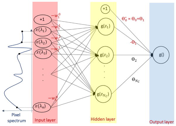
Since the desired conditions to be retrieved are in the form described by Eq. 2 (i.e spectral feature ≥ 0 ), the negative j weights need to be inverted. For this purpose, we make use of the property of the sigmoid function: g(z) = 1−g(−z). The rule described by Eq. 3 can be reformulated as follows:
| (4) |
with: and .
Figure 3 shows an example of weight inversion for the ANN depicted in Figure 2. The two neural networks are equivalent in the sense that given the same input data they produce exactly the same output.
Figure 3.
One hidden layer ANN with one inverted upper weight: θ1* = −θ1. Note that the sign change for θ1 implies a sign change for all the weights (w1) linking the input data with the first hidden node. This ANN is equivalent to the one in Figure 2
2.3.2. Condition selection
The number of conditions NC for a class rule needs to be estimated automatically by the algorithm. This task can be achieved during the network training and optimization phase by training and testing multiple configurations of ANNs and finally choosing the lowest number of hidden nodes that produce the highest accuracy. Moreover, some conditions corresponding to hidden nodes might have a low contribution to the final decision rule. This step aims at discarding these type of conditions. However, this can be a very computationally expensive task. The contribution of each condition Cj to the spectral labeling rule is directly proportional with the magnitude of the weight θj. Therefore, only conditions corresponding to hidden nodes with weights that have a high enough magnitude are considered. The rule described in Eq. 4 is modified as follows:
| (5) |
with: and .
The threshold θC represents a fraction of the maximum magnitude of the condition weights. The bias term needs to be updated for this step as well. If the first step yielded an equivalent neural network configuration as the initial one (Eq.4 ⇔ Eq.3) this step does not yield in an equivalent configuration. However, it can be easily shown that Eq. 5 ⇒ Eq. 4. This means that every spectral pixel labeled as class i using Eq. 5 will always be labeled as class i using Eq. 4 or Eq. 3.
2.3.3. Condition extraction
Eq.5 expresses the rule to assign a label i to a spectral pixel. This next step breaks the rule expressed by Eq.5 into a set of simple conditions. More precisely, it formulates a rule Ri that assigns a label i to a pixel if a set of simple conditions are satisfied: Ri − → C1 ∧ C2 ∧ … ∧ CNC. Eq.5 implies that the label i is assigned to a pixel if . Since are positive and are in the (0, 1) interval, there exists a set of minimal values Tj for each such that Eq. 5 is satisfied:
| (6) |
The values Tj can be determined by minimizing subject to and . For relatively close values, the following common threshold solution satisfies the condition in Eq. 5 . Considering the properties of the sigmoid function, each condition can be written as follows: which can be further expressed as:
| (7) |
Next a selection process such as the one similar to the one described in Step 2.3.2 is performed. By discarding the spectral band values that contribute very little to each condition, the rendering of rule conditions becomes simpler and easier to interpret. The extracted rules are more restrictive than the artificial neural networks, in the sense that a pixel that is labeled as class i will always be labeled as class i ∈ [1,K] using the ANN but not necessarily vice-versa.
2.4. Rule refinement strategy
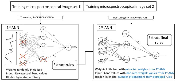
The rule generation algorithm presented in the previous section discards a number of low value weights thus approximating the conditions. For this reason, we propose a rule refinement method which applies an additional simpler ANN to the rule generation process. Figure 4 summarizes this idea.
Figure 4.
Rule refinement using two ANNs in tandem. The extracted rules from the 1st ANN are used to initialize the weight of the second one
A first set of rules (together with the modified ANNs weights) is retrieved using the process described in the previous subsection. A second ANN is built in the following manner: instead of having as an input all the spectral band values, only the band values associated with non-zero weights from the initial processed ANN are considered. The weights of this second ANN are initialized with the non-zero weights from the initial ANN.
3. Experimental set-up
The evaluation of the rule generation method is performed against a reference rule-based model for assigning four labels (Nucleus, Cytosol, Lipid, and Mineral) published in Lee et al. (2013). For more details on the experimental setup and the image acquisition one may refer to Lee et al. (2013).
3.1. Data set
The data set is composed of 60 broadband coherent anti-Stokes Raman scattering (BCARS) cellular images consisting of 100×100 pixels. Each image pixel contains 560 spectral points from 500 cm−1 to 3400 cm−1. The spectral resolution is approximately 5 cm−1. Decision making of each chemical label is based on the second derivative of a BCARS spectrum at each image pixel. The reference rule-based labeling of pixels is summarized below for the four classes:
-
Cytosol :
x(2845cm−1 to 2856cm−1) − x(2877cm−1 to 2886cm−1) > −3
x(2935cm−1 to 2942cm−1) > 10
x(2933cm−1 to 2942cm−1) − x(2854cm−1 to 2863cm−1) > 0
-
Nucleus
x(2877cm−1 to 2886cm−1) − x(2854cm−1 to 2856cm−1) > 2
x(2935cm−1 to 2942cm−1) − x(2965cm−1 to 2966cm−1) > 18
x(975cm−1 to 985cm−1) − x(953cm−1 to 965cm−1) > −3
-
Lipids
x(2854cm−1 to 2863cm−1) − x(2933cm−1 to 2942cm−1) > 11
-
Minerals
x(953cm−1 to 965cm−1) − x(975cm−1 to 985cm−1) > 10
-
Background
Otherwise
x(λ1 to λ2) refers to the average amplitude of the spectra between λ1 and λ2. For this data set, the four classes are not equally represented: 29 % of the pixels are cytosol, 7 % nuclei, 1.5 % lipids and only 0.15 % minerals. The rest is background.
3.2. Tests performed
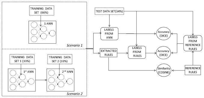
The following two scenarios were considered: first, images were labeled using only one ANN and a first set of rules were extracted using the method described in section 2.3 (no refinement). The second scenario consisted in using the rule refinement strategy described in section 2.4. Figure 5 depicts the evaluation tests. For each class of materials we performed a binary classification using ANN (One class versus all). The number of hidden nodes in the hidden layer was varied from 2 to 6, 4 yielding the best performance. The threshold θC was set to in equation 5, meaning that neurons associated with weights less than 0.2 times the maximum weight value in one layer will be discarded in the rule generation process. Both the classifiers accuracy and the extracted rule accuracy were measured against the reference rule-based model labels. In addition, the similarities between the extracted rules and the reference rules were computed. The next subsection describes the metrics used.
Figure 5.
Experimental setup for evaluation using two ANN-based classifiers. The training data set is divided into two subsets which are used to train the two ANNs. The labels output using the ANN classifier as well as the labels output using the extracted rules are compared against the labels output using the reference rules
3.3. Evaluation metrics
The digital labeling outputs of the ANN-based methods were compared against the labels from the reference rule-based model using the DICE index (Dice, 1945):
| (8) |
where Di represents the DICE similarity index for the class i, represent the set of pixels labeled as class i using the reference rule-based model and represent the set of pixels labeled as class i using one supervised method. The DICE index ranges from 0 (no overlap between the segmentations) to 1 (identical segmentations). A DICE index equal or above 0.7 denotes a good agreement between the two segmentations. Moreover, we were not interested only in the accuracy of the labeling but also in the accuracy of the extracted rules. For this purpose, the following metric was used to compare two conditions accuracy of the extracted rules. For this purpose, the following metric was used to compare two conditions and :
| (9) |
represents the absolute value of the cosine of the angle between the two vectors in the spectral hyperspace representing the conditions such as described in section 2.1.
4. Results
This section presents the evaluation results of the experiment described in Section 3. More precisely, rules extracted from one single ANN are compared with rules extracted from a tandem of ANNs. Both labeling accuracy and rule similarity are computed for evaluation.
4.1. Labeling accuracy
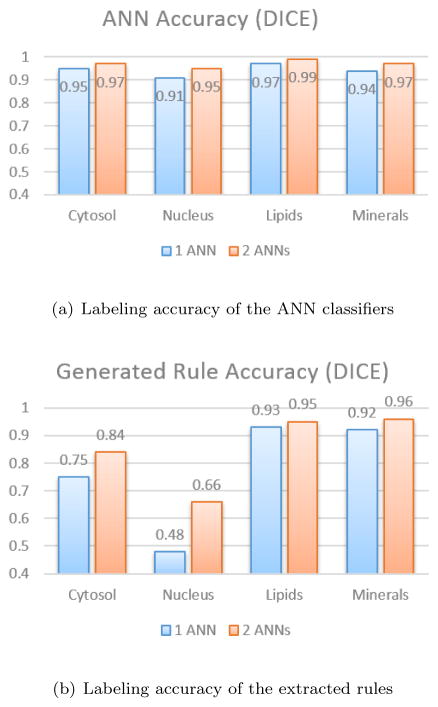
Figure 6(a) shows the accuracy of the labeling for each class of materials (cytosol, nucleus lipids and minerals) in terms of the dice index. Using two ANNs in tandem improves the overall accuracy of the classifier from 2 % up to 4 % of the maximum accuracy. Figure 6(b) shows the accuracy of the labeling for each class in terms of the dice index in both case scenarios: where rules are generated using only one trained ANN and where rules are generated using two ANNs in tandem. As expected, the rules generated using two ANNs are more accurate (from 2 % up to 18 % of the maximum accuracy).
Figure 6.
Labeling accuracy in terms of dice index for the two evaluation scenarios (1 ANN versus 2 ANNs)
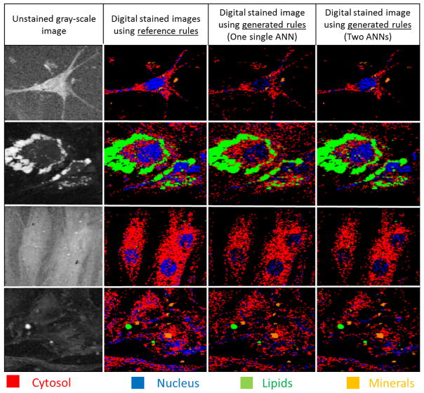
It can be noted that, overall, the generated rules are less accurate than the ANN classifier (from 1 % up to 43 % of the maximum accuracy). Figure 7 shows four examples of pseudo-labeled BCARS images. The unstained gray-scale images are constructed with the square root of total raw spectrum (first row of Figure 7). The labeled images on the second row are obtained using the reference rules while the images on the third and fourth rows are created using the extracted rules from the classifiers based on one ANN and two ANNs respectively. The visual inspection of this image confirms the aforementioned numerical observations i.e., the generated rules seem to correctly identify lipids (green), minerals (orange) and most of the cytosol pixels (red) with respect to the reference model whereas a part of nucleus pixels (blue) are mistaken with background pixels (black).
Figure 7.
Pseudo-labeled BCARS images using the reference and extracted rules
4.2. Rule similarity
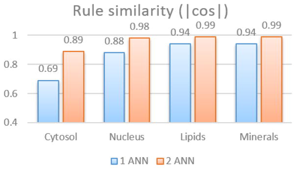
Figure 8 presents the rule similarity between the extracted rules from the ANN classifiers and the reference rules used for labeling. The rule similarity is computed using Equation 9. The rule similarity values are in agreement with the dice indices except for the nucleus case, where although the rule similarity is high, the dice index remains low. For a more detailed comparison one may refer to the Appendix of this document.
Figure 8.
Rule similarity in terms of cosine between the vectors describing the rules (1 ANN versus 2 ANNs).
4.3. Complexity analysis
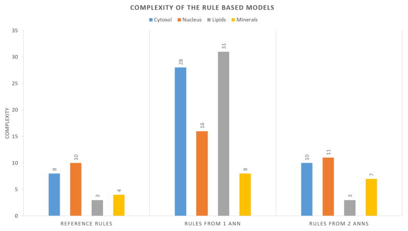
Figure 9 illustrates the complexity of the rule-based models derived from one ANN and two ANNs, and compared against the complexity of the reference rules. The complexity was computed as the overall sum of the number of bands per condition. It can be observed that the rules extracted from two ANNs in tandem are less complex compared to the rules extracted using only one ANN. The complexity of one or two ANNs was also measured and found to be on average two orders of magnitude larger than the complexity of the if-then rules.
Figure 9.
Complexity of the decision making process for the different classifying methods. The complexity is proportional to the number of input bands needed to make the decision.
5. Discussion
This paper demonstrated a novel method that automatically constructs and selects discriminatory features from raw spectral bands using ANNs (i.e., feature engineering has been eliminated). These features are used to form interpretable if-then decision rules for microspectroscopic pixel classification. The tests show given training pixel labels one can derive interpretable if-then rule model with an accuracy ranging from 66 % to 96 %. Moreover, our tests show that the extracted rule similarity with reference rules ranges from 69 %–99 % using the cosine metric. The novel strategy of using two ANNs in tandem for rule generation improves not only the accuracy of the rules but also reduces the complexity of these rules thus making them more interpretable by human experts.
By removing the spectral bands associated with low magnitude weights in the first ANN, the number of input spectral values for the second ANN was reduced. The same reduction was applied during rule extraction from the second ANN and therefore the resulting rule-based model is much simpler than the one derived from one ANN (see Figure 9).
The technique described in this paper could also be compared to other existing rule-generation methods such as decision trees or random forests. However, the results of existing rule-generation methods would have to be pruned based on some cost function to a level such that the decision rules can be easily interpreted by humans (low level of complexity). In addition, the resulting rules would not consist of spectral band differences but only spectral bands which would deviate significantly from ground truth rules. It is conceivable to add a decision tree as a third layer to the overall classifier. In this case, the ANNs would be responsible for feature construction and feature selection while the decision tree would build the final if-then rules.
From an application point of view, the method presented in this paper can bring more insight into identifying relevant spectral patterns of various chemical components for pixel classification in microspectroscopy. Reference rule-based models such as the one used for evaluation are rarely reported since the majority of experts annotate pixel spectra by visual inspection without providing any if-then rules. Annotating individual pixels yields a small number of training samples in comparison to the large number of training samples obtained from if-then rule-based annotation. Ideally for validation, one would need a large number of training data obtained by independent manual pixel labeling and if-then rule discovery. In our case, the expert discovered the if-then rules by visually inspecting a large number of pixel spectra. Therefore, our validation is as reliable as possible given the experimental discovery setup. The method described in this paper can be applied to discover new interpretable mathematical rules from annotated data based on visual inspection for other materials than the ones presented in this paper.
Acknowledgments
This research did not receive any specific grant from funding agencies in the public, commercial, or not-for-profit sectors.
Appendix: extracted rules
| Classifier accuracy (Dice) | Extracted rule CYTOSOL | Rule accuracy (Dice) | Rule similarity | ||
|---|---|---|---|---|---|
| Reference rule model | C1 | 0.5·x(2849.1) + 0.5 ·x (2855.02) − 0.5 ·x(2878.9) − 0.5 ·x (2884.9) > −3 | |||
| C2 | −0.5 ·x (2855.0) −0.5 ·x (2861.0) + 1·x (2938.8)>0 | ||||
| C3 | 1.00 ·x (2938) > 10 | ||||
| One ANN | 0.95 | C1 | + (0.98) ·x(2849.07) + (0.91) ·x(2855.02) + (−0.90) ·x(2878.87) + (−1.01) ·x(2884.85)>−3.06 | 0.75 | 0.69 |
| C2 | + (0.14) ·x(918.45)+ (−0.16)·x(986.37)+ (0.12) ·x(1078.04)+ (0.13)·x(1138.32)+ (−0.14) ·x(1327.33)+ (−0.13) ·x(1453.12)+ (0.13)·x(1596.26)+ (−0.14)·x(2404.75)+ (−0.17)·x(2843.13)+ (0.15) ·x(2849.07)+ (0.41) ·x(2855.02) + (0.20) ·x(2860.98)+ (0.22) ·x(2938.83)+ (0.15) ·x(3035.78)+ (−0.13) ·x(3146.36)+ (−0.13) ·x(3189.80)>1.82 | ||||
| C3 | + (−0.20) · x(2855.02) + (0.44) · x(2938.83) + (−0.15) ·x(2975.04) + (−0.20) ·x(3011.43) + (−0.14) ·x(3023.59) + (−0.14) ·x(3047.99) + (−0.18) ·x(3398.00)> 5.79 | ||||
| C4 | + (1.20) ·x(2938.83)>3.66 | ||||
| Double ANN | 0.97 | C1 | + (4.34) · x(2849.07) + (7.55) · x(2855.02) + (−5.99) ·x(2878.87) + (−5.92) ·x(2884.85)>−11.34 | 0.84 | 0.89 |
| C2 | + (−3.08) ·x(2855.02) + (−8.85) ·x(2860.98) + (3.59) ·x(2932.82) + (5.75) ·x(2938.83) + (5.59) ·x(2944.86)> 1.31 | ||||
| C3 | + (3.39) ·x(2938.83)>32.95 | ||||
| Classifier accuracy (Dice) | Extracted rule NUCLEUS | Rule accuracy (Dice) | Rule similarity | ||
|---|---|---|---|---|---|
| Reference rule model | C1 | −1 ·x(2855) + 0.5 ·x(2878.9) + 0.5 ·x(2884.8) > 2 | |||
| C2 | +1·x(2938.8)−1.s2969 > 18 | ||||
| C3 | (−0.33).s(954.6) − (0.33).s(959.1) −0.33.s(963) + 0.5.s(977.3) + 0.5.s(981) > −3 | ||||
| One ANN | 0.91 | C1 | + (−0.82) ·x(2849.07) + (−2.02) ·x(2855.02) + (−0.79) ·x(2860.98) + (1.36) ·x(2878.87) + (1.30) ·x(2884.85)>6.21 | 0.48 | 0.88 |
| C2 | + (0.19) ·x(2932.82)+ (0.55) ·x(2938.83)+ (0.18) ·x(2944.86)+ (−0.31) ·x(2962.95)+ (−0.19) ·x(2968.99)> 11.09 | ||||
| C3 | + (−0.80) ·x(954.59) + (−0.93) ·x(959.12) + (−0.78) ·x(963.65) + (0.45) ·x(972.73) + (1.27) ·x(977.27) + (1.27) ·x(981.82)> 2.02 | ||||
| Double ANN | 0.95 | C1 | + (−2.66) ·x(2855.02) + (1.56) ·x(2878.87) + (1.32) ·x(2884.85)>9.34 | 0.66 | 0.98 |
| C2 | + (1.14) ·x(2938.83) + (−0.61) ·x(2962.95) + (−0.54) ·x(2968.99)> 23.52 | ||||
| C3 | + (−0.67) ·x(954.59) + (−0.76) ·x(959.12) + (−0.74) ·x(963.65) + (1.03) ·x(977.27) + (1.14) ·x(981.82)>−3.98 | ||||
| Classifier accuracy (Dice) | Extracted rule LIPIDS | Rule accuracy (Dice) | Rule similarity | ||
|---|---|---|---|---|---|
| Reference rule model | C1 | + (0.5) ·x(2855.02) + (0.5) ·x(2860.98) + (−1) ·x(2938.83)> 11 | |||
| One ANN | 0.97 | C1 | + (0.25) ·x(2855.02) + (0.26) ·x(2860.98) + (−0.17) ·x(2932.82) + (−0.34) ·x(2938.83) + (−0.22) ·x(2944.86) + (−0.10) ·x(3220.98) + (−0.11) ·x(3239.75) + (0.24) ·x(3398.00)>3.42 | 0.93 | 0.94 |
| C2 | + (0.27) ·x(2855.02)+ (0.26) ·x(2860.98)+ (−0.18) ·x(2932.82)+ (−0.32) ·x(2938.83)+ (−0.18) ·x(2944.86)+ (0.10) ·x(3072.46)+ (−0.10) ·x(3196.03)+ (−0.12) ·x(3220.98)+ (−0.13) ·x(3239.75)+ (−0.10) ·x(3264.85)+ (0.13) ·x(3398.00)>3.57 | ||||
| C3 | + (0.23) ·x(2855.02) + (0.26) ·x(2860.98) + (−0.16) ·x(2932.82) + (−0.32) ·x(2938.83) + (−0.19) ·x(2944.86) + (−0.10) ·x(3208.49) + (−0.11) ·x(3214.74) + (−0.12) ·x(3220.98) + (−0.10) ·x(3227.23) + (−0.10) ·x(3233.49) + (−0.11) ·x(3239.75) + (0.12) ·x(3398.00)> 3.86 | ||||
| Double ANN | 0.99 | C1 | + (0.33) ·x(2855.02) + (0.34) ·x(2860.98) + (−0.46) ·x(2938.83)>7.60 | 0.95 | 0.99 |
| C2 | + (0.33) ·x(2855.02) + (0.34) ·x(2860.98) + (−0.46) ·x(2938.83)>7.60 | ||||
| C3 | + (0.33) ·x(2855.02) + (0.34) ·x(2860.98) + (−0.46) ·x(2938.83)>7.60 | ||||
| Classifier accuracy (Dice) | Extracted rule MINERALS | Rule accuracy (Dice) | Rule similarity | ||
|---|---|---|---|---|---|
| Reference rule model | C1 | 0.33·x(954.59) + 0.33·x(959.12) + 0.33.s(963.65) − 0.5.s(977.27) − 0.5.s(981.82) > 10 | |||
| One ANN | 0.94 | C1 | + (0.12) ·x(950.06)+ (0.26) ·x(954.59)+ (0.34) ·x(959.12)+ (0.28) ·x(963.65)+ (0.11) ·x(968.19)+ (−0.21) ·x(977.27) + (−0.22) ·x(981.82)+ (−0.13) ·x(986.37)>9.65 | 0.92 | 0.94 |
| C2 | + (0.12) ·x(950.06)+ (0.27) ·x(954.59)+ (0.34) ·x(959.12)+ (0.29) ·x(963.65)+ (0.12) ·x(968.19)+ (−0.21) ·x(977.27)+ (−0.22) ·x(981.82)+ (−0.14) ·x(986.37)>9.99 | ||||
| C3 | + (0.12) ·x(950.06)+ (0.26) ·x(954.59) + (0.34) ·x(959.12) + (0.28) ·x(963.65) + (0.12) ·x(968.19) + (−0.20) ·x(977.27)+ (−0.22) ·x(981.82)+ (−0.14) ·x(986.37)> 10.05 | ||||
| Double ANN | 0.97 | C1 | + (0.18) ·x(950.06) + (0.32) ·x(954.59) + (0.36) ·x(959.12) + (0.28) ·x(963.65) + (−0.20) ·x(977.27) + (−0.20) ·x(981.82) + (−0.13) ·x(986.37)> 9.65 | 0.96 | 0.99 |
| C2 | + (0.18) ·x(950.06) + (0.32) ·x(954.59) + (0.36) ·x(959.12) + (0.28) ·x(963.65) + (−0.20) ·x(977.27) + (−0.20) ·x(981.82) + (−0.13) ·x(986.37)> 9.65 | ||||
Footnotes
Disclaimer
Commercial products are identified in this document in order to specify the experimental procedure adequately. Such identification is not intended to imply recommendation or endorsement by NIST, nor is it intended to imply that the products identified are necessarily the best available for the purpose.
References
- Baker MJ, Trevisan J, Bassan P, Bhargava R, Butler HJ, Dorling KM, Fielden PR, Fogarty SW, Fullwood NJ, Heys KA, et al. Using fourier transform ir spectroscopy to analyze biological materials. Nature protocols. 2014;9(8):1771–1791. doi: 10.1038/nprot.2014.110. [DOI] [PMC free article] [PubMed] [Google Scholar]
- Benítez JM, Castro JL, Requena I. Are artificial neural networks black boxes? Neural Networks, IEEE Transactions on. 1997;8(5):1156–1164. doi: 10.1109/72.623216. [DOI] [PubMed] [Google Scholar]
- Bhargava R. Infrared spectroscopic imaging: the next generation. Applied spectroscopy. 2012;66(10):1091–1120. doi: 10.1366/12-06801. [DOI] [PMC free article] [PubMed] [Google Scholar]
- Dice LR. Measures of the amount of ecologic association between species. Ecology. 1945;26(3):297–302. [Google Scholar]
- Dochow S, Bergner N, Krafft C, Clement J, Mazilu M, Praveen BB, Ashok PC, Marchington R, Dholakia K, Popp J. Classification of raman spectra of single cells with autofluorescence suppression by wavelength modulated excitation. Analytical Methods. 2013;5(18):4608–4614. [Google Scholar]
- Ellis DI, Goodacre R. Metabolic fingerprinting in disease diagnosis: biomedical applications of infrared and raman spectroscopy. Analyst. 2006;131(8):875–885. doi: 10.1039/b602376m. [DOI] [PubMed] [Google Scholar]
- Kee TW, Cicerone MT. Simple approach to one-laser, broadband coherent anti-stokes raman scattering microscopy. Optics letters. 2004;29(23):2701–2703. doi: 10.1364/ol.29.002701. [DOI] [PMC free article] [PubMed] [Google Scholar]
- Lasch P, Diem M, Hänsch W, Naumann D. Artificial neural networks as supervised techniques for ft-ir microspectroscopic imaging. Journal of chemometrics. 2006;20(5):209–220. doi: 10.1002/cem.993. [DOI] [PMC free article] [PubMed] [Google Scholar]
- Lee YJ, Vega SL, Patel PJ, Aamer KA, Moghe PV, Cicerone MT. Quantitative, label-free characterization of stem cell differentiation at the single-cell level by broadband coherent anti-stokes raman scattering microscopy. Tissue Engineering Part C: Methods. 2013;20(7):562–569. doi: 10.1089/ten.tec.2013.0472. [DOI] [PMC free article] [PubMed] [Google Scholar]
- Levin IW, Bhargava R. Fourier transform infrared vibrational spectroscopic imaging: Integrating microscopy and molecular recognition*. Annu Rev Phys Chem. 2005;56:429–474. doi: 10.1146/annurev.physchem.56.092503.141205. [DOI] [PubMed] [Google Scholar]
- Lu H, Setiono R, Liu H. Effective data mining using neural networks. Knowledge and Data Engineering, IEEE Transactions on. 1996;8(6):957–961. [Google Scholar]
- Mayerich D, Walsh MJ, Kadjacsy-Balla A, Ray PS, Hewitt SM, Bhargava R. Stain-less staining for computed histopathology. Technology. 2015;3(01):27–31. doi: 10.1142/S2339547815200010. [DOI] [PMC free article] [PubMed] [Google Scholar]
- Miljković M, Chernenko T, Romeo MJ, Bird B, Matthäus C, Diem M. Label-free imaging of human cells: algorithms for image reconstruction of raman hyperspectral datasets. Analyst. 2010;135(8):2002–2013. doi: 10.1039/c0an00042f. [DOI] [PubMed] [Google Scholar]
- Ong YH, Lim M, Liu Q. Comparison of principal component analysis and biochemical component analysis in raman spectroscopy for the discrimination of apoptosis and necrosis in k562 leukemia cells. Optics express. 2012;20(20):22158–22171. doi: 10.1364/OE.20.022158. [DOI] [PubMed] [Google Scholar]
- Palade V, Neagu D-C, Patton RJ. Computational Intelligence. Theory and Applications. Springer; 2001. Interpretation of trained neural networks by rule extraction; pp. 152–161. [Google Scholar]
- Rissanen J. A universal prior for integers and estimation by minimum description length. The Annals of statistics. 1983:416–431.
- Shaban K, El-Hag A, Matveev A. A cascade of artificial neural networks to predict transformers oil parameters. IEEE Transactions on Dielectrics and Electrical Insulation. 2009;16(2):516–523. [Google Scholar]
- Tiwari S, Bhargava R. Extracting knowledge from chemical imaging data using computational algorithms for digital cancer diagnosis. The Yale journal of biology and medicine. 2015;88(2):131–143. [PMC free article] [PubMed] [Google Scholar]


