Validation of surface-to-volume ratio measurements derived from oscillating gradient spin echo on a clinical scanner using anisotropic fiber phantoms

Abstract

The short-time surface-to-volume ratio (S/V) limit [Mitra et al., Phys. Rev. Lett. 68, 3555 (1992)] can disentangle the free diffusion coefficient from geometric restrictions to diffusion. Biophysical parameters, such as the S/V of tissue membranes, can be used to interpret microscopic length scales non-invasively. However, due to gradient strength limitations on clinical MRI scanners, Pulsed Gradient Spin Echo (PGSE) measurements are impractical for probing the S/V limit. To achieve this limit on clinical systems, an Oscillating Gradient Spin Echo (OGSE) sequence was developed. Two phantoms containing 10 fiber bundles, each consisting of impermeable aligned fibers with different packing densities, were constructed to achieve a range of S/V values. The frequency-dependent diffusion coefficient, D(ω), was measured in each fiber bundle using OGSE with different gradient waveforms (cosine, stretched cosine, and trapezoidal), while D(t) was measured from PGSE and stimulated-echo measurements. The S/V values derived from the universal high-frequency behavior of D(ω) were compared against those derived from quantitative proton density measurements using single spin echo (SE) with varying echo times, and from magnetic resonance fingerprinting (MRF). S/V estimates derived from different OGSE waveforms were similar and demonstrated excellent correlation with both SE- and MRF-derived S/V measures ( $\rho \ge 0.99$). Furthermore, there was a smoother transition between OGSE frequency f and PGSE diffusion time when using $t_{\mathrm{eff}}^{(S/V)}=9/(64f)$, rather than the commonly used $t_{\mathrm{eff}}=1/(4f)$, validating the specific frequency/diffusion time conversion for this regime. Our well-characterized fiber phantom can be used for the calibration of OGSE and diffusion modeling techniques, as the S/V ratio can be measured independently using other MR modalities. Moreover, our calibration experiment offers an exciting perspective of mapping tissue S/V on clinical systems.

Short Abstract

We created an anisotropic fiber phantom that has 4 fiber bundles of various packing densities, which manifest into differences in surface-to-volume (S/V). Due to the simple bundle geometry, S/V from diffusion could be confirmed through an independent measurement from proton density (PD). Using oscillating gradient spin echo (OGSE), we acquired within the short-time S/V-limit to derive S/V and compared with S/V derived from quantitative PD, which we obtained from single Spin Echo and Magnetic Resonance Fingerprinting.

Introduction

The apparent diffusion coefficient (ADC), obtained from diffusion weighted MRI (1,2), is a highly sensitive but non-specific biomarker of tissue complexity. ADC derives its contrast mostly from microscopic tissue features, which may include cell size, cellularity, and membrane permeability. Moreover, ADC contrast could also arise from varying intrinsic diffusion coefficients, i.e. in the intra- and extracellular space or in glandular fluid. Since most pathologies occur on the cellular level, this biomarker has gained widespread usage in the clinic, particularly in stroke detection (3) and cancer screening (4).

The specificity of ADC to tissue microstructure can be unlocked through biophysical modeling. Particularly, varying the diffusion time t allows for probing relevant biophysical length scales. Biophysical modeling and measurement of D(t) was first performed in the pioneering 1979 work of Tanner (5). There, he measured water diffusion coefficient in frog muscle by combining pulsed gradient spin echo (PGSE), stimulated-echo (STEAM), and oscillating gradient spin echo (OGSE) sequences to study the range of t from 0.3 ms to 2.4 s, spanning almost 4 orders of magnitude, and estimated membrane parameters from his exact solution of diffusion restricted by periodic membranes in one dimension. Further studies revealed that, generally speaking, an observed time-dependence in D(t) is a signature of non-Gaussian diffusion (6). Using biophysical modeling, given D(t), it is possible to extract the relevant length scale over which diffusion is either hindered or restricted (6–10). This observation has potentially important clinical implications, as D(t) could provide micrometer-level biomarkers of tissue integrity and function at the scale far below the attainable MRI resolution.

Despite its potential, research on D(t) did not find its way into the imaging community until the turn of the century (11,12). During the 1990s, there was a strong interest in D(t), both theoretical and experimental, focused on porous media studies using NMR for materials characterization. In particular, this interest in time-dependent diffusion stems from the realization that in the short-time limit the behavior of D(t) in a statistically isotropic medium becomes universal (13),

$$D(t)\simeq D_0\left(1-\frac{4}{3d\sqrt{\pi }}\frac{S}{V}\sqrt{D_{0}t}\right),$$ [1]

depending only on the surface-to-volume ratio S/V of the restrictions, and on the unrestricted (free) diffusivity D₀, where d is the spatial dimension. As the fraction of walkers exposed to the surfaces increases, the walkers become more sensitive to geometrical features and permeability, which escalates the model’s complexity and adds higher orders of t to equation [1]. From an experimental perspective, acquiring D(t) within the S/V limit $\frac{S}{V}\sqrt{D_{0}t}\ll 1$ allows for a straightforward determination of S/V (14).

Early NMR applications used the above limit [1] to quantify S/V within porous media (15,16) as well as biological tissues (17). All of these experiments were performed using a PGSE sequence, which defines the diffusion time, Δ, as the spacing between the front lobes of the dephasing and rephrasing (constant) gradient pulses. Nowadays PGSE forms the basis of practically every clinical diffusion measurement. The diffusion weighting for PGSE is

$$b={\gamma }^2{G}^2{\delta }^2\left(\Delta -\frac{\delta }{3}\right),$$ [2]

where γ is the gyromagnetic ratio, δ is the width of the gradient pulse, and G is the diffusion gradient strength. In practice, short Δ and δ will result in negligible b, unless G is increased dramatically. Hence, given the relatively weak gradients available on clinical scanners, the PGSE approach is unable to probe the S/V limit for the vast majority of tissue structures.

A promising alternative is switching to OGSE (5,18,19), which replaces the two rectangular diffusion pulses with oscillating gradients. OGSE alleviates the high G requirement by accumulating diffusion weighting over each period of oscillation, N, such that the resulting diffusion weighting

$$b=\frac{{\gamma }^2{G}^2}{2{\omega }^2}·T,T=N\mathrm{\tau }$$ [3]

scales with N, or equivalently, with the total OGSE waveform duration T, where period of oscillation τ = 2π/ω. This decouples the diffusion time, which is of the order of τ (as described in more detail below), from the overall waveform duration T.

The corresponding analytic form of the S/V limit in the frequency domain was recently derived (20):

$$D\left(\omega \right)\equiv \mathrm{Re}\mathcal{D}\left(\omega \right)\simeq D_0\left(1-\frac{1}{d\sqrt{2}}\frac{S}{V}\sqrt{\frac{D_0}{\omega }}\right),N\gg 1.$$ [4]

Equations [1] and [4] describe the two equivalent ways in which the effect of restrictions to diffusion enter into the different diffusion measurement schemes, PGSE and OGSE. These relations show that the PGSE and OGSE in the short-time / high frequency limit carry the same information content about tissue geometry.

In general, converting between D(t) and D(ω) is non-trivial because of the non-local relation between these two metrics (6), akin to a Fourier transform. This makes the OGSE/PGSE conversion dependent on the physics of diffusion – i.e. on the functional form of the time-dependent diffusion coefficient. This non-local character of the time-frequency relation has been largely ignored so far, and instead the empirical identification of “effective OGSE diffusion time” (21–25)

$$t_{\mathrm{eff}}=\frac{1}{4f},f=\frac{1}{\tau }=\frac{\omega }{2\pi },$$ [5]

has been overwhelmingly used, irrespective of the diffusion regime or a type of medium/tissue. The above short-time limits [1] and [4] already show that such identification does not generally apply. Indeed, comparing the two equivalent diffusivities [1] and [4] yields a notably different conversion

$$t_{\mathrm{eff}}^{(S/V)}=\frac{9}{64f}=\frac{9}{16}{t}_{\mathrm{eff}}.$$ [6]

Recently, OGSE has gained traction as an alterative to standard PGSE diffusion imaging techniques, leading to several in vivo studies for tissue characterization (22,23,25). For example, the S/V limit was recently demonstrated in a mouse glioma model (25). These initial results suggest that S/V is a geometric marker of tumor microstructure. However, the feasibility of the S/V limit in a clinical setting has not been evaluated yet.

In this work, we make the first necessary steps for the clinical translation of OGSE in the S/V limit. We validate the S/V quantification using D(ω) measured with an in-house developed OGSE sequence in 10 fiber bundles with a range of known S/V values, and demonstrate the first instance of achieving the S/V limit on a clinical MR scanner. Our results also corroborate the correspondence [6] between OGSE frequency and diffusion time in the short-time limit.

Methods

Fiber phantom

Two cylindrical phantoms containing respectively six and four bundles of Dyneema^® fibers (diameter $2r=17\mu \mathrm{m}$) immersed in water were constructed, according to the details provided in Ref. (26,27). Dyneema^® fibers (Dyneema^® SK75 1760 dTex, DSM) are made from ultra high molecular weight polyethylene. The monofilament fiber is chemically inert to water, is hydrophobic and impermeable to water, such that all water diffusion in the phantom will be the result of water molecules diffusing in-between fibers rather than inside them. Fiber bundles were constructed by carefully winding a Dyneema thread (containing hundreds or thousands of fibers) around two fixed rods, so that fibers are parallel to one another. Fibers were wound with 20, 30, 40, 50, 60, 70 turns (Phantom 1) in the larger phantom and 50, 75, 100, 110 turns (Phantom 2) in the smaller phantom. After winding each fiber bundle was removed from the fixed rods, inserted into a polyolefin low-temperature shrinking tube (Verasafit, Tyco Electronics), and submerged in water. All of the following steps were performed with the bundles submerged under water, to minimize susceptibility artifacts caused by air bubbles. The materials were then heated in order to shrink the tube, resulting in a uniform densely packed fiber bundle. Following shrinkage, each bundle was agitated and squeezed to remove any remaining bubbles.

Since the fiber bundles were not packed very densely, the shrinking tubes shrunk uniformly to a given diameter after heating. As a result of the different number of filaments in each, the fiber bundles differ in fiber density, which manifests into different values for the water volume fraction ϕ, and fiber S/V. When imaging, the phantom was positioned so that the fibers were aligned parallel to the magnetic field to avoid local field distributions (26–28).

Diffusion measurements

Measurements were performed on a MAGNETOM 3T PRISMA (80 mT/m) system (Siemens AG, Erlangen, Germany) with a standard 20-channel head coil.

For this project, we used an in-house developed OGSE sequence. OGSE was performed using three different gradient waveforms: trapezoidal (29,30), cosine (21) and stretched cosine gradient (31) with stretch factor 2. Non-cosine gradient waveforms were implemented for increased b-value, while suppressing zero-frequency lobes [Fig.1]. Since all of these waveforms represent cosine trains, we carefully considered the ramps needed to reach the maximal gradient amplitude at the beginning and end of the oscillating gradients. Ramps from Parsons et al. (21) and Kiselev et al. (32) were both implemented, though we preferred the ramps suggested by Parsons et al. due to the lower slew rate requirements. However, it should be noted that the ramp determination method described by Kiselev et al. results in fewer imperfections within the gradient modulation power spectra ${\left|F(f)\right|}^2$, though less practical on current clinical systems and better suited for animal scanners with high performance gradients. The elements of the b-matrix were calculated exactly in the standard way by double integrating over the gradient waveforms (33), thereby accounting for non-diffusion gradients after incorporating the imaging and spoiler gradients. All acquired trapezoidal [Fig.2(A)] and stretched cosine gradient images were performed with $b=160s/m{m}^2$, whereas cosine images were acquired with $b=120s/m{m}^2$ due to the shorter maximum duty cycle possible for the same range of frequencies. We neglect ADC corrections due to a finite number N of oscillations (34) as our N ranges between 4 and 44 (counted as the total number, i.e. before + after the refocusing pulse); we specifically maximized N for each OGSE frequency.

Figure 1.

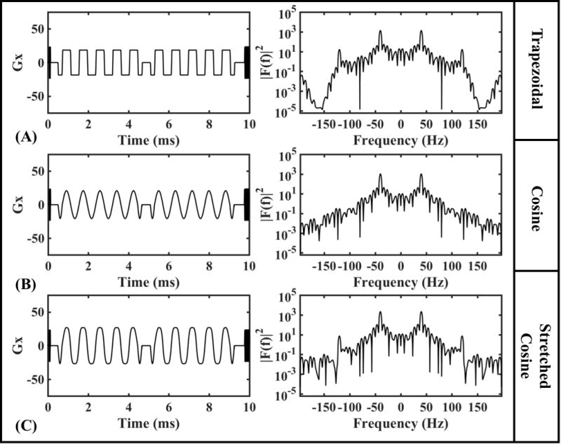
OGSE diffusion gradient waveform for 40 Hz with 10 periods and EPI train during one TR and the corresponding gradient modulation power spectra, |F(f)|², for (A) trapezoid, (B) cosine, and (C) stretched cosine gradients.

Figure 2.

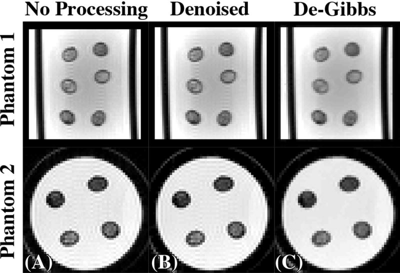
Demonstration of the post-processing steps on an EPI b = 0-image (A) from phantom 1 (top) and phantom 2 (bottom) derived from the trapezoidal gradient waveform first denoising using Marchenko-Pastur Principle Component Analysis (B) followed by Gibbs Ringing correction via local subvoxel shifts (C).

Pulsed gradient diffusion acquisitions using monopolar pulsed gradient spin echo (PGSE) and stimulated echo acquisition mode (STEAM) (WIP511E) were also acquired to examine diffusion behavior at long t in comparison to OGSE [Fig.3(A,B)] with 2 shells with b-values of 160 and 500 $s/m{m}^2$ for phantom 1 and 160 and 750 $s/m{m}^2$ for phantom 2. An additional higher b shell was included to counteract the contribution of imaging gradients to diffusion weighting (35) which become greater at longer diffusion times. Measurement parameters for the acquisition of diffusion-weighted images are summarized in Table 1. D(t) derived from OGSE and PGSE (Monopolar, STEAM) sequences was compared with t_eff based on equations [5] and [6].

Figure 3.

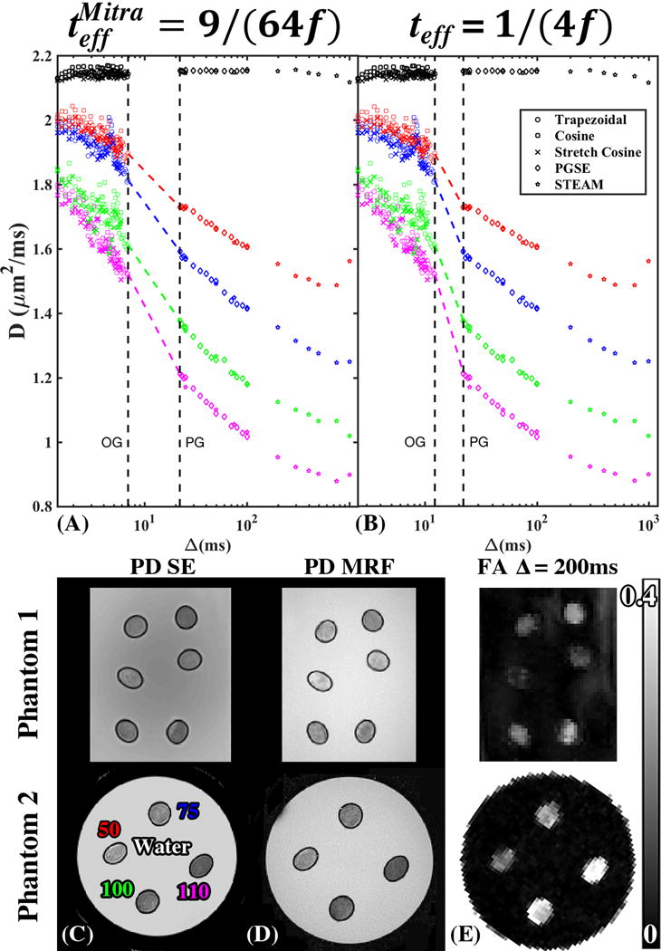
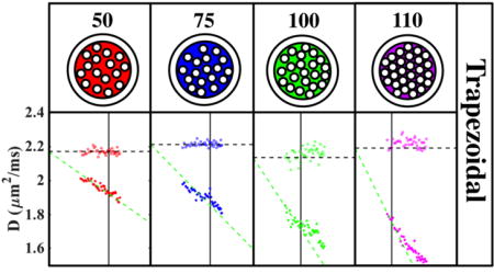
Time dependence of the diffusivity D in the 4 fiber bundles of Phantom 2 measured using different OGSE waveforms with f converted to time, t, according to (A) t_eff = 1/(4f) and (B) $t_{\mathrm{eff}}^{(S/V)}=9/(64f)$, as well as using PGSE and STEAM measurements from Phantom 2. The black points represent the mean diffusivity of surrounding water. The colored dots are the radial diffusivities within the fiber bundles. The colored dashed lines connect OGSE and PGSE. Axial cross section of both fiber phantoms showing (C) SE and (D) MRF derived PD, illustrating the difference in water fraction between fiber bundles. The labels on (C) correspond to the ROIs used for D(t) shown on (A) and (B). (E) FA map at long t illustrating the difference in anisotropy between fiber bundles, with higher FA corresponding to lower water fraction.

Table 1.

Summary of scan parameters used for diffusion-weighted imaging.

Parameters	Oscillating Gradient		Pulsed Gradient
	Phantom 1	Phantom 2	Phantom 1	Phantom 2
TR (ms)	10000	10000	22500S 10000M	22500S 10000M
TE (ms)	300	300	56S 82M	56S 82M
Voxel Size (mm)	1.5×1.5×5.0	1.5×1.5×5.0	1.5×1.5×5.0	1.5×1.5×5.0
FOV (mm)	192×192×110	120×120×90	192×192×130	120×120×90
# of Slices	22	18	26	18
Bandwidth (Hz/px)	1500	1500	1490	1490
# of Directions	12	6	12	12
b-values (s/mm2)	160T 120C 160SC	160T 120C 160SC	2 Shells: 160&500	2 Shells: 160&750
# of b=0 images	2	2	2	2
f (Hz) or Δ (ms)	43 pts: (20.4–100)T 34 pts: (23.8–100)C 34 pts: (23.8–100)SC	40 pts: (20.4–100)T 33 pts: (23.8–100)C 33 pts: (23.8–100)SC	15 pts: (21–100)S 10 pts: (25–1000)M	15 pts: (21–100)S 10 pts: (25–1000)M
δ (ms)	n/a	n/a	10	10

^*STEAM=S, Monopolar=M,Trapezoid=T, Cosine=C, Stretched Cosine=SC, PH1= Phantom 1, PH2=Phantom 2

Proton density (PD) measurements

Single Spin Echo (SE) and Plug-and-Play MR Fingerprinting (PnP-MRF) (36) were used to calculate proton density (PD) maps. The measurement parameters for these sequences are summarized in Table 2. The product inline pre-scan normalize feature and the online Siemens reconstruction tools were used to reconstruct the SE data. Signal decay as a function of echo time was fitted using an exponential model, $S(\mathrm{TE})=S_0\exp (-\mathrm{TE}/T_2)$, with 2 parameters: S₀ and T₂. Where S₀ is an unscaled measure of proton density. In contrast to the original MRF methodology (37), PnP-MRF (36) also separates out the $B_1^{+}$ inhomogeneities from the PD, T₂, and T₁ maps. We implemented our own prescan normalize for PnP-MRF to account for residual $B_1^{-}$ variations.

Table 2.

Summary of scan parameters used to derive proton density (PD).

Parameters	Spin Echo (SE)	PnP-MRF
TR (ms)	10000	7.0
TE (ms)	[10, 200,400,600,800,1000]	3.4
Voxel Size (mm)	0.5 × 0.5 × 5.0	0.5 × 0.5 × 5.0
FOV (mm)	192 × 192 × 45	184 × 184 × 5
# of Slices	9	1
Bandwidth (Hz/px)	250	570

For each imaging modality, the water fraction ϕ was calculated in each bundle. In order to account for residual receive sensitivity variations, the PD and S₀ maps were normalized by a free water ROI ( $P{D}^{\text{Water}}$, $S_0^{\text{Water}}$) in close proximity to each fiber bundle ( $P{D}^{\text{Phantom}}$, $S_0^{\text{Phantom}}$), such that

$$\varphi =\frac{P{D}^{\text{Phantom}}}{P{D}^{\text{Water}}}=\frac{S_0^{\text{Phantom}}}{S_0^{\text{Water}}},\frac{S}{V}=\frac{2}{r}·\frac{1-\varphi }{\varphi },$$ [7]

where $S=2\pi r·nV/\varphi$ is the net fiber surface area, $n=(1-\varphi )/\pi r^2$ is the fiber area density (number of fibers per unit cross-sectional area), and V is water volume. With the fiber radius r known, the S/V measurement from OGSE can be validated via equation [7] by an independent measurement of a single parameter, ϕ.

Image processing and statistical analysis

Noise reduction is crucial for reducing the effect of eigenvalue repulsion (38). The best way to reduce noise in our geometry is to average over the signals in each ROI prior to eigenvalue estimation. This is justified because all voxels can be assumed to have the same principal diffusion directions. In Supporting Information, we compare S/V from SE (ground truth), to S/V from OGSE derived from the mean of voxel-wise parametric maps of S/V (eigenvalue repulsion will be present), and to S/V derived from averaging across signals of the DWI prior to tensor diagnalization (considerably smaller eigenvalue repulsion).

Independently, we also evaluated the precision of voxel-wise parameter estimation. To reduce the effect of eigenvalue repulsion in voxel-wise analysis, and to estimate noise level, the random matrix theory-inspired method, based on combining Principle Component Analysis with the universal Marchenko-Pastur law (MP-PCA), was used for denoising (39,40) diffusion-weighted images, Fig.2(B).

Gibbs ringing correction has been shown to be necessary for diffusion imaging (41). Gibbs ringing correction was applied to denoised DWI via the method of subvoxel shifts (42) [Fig.2(C)] after the MP-PCA denoising.

DTI metrics (diffusion tensor eigenvalues (λ₁, λ₂, λ₃), mean diffusivity (MD), and fractional anisotropy (FA)) were generated using in-house software written in MATLAB, for every OGSE frequency and PGSE time. S/V was calculated by fitting equation [4] to the radial diffusivity D(ω)=(λ₂ + λ₃)/2, where $D_0$, in equation [4], was fixed to the median of the non-dispersive λ₁ $,$ black dashed line, Fig.4(A), for fit robustness. Full discussion of the choices and caveats to our approach of modeling S/V is found in Supporting Information.

Figure 4.

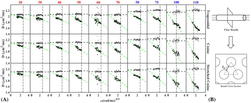
(A) Asymptotically linear dependence of D(ω) on $1/\sqrt{\omega }$ as the signature of the S/V limit is visible for all gradient waveforms, showing fits with c = 1.2. The points to the left of vertical dashed line are included in the fit. The horizontal dashed line is the value of D₀ that is fixed to the mean value of λ₁ (B) Sketch of fiber bundle cross-section for estimating typical distance between fibers, assuming strong short-range order (a triangular lattice).

Next, S/V metrics derived from diffusion modalities, equation [4], and PD modalities, equation [7], were compared via Pearson linear correlation coefficient. Additionally, Bland-Altman plots were included to emphasize differences between S/V estimates from different modalities. S/V was evaluated for at least 5 frequency points in D(ω) for the densest fiber bundle (and more points for the other bundles), corresponding to parameter c = 1.2 (as described around Eq. [8] below). The SNR was calculated using the MP-PCA method (39,40). Standard deviations for OGSE-derived parameters were obtained from the confidence interval of each fit parameter. Standard deviations for PD-derived parameters were calculated from the range of values on parametric maps.

Applicability range for the S/V limit

Since the fiber bundles have a range of packing densities, the frequency over which each individual bundle enters the S/V limit will be different. For this reason, it is important to create an objective criterion to establish the appropriate range of frequencies for parameter estimation in the S/V limit. Here we define the frequency range within the S/V limit as $\mathrm{f}\ge D_0/L_{max}^2$, where L_max is the maximal diffusion length for which the S/V limit applies.

Physically, L_max should be such that (i) it is much smaller than the distance between the fibers in the (random) packing geometry, and (ii) it is smaller than the fiber radius, since the curvature adds to the higher-order terms for the time-dependent D(t). For our purposes, since the fiber packings are quite dense and fibers are fairly similar in their radius, we define L_max in the following way: L_max = c l, where l is the geometry-dependent length scale characterizing the packing geometry (approximately treating it here as locally ordered), and c is a multiplicative factor further used for scaling l, common for all 10 phantoms.

To define the length l, consider a triangular lattice of disks of radius r, each spaced over a distance l_Δ,

$$l_{\mathrm{\Delta }}\left(r,\varphi \right)=r\left[{\left(\frac{2\pi }{3^{1/2}(1–\varphi )}\right)}^{1/2}–2\right]$$ [8]

away from one another [Fig.4(A)]. Here, ϕ is the water fraction, which can be extracted from PD measurements equation [7]. To satisfy the condition (ii) above, we then define l = min {l_Δ, r}, where $r=8.5\mu m$ is the mean fiber radius. Two fiber bundles with the highest packing density in phantom 2 had l_Δ > r [Table 3].

Table 3.

Summary of fitted parameters and other relevant physical quantities. OGSE derived values shown for c = 1.2. The cutoff frequency, f, of the S/V limit derived from SE and MRF.

	Phantom 1						Phantom 2
Bundle	20	30	40	50	60	70	50	75	100	110
TD0 (μm2/ms)	2.06±0.02	2.04±0.02	2.07±0.02	2.08±0.02	2.05±0.07	2.06±0.02	2.17±0.02	2.21±0.01	2.16±0.04	2.22±0.03
CD0 (μm2/ms)	2.09±0.01	2.08±0.01	2.11±0.02	2.11±0.02	2.09±0.08	2.09±0.02	2.20±0.02	2.23±0.03	2.18±0.04	2.24±0.04
SCD0 (μm2/ms)	2.10±0.01	2.10±0.01	2.12±0.01	2.13±0.01	2.11±0.10	2.11±0.02	2.17±0.01	2.20±0.02	2.13±0.04	2.21±0.03
TS/V (1/μm)	0.04±0.002	0.07±0.002	0.08±0.002	0.1±0.002	0.11±0.002	0.13±0.002	0.09±0.002	0.12±0.001	0.20±0.002	0.26±0.001
CS/V (1/μm)	0.05±0.002	0.07±0.002	0.09±0.002	0.11±0.002	0.12±0.002	0.13±0.001	0.10±0.002	0.13±0.002	0.21±0.003	0.28±0.013
SCS/V (1/μm)	0.04±0.002	0.06±0.009	0.07±0.002	0.10±0.009	0.12±0.007	0.13±0.002	0.10±0.002	0.13±0.002	0.20±0.002	0.28±0.013
SES/V (1/μm)	0.02±0.03	0.05±0.04	0.07±0.05	0.09±0.06	0.12±0.03	0.13±0.03	0.08±0.03	0.13±0.04	0.22±0.04	0.28±0.05
MRFS/V (1/μm)	0.03±0.03	0.05±0.04	0.07±0.06	0.11±0.05	0.13±0.02	0.14±0.02	0.10±0.02	0.15±0.03	0.23±0.03	0.31±0.04
SEφ	0.91±0.06	0.84±0.05	0.78±0.07	0.71±0.07	0.66±0.09	0.65±0.1	0.74±0.08	0.65±0.10	0.52±0.08	0.46±0.07
MRFφ	0.88±0.06	0.82±0.06	0.77±0.06	0.69±0.04	0.64±0.08	0.62±0.06	0.69±0.06	0.61±0.05	0.51±0.04	0.43±0.08
SE S/V limit [Hz] ( $\mathrm{f}\ge D0/L_{max}^2$)	22.12±0.74	22.12±0.69	22.12±1.02	22.12±1.15	22.12±1.72	22.12±1.78	22.12±1.25	22.12±1.69	39.23±3.02	64.88±5.01
MRF S/V limit ( $\mathrm{f}\ge D0/L_{max}^2$)	22.12±0.81	22.12±0.88	22.12±0.87	22.12±0.66	22.12±1.51	22.12±1.04	22.12±0.93	22.12±0.98	42.32±1.97	77.67±6.8
SElΔ (μm)	8.5	8.5	8.5	8.5	8.5	8.5	8.5	8.5	6.38±0.48	4.96±0.38
MRFlΔ (μm)	8.5	8.5	8.5	8.5	8.5	8.5	8.5	8.5	6.15±0.27	4.54±0.4
SEPoints in Fit	43	43	43	43	43	43	32	32	14	5
MRFPoints in Fit	43	43	43	43	43	43	36	36	17	6

^*Trapezoid=T, Cosine=C, Stretched Cosine=SC, Spin Echo=SE, Magnetic Resonance Fingerprinting=MRF

The multiplicative factor value c may be chosen empirically based on the quality of the fit for all samples simultaneously. We emphasize that we are not trying to achieve the best goodness of fit for each sample separately, and rather determine the objective applicability criterion for a given type of sample. We show the capability of estimating S/V as a function of c, which effectively translates to the number of points included in the fit, in Fig.5(A).

Figure 5.

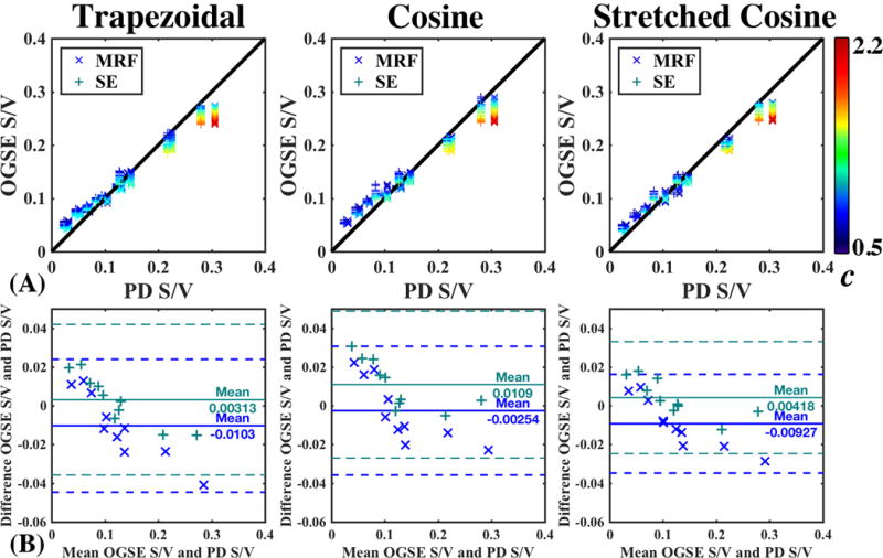
(A) Correlation plots comparing OGSE-derived S/V, Eq (1), to S/V derived from PD measurements, Eq (2), using either MRF (x) or SE (+). OGSE derived S/V as a function of c, a multiplicative factor that defines the number of points used per fit, cf. the text around Eq. (8). (B) Bland-Altman plot showing no systematic difference in S/V estimation.

Results

For the OGSE experiment, all gradient wave forms, as outputted on the scanner, are shown across one repetition time in Fig.1(A) at f = 40 Hz with N = 10, as well as the EPI train and dead time. The corresponding gradient modulation power spectra, ${\left|F(f)\right|}^2$, reveals subtle differences within the side lobes of the OGSE waveforms. The amplitude of largest off-frequency side-lobe, was smallest in for Cosine, followed by stretched cosine, and then the trapezoidal gradient waveform. The respective side-lobe amplitudes were ~[0.01, 0.5, and 1] percent of the peak resonance amplitude at 40 Hz.

Figure 2 shows the effect of the different post-processing steps (denoising/degibbsing) on a b = 0 image. Though denoising was applied and has an effect on S/V estimation (Supplementary Fig.S1), denoising has a mild visual effect on image quality, Fig.2(B). This should not be surprising as OGSE images had SNR ranging from 120–190 within the fiber bundles. By removing thermal noise, the Gibbs ringing artifact is isolated and is corrected efficiently via subvoxel shifts method, Fig.2(C).

There is a strong degree of time-dependent diffusion across all fiber bundles as demonstrated in Fig.3(A,B) showing D(t) decreasing with t ranging from a 27% to 52% drop. This contrast in D(t) is a signature of varying S/V between bundles, and is shown to increase with increasing fiber density, as determined by the number of fiber threads in the bundle. There is a visibly smoother transition between the pulse-gradient and oscillating-gradient D(t) measurements using the derived $t_{\mathrm{eff}}^{(S/V)}$, equation [6]. This is particularly true for fibers with smaller S/V (50, 75 turns), which would reach the S/V limit at lower ω. Fig.3(C,D) shows the corresponding PD-images derived from SE and PnP-MRF Fig.3(C,D), which demonstrates varying ϕ across different fiber bundles. The STEAM derived FA map at long t [Fig.3(E)], shows complementary information, with higher FA indicating greater water molecule restriction and fiber density.

Denser fibers have lower SNR due to having lower water fraction. Although the SNR is quite high, ~120 within those fibers, the b-value of this experiment is quite low. For this reason, there is notable scatter in the data, which increases with increasing S/V.

To claim accurate estimation of S/V, we evaluated whether the D(t) is acquired within the S/V limit, by showing in Fig.4(A) the characteristic asymptotically linear dependence of D(ω) on $1/\sqrt{\omega }$ according to equation [4]. For fitting, we determined a cutoff frequency, $f\ge D_0/L_{max}^2$, by considering locally ordered packing within the bundle [Fig.4(B)]. S/V values derived from the three separate OGSE measurements were highly similar [Table 3].

S/V estimates derived from SE and PnP-MRF were in strong agreement with S/V estimates from OGSE measurements ( $\rho \ge 0.99$) [Fig.5(A,B)], for c = 1.2. The range of S/V estimates increased as a function of c with increasing fiber bundle density. The mean of the differences between PD-derived and OGSE-derived S/V Bland-Altman plot did not differ significantly from 0; indicating no systematic difference between methods [Fig.5(B)]. Moreover, this result was reproducible across gradient waveforms, suggesting that S/V estimation was equally valid for each of the available OGSE variants [Table 3].

Discussion

Dispersive diffusion coefficient in a well-characterized anisotropic fiber phantom was measured using OGSE, to compare the derived S/V values with those derived from PD measurements. The geometry of our fiber phantom offers the unique capacity of measuring S/V from PD, independently from diffusion. This external measurement provides a means of validation of advanced diffusion modeling techniques including the S/V limit.

The phantom performed as anticipated (26,27): increasing the number of fibers within the bundle resulted in denser fiber bundles with a corresponding lower diffusion coefficient [Fig.3 (A,B)], decreased water fraction [Fig.3(C,D)], and higher FA [Fig.3(E)]. With increasing fiber density and S/V, the S/V limit was achieved in a shorter range of frequencies [Fig.4], as evidenced by the density-dependent range for the linear dependence of D(ω) on $1/\sqrt{\omega }$, and the increasing variation of S/V estimates when varying the range of frequencies in the fit [Fig.5(A)]. This demonstrates how applying the theory of Mitra et al. (13) outside of its applicability range will lead to systematic deviation from the ground truth S/V.

In this paper, we found no systematic difference between OGSE-derived S/V and PD-derived S/V [Fig.5(B)], suggesting that this phantom can be used as a reference standard for S/V. Although PnP-MRF is capable of separating $B_1^{+}$ heterogeneities from the PD, T₂, and T₁ maps (36), it is not able to fully account for all $B_1^{-}$ variations. The pre-scan normalize procedure uses the body coil as a reference to estimate the $B_1^{-}$ of the local receiver array. Consequently, the residual $B_1^{-}$ sensitivity variations are left in the PD map, which may be the cause of the offset. Conversely, SE is not capable of accounting for $B_1^{+}$ effects, so there may be residual bias in those images as well.

Different OGSE gradient waveforms were evaluated – including pure cosine, stretched cosine and trapezoidal, in terms of their use for clinically feasible protocols. If given the freedom to perform OGSE measurements without imaging limitations, the pure cosine gradient would be the best option as it provides the cleanest gradient modulation spectrum, ${\left|F(f)\right|}^2$. Other gradient waveforms such as stretched cosine or trapezoidal gradient inherently add higher order harmonics to ${\left|F(f)\right|}^2$, which mix different frequencies contributing to the diffusion coefficient. However, Fig.1 shows that the contribution of higher order harmonics is negligible across each waveform, suggesting that stretched cosine and trapezoidal gradients are acceptable. Since we want to probe the S/V limit, we pursue the highest possible ω for which the potential b on clinical scanners will be correspondingly low. In this experiment, we achieved b = 120 s/mm² at f = 100 Hz for a pure cosine gradient. Switching to stretched cosine or trapezoidal gradients allowed for a 33% increase, b = 160 s/mm². These relatively small b-values may be problematic when studying systems with IVIM compartments.

Cosine and stretched cosine were limited by the maximum gradient slew rate ~150 mT/m/ms. Alternatively, the trapezoidal gradient can achieve the same b-value at slew rates of 60 mT/m/ms. For this reason, the best choice of an OGSE gradient scheme for clinical translation may be the trapezoidal gradient, as the shape of this gradient results in higher b-values, compared to the other gradient forms, without any appreciable contamination by higher-order harmonics (Fig 1.). The trapezoidal gradient will be limited by peripheral nerve stimulation. The total stimulation threshold, which will prevent the sequence from running, was exceeded for slew rates higher than 60 mT/m/ms. Future OGSE projects could focus on modifying the waveform for improved feasibility on clinical systems. There have been findings that indicate it is possible to circumvent nerve stimulation limitations by greatly increasing oscillation frequency into the kHz range (43,44), which could, given hardware improvements, correspond to sensitivity towards sub-micrometer length scales.

Matching D(t) from pulsed gradients (Monopolar, STEAM) and oscillating gradients (trapezoidal, cosine, and stretched cosine) [Fig.1] showed a visually smoother transition, when using the correspondence derived in equation [6]. This suggests that for the short-time limit, the factor of 9/64 is appropriate and necessary. Studies combining PGSE and OGSE sequences have been gaining considerable popularity within the MR community (45–48). Before attempting to advance modeling towards clinical applications, it is important to understand how OGSE behaves within particular limits. This study only focused on the S/V limit. Future studies could also attempt to measure OGSE parameters within the approach of the long time (tortuosity) limit. A similar analysis of long-time limit is expected to show a different, model-specific correspondence of t and f within that limit (49), thereby allowing modeling effects of various disorder geometries (8) for both pulsed gradients and oscillating gradients for each disorder universality class.

The clinically acceptable measurement parameters of the proposed OGSE approach, demonstrated in this calibration experiment, offer an exciting perspective of mapping S/V in human subjects. In particular, this may apply for diffusion applications where the sizes of restrictions match or even exceed those of the fibers in our phantom, such as muscle (50), breast (51), and prostate (52). However, when moving to in vivo applications the D₀ is typically unknown, and may be different between multiple compartments (53).

Conclusions

In this study, we demonstrated the feasibility of performing surface-to-volume ratio estimations with a clinical whole-body 3T MR system. Our results on a well-characterized phantom can be used to calibrate OGSE acquisitions and microstructural diffusion modeling techniques, by comparing with derived parameters from non-diffusion MR modalities such as spin echo and (PnP-)MRF. Furthermore, as the measurement parameters are within a clinically acceptable range, this calibration experiment offers an exciting perspective of mapping surface-to-volume ratio in humans.

Abbreviations

ADC

Apparent Diffusion Coefficient

PGSE

Pulsed Gradient Spin Echo

OGSE

Oscillating Gradient Spin Echo

STEAM

Stimulated Echo Acquisition Mode

SE

Spin Echo

PnP-MRF

Plug-and-Play Magnetic Resonance Fingerprinting

MRF

Magnetic Resonance Fingerprinting

PD

Proton Density

DTI

Diffusion Tensor Imaging

DWI

Diffusion Weighted Image

MD

Mean Diffusivity

FA

Fractional Anisotropy

ROI

Region of Interest

EPI

Echo Planar Imaging

References

- 1.Bihan DL, Breton E, Lallemand D, Aubin ML, Vignaud J, Laval-Jeantet M. Separation of diffusion and perfusion in intravoxel incoherent motion MR imaging. Radiology. 1988;168(2):497–505. doi: 10.1148/radiology.168.2.3393671. [DOI] [PubMed] [Google Scholar]
- 2.Hagmann P, Jonasson L, Maeder P, Thiran J-P, Wedeen VJ, Meuli R. Understanding Diffusion MR Imaging Techniques: From Scalar Diffusion-weighted Imaging to Diffusion Tensor Imaging and Beyond. Radiographics: a review publication of the Radiological Society of North America, Inc. 2006;26(suppl_1):S205–S223. doi: 10.1148/rg.26si065510. [DOI] [PubMed] [Google Scholar]
- 3.Srinivasan A, Goyal M, Azri FA, Lum C. State-of-the-Art Imaging of Acute Stroke. Radiographics: a review publication of the Radiological Society of North America, Inc. 2006;26(suppl_1):S75–S95. doi: 10.1148/rg.26si065501. [DOI] [PubMed] [Google Scholar]
- 4.Padhani AR, Liu G, Mu-Koh D, Chenevert TL, Thoeny HC, Takahara T, Dzik-Jurasz A, Ross BD, Van Cauteren M, Collins D, Hammoud DA, Rustin GJS, Taouli B, Choyke PL. Diffusion-Weighted Magnetic Resonance Imaging as a Cancer Biomarker: Consensus and Recommendations. Neoplasia. 2009;11(2):102–125. doi: 10.1593/neo.81328. [DOI] [PMC free article] [PubMed] [Google Scholar]
- 5.Tanner JE. Self diffusion of water in frog muscle. Biophysical journal. 1979;28(1):107–116. doi: 10.1016/S0006-3495(79)85162-0. [DOI] [PMC free article] [PubMed] [Google Scholar]
- 6.Novikov DS, Kiselev VG. Effective medium theory of a diffusion-weighted signal. NMR Biomed. 2010;23(7):682–697. doi: 10.1002/nbm.1584. [DOI] [PubMed] [Google Scholar]
- 7.Novikov DS, Fieremans E, Jensen JH, Helpern JA. Random walk with barriers. Nature physics. 2011;7(6):508–514. doi: 10.1038/nphys1936. [DOI] [PMC free article] [PubMed] [Google Scholar]
- 8.Novikov DS, Jensen JH, Helpern JA, Fieremans E. Revealing mesoscopic structural universality with diffusion. Proceedings of the National Academy of Sciences of the United States of America. 2014;111(14):5088–5093. doi: 10.1073/pnas.1316944111. [DOI] [PMC free article] [PubMed] [Google Scholar]
- 9.Burcaw LM, Fieremans E, Novikov DS. Mesoscopic structure of neuronal tracts from time-dependent diffusion. NeuroImage. 2015;114:18–37. doi: 10.1016/j.neuroimage.2015.03.061. [DOI] [PMC free article] [PubMed] [Google Scholar]
- 10.Fieremans E, Burcaw LM, Lee H-H, Lemberskiy G, Veraart J, Novikov DS. In vivo observation and biophysical interpretation of time-dependent diffusion in human white matter. NeuroImage. 2016;129:414–427. doi: 10.1016/j.neuroimage.2016.01.018. [DOI] [PMC free article] [PubMed] [Google Scholar]
- 11.Assaf Y, Cohen Y. Non-Mono-Exponential Attenuation of Water and N-Acetyl Aspartate Signals Due to Diffusion in Brain Tissue. Journal of magnetic resonance. 1998;131(1):69–85. doi: 10.1006/jmre.1997.1313. [DOI] [PubMed] [Google Scholar]
- 12.Kim S, Chi-Fishman G, Barnett AS, Pierpaoli C. Dependence on diffusion time of apparent diffusion tensor of ex vivo calf tongue and heart. Magnetic resonance in medicine: official journal of the Society of Magnetic Resonance in Medicine / Society of Magnetic Resonance in Medicine. 2005;54(6):1387–1396. doi: 10.1002/mrm.20676. [DOI] [PubMed] [Google Scholar]
- 13.Mitra PP, Sen PN, Schwartz LM, Le Doussal P. Diffusion propagator as a probe of the structure of porous media. Physical review letters. 1992;68(24):3555–3558. doi: 10.1103/PhysRevLett.68.3555. [DOI] [PubMed] [Google Scholar]
- 14.Sen PN. Time-dependent diffusion coefficient as a probe of geometry. Concepts in Magnetic Resonance Part A. 2004;23A(1):1–21. [Google Scholar]
- 15.Latour LL, Mitra PP, Kleinberg RL, Sotak CH. Time-Dependent Diffusion Coefficient of Fluids in Porous Media as a Probe of Surface-to-Volume Ratio. Journal of Magnetic Resonance, Series A. 1993;101(3):342–346. [Google Scholar]
- 16.Mair RW, Wong GP, Hoffmann D, Hürlimann MD, Patz S, Schwartz LM, Walsworth RL. Probing Porous Media with Gas Diffusion NMR. Physical review letters. 1999;83(16):3324–3327. doi: 10.1103/PhysRevLett.83.3324. [DOI] [PubMed] [Google Scholar]
- 17.Latour LL, Svoboda K, Mitra PP, Sotak CH. Time-dependent diffusion of water in a biological model system. Proceedings of the National Academy of Sciences of the United States of America. 1994;91(4):1229–1233. doi: 10.1073/pnas.91.4.1229. [DOI] [PMC free article] [PubMed] [Google Scholar]
- 18.Gross BKR. Anwendung der spin-echo-methode der messung der selbstdiffusion. Messtechnik. 1969;77:171–7. [Google Scholar]
- 19.Stepisnik J. Analysis of NMR self-diffusion measurements by a density matrix calculation. Physica. 1981;104B(350):364. [Google Scholar]
- 20.Novikov DS, Kiselev VG. Surface-to-volume ratio with oscillating gradients. Journal of magnetic resonance. 2011;210(1):141–145. doi: 10.1016/j.jmr.2011.02.011. [DOI] [PubMed] [Google Scholar]
- 21.Parsons EC, Does MD, Gore JC. Modified oscillating gradient pulses for direct sampling of the diffusion spectrum suitable for imaging sequences. Magnetic resonance imaging. 2003;21(3–4):279–285. doi: 10.1016/s0730-725x(03)00155-3. [DOI] [PubMed] [Google Scholar]
- 22.Xu J, Li H, Harkins KD, Jiang X, Xie J, Kang H, Does MD, Gore JC. Mapping mean axon diameter and axonal volume fraction by MRI using temporal diffusion spectroscopy. NeuroImage. 2014;103:10–19. doi: 10.1016/j.neuroimage.2014.09.006. [DOI] [PMC free article] [PubMed] [Google Scholar]
- 23.Baron CA, Beaulieu C. Oscillating gradient spin-echo (OGSE) diffusion tensor imaging of the human brain. Magnetic resonance in medicine: official journal of the Society of Magnetic Resonance in Medicine / Society of Magnetic Resonance in Medicine. 2014;72(3):726–736. doi: 10.1002/mrm.24987. [DOI] [PubMed] [Google Scholar]
- 24.Reynaud O, Winters KV, Hoang DM, Wadghiri YZ, Novikov DS, Kim SG. Pulsed and oscillating gradient MRI for assessment of cell size and extracellular space (POMACE) in mouse gliomas. NMR in biomedicine. 2016;29(10):1350–1363. doi: 10.1002/nbm.3577. [DOI] [PMC free article] [PubMed] [Google Scholar]
- 25.Reynaud O, Winters KV, Hoang DM, Wadghiri YZ, Novikov DS, Kim SG. Surface-to-volume ratio mapping of tumor microstructure using oscillating gradient diffusion weighted imaging. Magnetic resonance in medicine: official journal of the Society of Magnetic Resonance in Medicine / Society of Magnetic Resonance in Medicine. 2016;76(1):237–247. doi: 10.1002/mrm.25865. [DOI] [PMC free article] [PubMed] [Google Scholar]
- 26.Fieremans E, De Deene Y, Delputte S, Özdemir MS, D’Asseler Y, Vlassenbroeck J, Deblaere K, Achten E, Lemahieu I. Simulation and experimental verification of the diffusion in an anisotropic fiber phantom. Journal of magnetic resonance. 2008;190(2):189–199. doi: 10.1016/j.jmr.2007.10.014. [DOI] [PubMed] [Google Scholar]
- 27.Fieremans E, De Deene Y, Delputte S, Ozdemir MS, Achten E, Lemahieu I. The design of anisotropic diffusion phantoms for the validation of diffusion weighted magnetic resonance imaging. Physics in medicine and biology. 2008;53(19):5405–5419. doi: 10.1088/0031-9155/53/19/009. [DOI] [PubMed] [Google Scholar]
- 28.Laun FB, Huff S, Stieltjes B. On the effects of dephasing due to local gradients in diffusion tensor imaging experiments: relevance for diffusion tensor imaging fiber phantoms. Magnetic resonance imaging. 2009;27(4):541–548. doi: 10.1016/j.mri.2008.08.011. [DOI] [PubMed] [Google Scholar]
- 29.Ianus A, Siow B, Drobnjak I, Zhang H, Alexander DC. Gaussian phase distribution approximations for oscillating gradient spin echo diffusion MRI. Journal of magnetic resonance. 2013;227:25–34. doi: 10.1016/j.jmr.2012.11.021. [DOI] [PubMed] [Google Scholar]
- 30.Van AT, Holdsworth SJ, Bammer R. In vivo investigation of restricted diffusion in the human brain with optimized oscillating diffusion gradient encoding. Magnetic resonance in medicine: official journal of the Society of Magnetic Resonance in Medicine / Society of Magnetic Resonance in Medicine. 2014;71(1):83–94. doi: 10.1002/mrm.24632. [DOI] [PMC free article] [PubMed] [Google Scholar]
- 31.Ligneul C, Valette J. Probing metabolite diffusion at ultra-short time scales in the mouse brain using optimized oscillating gradients and “short”-echo-time diffusion-weighted MRS. NMR in biomedicine. 2017;30(1) doi: 10.1002/nbm.3671. [DOI] [PMC free article] [PubMed] [Google Scholar]
- 32.Kiselev VG, Dhital B. Recipes of Diffusion Measurements with Oscillating Gradients. Proc Intl Soc Mag Reson Med. 2014;22 [Google Scholar]
- 33.Mattiello J, Basser PJ, Le Bihan D. The b matrix in diffusion tensor echo-planar imaging. Magnetic resonance in medicine: official journal of the Society of Magnetic Resonance in Medicine / Society of Magnetic Resonance in Medicine. 1997;37(2):292–300. doi: 10.1002/mrm.1910370226. [DOI] [PubMed] [Google Scholar]
- 34.Sukstanskii AL. Exact analytical results for ADC with oscillating diffusion sensitizing gradients. Journal of magnetic resonance. 2013;234:135–140. doi: 10.1016/j.jmr.2013.06.016. [DOI] [PMC free article] [PubMed] [Google Scholar]
- 35.Sigmund EE, Sui D, Ukpebor O, Baete S, Fieremans E, Babb JS, Mechlin M, Liu K, Kwon J, McGorty K, Hodnett PA, Bencardino J. Stimulated echo diffusion tensor imaging and SPAIR T2 -weighted imaging in chronic exertional compartment syndrome of the lower leg muscles. Journal of magnetic resonance imaging: JMRI. 2013;38(5):1073–1082. doi: 10.1002/jmri.24060. [DOI] [PMC free article] [PubMed] [Google Scholar]
- 36.Cloos MA, Knoll F, Zhao T, Block KT, Bruno M, Wiggins GC, Sodickson DK. Multiparametric imaging with heterogeneous radiofrequency fields. Nature communications. 2016;7:12445. doi: 10.1038/ncomms12445. [DOI] [PMC free article] [PubMed] [Google Scholar]
- 37.Ma D, Gulani V, Seiberlich N, Liu K, Sunshine JL, Duerk JL, Griswold MA. Magnetic resonance fingerprinting. Nature. 2013;495(7440):187–192. doi: 10.1038/nature11971. [DOI] [PMC free article] [PubMed] [Google Scholar]
- 38.Anderson AW. Theoretical analysis of the effects of noise on diffusion tensor imaging. Magnetic Resonance in Medicine. 2001;46(6):1174–1188. doi: 10.1002/mrm.1315. [DOI] [PubMed] [Google Scholar]
- 39.Veraart J, Novikov DS, Christiaens D, Ades-aron B, Sijbers J, Fieremans E. Denoising of diffusion MRI using random matrix theory. NeuroImage. 2016;142:394–406. doi: 10.1016/j.neuroimage.2016.08.016. [DOI] [PMC free article] [PubMed] [Google Scholar]
- 40.Veraart J, Fieremans E, Novikov DS. Diffusion MRI noise mapping using random matrix theory. Magnetic Resonance in Medicine. 2016;76(5):1582–1593. doi: 10.1002/mrm.26059. [DOI] [PMC free article] [PubMed] [Google Scholar]
- 41.Veraart J, Fieremans E, Jelescu IO, Knoll F, Novikov DS. Gibbs ringing in diffusion MRI. Magnetic resonance in medicine: official journal of the Society of Magnetic Resonance in Medicine / Society of Magnetic Resonance in Medicine. 2016;76(1):301–314. doi: 10.1002/mrm.25866. [DOI] [PMC free article] [PubMed] [Google Scholar]
- 42.Kellner E, Dhital B, Kiselev VG, Reisert M. Gibbs-ringing artifact removal based on local subvoxel-shifts. Magnetic resonance in medicine. 2016;76(5):1574–1581. doi: 10.1002/mrm.26054. [DOI] [PubMed] [Google Scholar]
- 43.Weinberg IN, Stepanov PY, Fricke ST, Probst R, Urdaneta M, Warnow D, Sanders H, Glidden SC, McMillan A, Starewicz PM, Reilly JP. Increasing the oscillation frequency of strong magnetic fields above 101 kHz significantly raises peripheral nerve excitation thresholds. Medical physics. 2012;39(5):2578–2583. doi: 10.1118/1.3702775. [DOI] [PMC free article] [PubMed] [Google Scholar]
- 44.Saritas EU, Goodwill PW, Conolly SM. Effects of pulse duration on magnetostimulation thresholds. Medical physics. 2015;42(6):3005–3012. doi: 10.1118/1.4921209. [DOI] [PMC free article] [PubMed] [Google Scholar]
- 45.Reynaud O, Winters KV, Hoang DM, Wadghiri YZ, Novikov DS, Kim SG. Surface-to-volume ratio mapping of tumor microstructure using oscillating gradient diffusion weighted imaging. Magnetic resonance in medicine: official journal of the Society of Magnetic Resonance in Medicine / Society of Magnetic Resonance in Medicine. 2015 doi: 10.1002/mrm.25865. [DOI] [PMC free article] [PubMed] [Google Scholar]
- 46.Xu J, Li H, Li K, Harkins KD, Jiang X, Xie J, Kang H, Dortch RD, Anderson AW, Does MD, Gore JC. Fast and simplified mapping of mean axon diameter using temporal diffusion spectroscopy. NMR in biomedicine. 2016 doi: 10.1002/nbm.3484. n/a-n/a. [DOI] [PMC free article] [PubMed] [Google Scholar]
- 47.Drobnjak I, Zhang H, Ianuş A, Kaden E, Alexander DC. PGSE, OGSE, and sensitivity to axon diameter in diffusion MRI: Insight from a simulation study. Magnetic Resonance in Medicine. 2016;75(2):688–700. doi: 10.1002/mrm.25631. [DOI] [PMC free article] [PubMed] [Google Scholar]
- 48.Li H, Jiang X, Xie J, McIntyre JO, Gore JC, Xu J. Time-dependent influence of cell membrane permeability on MR diffusion measurements. Magnetic Resonance in Medicine. 2015 doi: 10.1002/mrm.25724. n/a-n/a. [DOI] [PMC free article] [PubMed] [Google Scholar]
- 49.Novikov DS, Jespersen SN, Kiselev VG, Fieremans E. Quantifying brain microstructure with diffusion MRI: Theory and parameter estimation. ArXiv e-prints. 2016;1612 doi: 10.1002/nbm.3998. [DOI] [PMC free article] [PubMed] [Google Scholar]
- 50.Oudeman J, Nederveen AJ, Strijkers GJ, Maas M, Luijten PR, Froeling M. Techniques and applications of skeletal muscle diffusion tensor imaging: A review. Journal of magnetic resonance imaging: JMRI. 2016;43(4):773–788. doi: 10.1002/jmri.25016. [DOI] [PubMed] [Google Scholar]
- 51.Woodhams R, Ramadan S, Stanwell P, Sakamoto S, Hata H, Ozaki M, Kan S, Inoue Y. Diffusion-weighted Imaging of the Breast: Principles and Clinical Applications. Radiographics: a review publication of the Radiological Society of North America, Inc. 2011;31(4):1059–1084. doi: 10.1148/rg.314105160. [DOI] [PubMed] [Google Scholar]
- 52.Haider MA, van der Kwast TH, Tanguay J, Evans AJ, Hashmi A-T, Lockwood G, Trachtenberg J. Combined T2-Weighted and Diffusion-Weighted MRI for Localization of Prostate Cancer. American Journal of Roentgenology. 2007;189(2):323–328. doi: 10.2214/AJR.07.2211. [DOI] [PubMed] [Google Scholar]
- 53.Laun FB, Kuder TA, Zong F, Hertel S, Galvosas P. Symmetry of the gradient profile as second experimental dimension in the short-time expansion of the apparent diffusion coefficient as measured with NMR diffusometry. Journal of magnetic resonance. 2015;259:10–19. doi: 10.1016/j.jmr.2015.07.003. [DOI] [PubMed] [Google Scholar]
- 54.Han P, Bartels DM. Temperature Dependence of Oxygen Diffusion in H2O and D2O. The Journal of Physical Chemistry. 1996;100(13):5597–5602. [Google Scholar]
Associated Data
This section collects any data citations, data availability statements, or supplementary materials included in this article.