Mediation Analysis for Count and Zero-inflated Count Data

Abstract

Different conventional and causal approaches have been proposed for mediation analysis to better understand the mechanism of a treatment. Count and zero-inflated count data occur in biomedicine, economics and social sciences. This paper considers mediation analysis for count and zero-inflated count data under the potential outcome framework with nonlinear models. When there are post-treatment confounders which are independent of, or affected by, the treatment, we first define the direct, indirect and total effects of our interest and then discuss various conditions under which the effects of interest can be identified. Proofs are provided for the sensitivity analysis proposed in the paper. Simulation studies show that the methods work well. We apply the methods to the Detroit Dental Health Project’s Motivational Interviewing DVD (DDHP MI-DVD) trial for the direct and indirect effects of motivational interviewing on count and zero-inflated count dental caries outcomes.

1 Introduction

In many health studies, the intervention is designed to change some post-randomization (intermediate) variable, such as knowledge, attitudes, behavior, biomarkers or social factors, so that the change in the intermediate variable will lead to improvement in the final health outcomes of interest ([1]). For example, the Detroit Dental Health Project’s Motivational Interviewing DVD (DDHP MI-DVD) trial is a randomized dental trial of a Motivational Interviewing (MI) intervention to prevent early childhood caries (ECC) in low income African-American children (0 – 5 years) in Detroit, Michigan ([2]). In the study, caregivers in both intervention and control groups watched a 15-minute education video on children’s oral health. The control group (DVD only) was then provided a general recommendations on diet, oral hygiene and dental visits. For the intervention group (MI+DVD), a MI interviewer reviewed the child’s dental examination with caregivers, and discussed caregivers’ personal thoughts and concerns about specific goals for their child’s oral health. A brochure with caregivers’ specific goals was then printed and placed in a convenient place at home. Families in the MI+DVD group also received booster calls within 6 months of the intervention. The study hypothesized that the MI+DVD intervention would change the caregivers’ and children’s behaviors in oral hygiene and then the behavioral changes would lead to improved oral health in children. In these studies, researchers are not only interested if the intervention works but also if and how much the intervention affects the outcome through and around the intermediate variable. Such an intermediate variable (e.g. caregivers’ behavior change by the intervention in the DDHP MI-DVD study) is usually called a mediator and the effect of the treatment through the mediator is called indirect or mediation effect, while the effect around the mediator is called the direct effect. An indirect or mediation effect shows that the intervention affects the outcome through the intermediate variables as designed, while a direct effect indicates that the intervention changes the outcome directly or involving some other intermediate variables in a heretofore undiscovered mechanism. Knowing those effects helps us to better understand the working mechanism of an intervention such that in future research and applications in specific populations, we can tailor specific intervention components to target important mediators and consequently lead to bigger improvement in health outcomes.

Conventional mediation approaches since Baron and Kenny ([3, 4, 5]) (e.g., regression, path and structural equation model (SEM)) and recently developed causal methods ([6] – [22]) make different assumptions on the intervention and mediator to achieve a causal interpretation on the indirect (mediation) effect and direct effect of the intervention through and around a mediator. Conventional approaches model observed treatment and mediator values and may not provide a general definition/interpretation of causal effects independent of specific statistical models. Different from conventional approaches, causal mediation approaches first conceptually define causal direct and indirect effects under the potential outcome framework ([23, 24]) without reference to a specific statistical model and then different statistical models can be used to identify and estimate causal direct and indirect effects under different assumptions. Most conventional and causal approaches focus on continuous or binary outcomes. For noncontinuous outcomes such as binary outcomes with nonlinear models, MacKinnon and Dwyer ([25]) showed that the traditional product method and difference method give different results, Pearl ([7]) provided general definitions of the effects, Imai et al. ([26]) discussed general framework and inference, and VanderWeele and Vansteelandt ([15]) showed that the product method and difference method are approximately equivalent when the binary outcome is rare under assumptions.

In addition to binary outcomes, the outcome variable in many studies is often a count following a Poisson or Negative Binomial distribution, or a zero-inflated count that has a higher probability of being zero than expected under a Poisson or Negative Binomial, such as number of doctor or emergency visits, number of admissions and readmissions to a hospital, number of complications, and number of decayed, missing and filled teeth (dmft) or tooth surfaces (dmfs). The dental outcomes of interest in the DDHP MI-DVD study are the number of new untreated lesions, dmft and dmfs at the end of the study 2 years later compared to the DVD group ([2]). Since the majority of the children did not have any new untreated lesions, dmft and dmfs at the end of the study, the distributions of the outcomes contain a lot of zeros (Figure 2). In this paper, we will examine whether or not the intervention did change caregivers’ behavior regarding their children’s oral health (e.g. parents made sure their children brush teeth) as designed and whether or not the behavioral changes had an effect on children’s oral health with a mediation analysis.

Figure 2.

Histograms of the numbers of new untreated cavities, new dmfs and new dmft in participants at 2 years in DDHP MI-DVD study26

Assuming a Poisson or Negative Binomial (NB) distribution on dental outcomes such as dmft and dmfs, Albert and Nelson ([27]) developed a nice approach for estimating different pathway effects based on the potential outcome framework ([8]) in the context of a directed acyclic graph (DAG) using generalized linear models, Albert ([28]) considered an inverse-probability weighted estimator for the mediation effect on count outcomes, and Valeri and Vander Weele ([29]) provided formula for the direct and indirect effects on the rate ratio scale when the mediator is continuous. Assuming a zero-inflated negative binomial (ZINB) model for the outcome, Wang and Albert ([30]) provided a mediation formula for the mediation effect estimation in a two-stage model and considered a decomposition of the mediation effect in a three-stage model when there is no post-treatment confounder. In this paper, we will use the same definitions and general framework as previous work ([7], [15], [26], [27]) but we are interested in the overall direct, mediation (indirect) and total effects specifically for count (Poisson and NB) and zero-inflated count (zero-inflated Poisson or ZIP, and zero-inflated negative binomial or ZINB) data. And as in other work on mediation on nonlinear models ([7], [15], [26], [27]), we will have the direct effects depend on the level of the mediating variable and the indirect effects depend on the level of the treatment variable. In this paper, we will particularly consider cases when there are post-treatment confounders (independent of or affected by treatment) in a study with count and zero-inflated count data. Various conditions, in addition to Albert and Nelson’s conditional independence assumption ([27]), will be discussed to identify the effects of our interest with theoretical proofs. A sensitivity analysis will then be proposed under the cases when there is post-treatment confounding (see Section 4 for detailed discussion).

The rest of the paper is organized as follows. In Section 2, we set up the causal framework, introduce notation and assumptions, and define the indirect and direct effects. In Section 3, we extend the method to estimate the indirect and direct effect in randomized trials with count or zero-inflated count outcomes. In Section 4, we present some simulation studies. An application of our method to the DDHP MI-DVD study is shown in Section 5. Finally, we provide conclusions and discussion in Section 6.

All the programming used and analyses conducted in this paper were written in R (https://cran.r-project.org/) and are available from the authors.

2 The Framework

In this study, we will use the potential (counterfactual) outcome framework ([23, 24]) to specify the direct, indirect (mediation) and overall effects of the treatment. We will make the Stable Unit Treatment Value Assumption (SUTVA) in the paper. SUTVA says that a subject’s potential outcome is not related to the randomization or mediation value of other subjects or the method of administration of randomization or the mediator. Under SUTVA, we use Z_i to denote the treatment variable, M_i for the observed mediator level, X_i for the observed baseline covariates and Y_i for observed outcome for subject i. In a two-arm trial, Z_i = 1 if subject i is randomized to the intervention group and Z_i = 0 if randomized to the control group. We let $M_i^z$ denote the potential value of a mediator under treatment Z_i = z for subject i, which has two versions $M_i^1$ under intervention and $M_i^0$ under control. However, in practice we are not able to observe both potential mediator values but only one of $M_i^1$ and $M_i^0$ depending on which treatment group subject i was actually assigned to. We use $Y_i^{z,m}$ to denote the potential outcome subject i would have under the treatment Z_i = z and mediator M_i = m, and $Y_i^{z,M_i^z}$ for potential outcome under Z_i = z, where $Y_i^{z,m}$ will be used below to define controlled effects and $Y_i^{z,M_i^z}$ for natural effects. Again, we can only observe one version of multiple potential outcomes for a subject depending on the actual treatment and mediator value subject i had.

The total effect (TE) or intent-to-treat (ITT) effect of the intervention and its average are

$$TE=Y_i^{1,M_i^1}-Y_i^{0,M_i^0},\mathit{TE}=E(Y_i^{1,M_i^1}-Y_i^{0,M_i^0}),$$

which is the total effect of the intervention (Z = 1) on outcome Y compared to control (Z = 0) no matter whether the effect is through or around mediator M. The total or ITT effect of the intervention has two components: the effect of the intervention around the mediator, called the direct effect, and the effect of the intervention through the mediator, called the indirect or mediation effect. Two sets of definitions on these effects have been proposed in the literature ([7, 9, 17, 31, 32]): controlled and natural effects.

The controlled direct effect (CDE) of the intervention and its average while fixing the mediator at m are

$$CD{E}_m=Y_i^{1m}-Y_i^{0m},C\overline{D}{E}_m=E(Y_i^{1m}-Y_i^{0m}),$$

which is the effect of intervention compared to control while fixing the mediator at m; and the controlled mediation effect (CME) of m vs. m′ when fixing z and its average are

$$\begin{array}{c}CM{E}_z=Y_i^{zm}-{Y_i^{zm}}^{\prime },C\overline{M}{E}_z=E(Y_i^{zm}-Y_i^{z{m}^{\prime }}),\\ \text{for}z=0,1\text{and}\text{all}m\ne m^{\prime },\end{array}$$

which is the effect of mediator (at m vs. at m′) on the outcome under treatment z.

Alternatively, instead of setting the mediator at a fixed level m in the controlled effects, the natural effects set the mediator at its “natural” level that would be achieved under treatment assignment z. The natural direct effect (NDE) of intervention and its average when the mediator is set at its level under treatment assignment z are

$$ND{E}_z=Y_i^{1,M_i^z}-Y_i^{0,M_i^z},N\overline{D}{E}_z=E(Y_i^{1,M_i^z}-Y_i^{0,M_i^z}),$$

which is the effect of intervention on outcome compared to control while having the mediator at its potential level $M_i^z$; and the natural mediation (indirect) effect (NME) and its average when fixing treatment z are

$$NM{E}_z=Y_i^{z,M_i^1}-Y_i^{z,M_i^0},N\overline{M}{E}_z=E(Y_i^{z,M_i^1}-Y_i^{z,M_i^0}),$$

which is the outcome change under treatment z that would be observed if the mediator would change from the value under control $M_i^0$ to the value under treatment $M_i^1$. In some studies, natural effects are probably preferred since we may not be able to set the mediator at a specific level. However, stronger assumptions are often needed to identify natural effects than controlled effects since the potential outcome corresponding to both levels of Z, $Y_i^{z,M_i^{z^{\prime }}}(z\ne z^{\prime })$, is involved in natural effects. In this paper, we will focus on the natural effects while the controlled effects will be mentioned in the discussion of existing approaches.

3 Mediation Analysis for Count and Zero-inflated Count Data

As discussed above, the counterfactual potential outcome involved in the natural effects $Y_i^{z,M_i^{z^{\prime }}}(z\ne z^{\prime })$ is not observed. To identify the effects, we assume sequential ignorability as per Imai et al ([17, 26]):

$$\{Y_i^{z^{\prime },m},M_i^z\}\perp Z_i|X_i=x;Y_i^{z^{\prime },m}\perp M_i^z|Z_i=z,X_i=x,\text{for}\text{all}z,z^{\prime },m.$$ (1)

This assumption says that (a) given the baseline covariates, the treatment is independent of potential mediators and potential outcomes; and (b) given the treatment and baseline covariates, the mediators are independent of the potential outcomes. In the DVD-MI study, the first ignorability assumption is reasonable because participants were randomized to the MI intervention. The random assignment of the intervention does not guarantee the second ignorability assumption because the oral health behavior after randomization was not randomly assigned. However, the second ignorability assumption may hold after conditioning on baseline covariates and treatment; that is, the oral health behavior was as if randomized among subjects in the same treatment group who have the same baseline characteristics.

Under sequential ignorability, Imai, Keele and Tingley ([26]) showed that the distribution of the potential outcome is nonparametrically identified, i.e., the distribution of the potential outcome on the left hand side can be expressed as a function of the distribution of observed data on the right hand side:

$$f(Y_i^{z,M_i^{z^{\prime }}}|X_i=x)={\displaystyle {\int }_{M}f(Y_i|M_i=m,Z_i=z,X_i=x)d{F}_{M_i}(m|Z_i=z^{\prime },X_i=x),x\in X;z,z^{\prime }}=0,1.$$ (2)

This result allows us to estimate the potential outcome and mediators we do not observe. Based on this result, we further assume the following mediator and outcome models:

$$\begin{array}{rrr}\hfill M_i^{Z_i}& \hfill \sim & \hfill f_M({\theta }_M=h^{-1}({\alpha }_M+{\beta }_M{Z}_i+{\eta }_M^T{X}_i))\end{array}$$ (3)

$$\begin{array}{rrr}\hfill Y_i^{Z_i,M_i^{Z_i}}& \hfill \sim & \hfill f_Y({\theta }_Y=g^{-1}({\alpha }_Y+{\beta }_Y{Z}_i+{\gamma }_Y{M}_i^{Z_i}+{\xi }_Y{Z}_i{M}_i^{Z_i}+{\eta }_Y^T{X}_i))\end{array}$$ (4)

where the link functions h and g are monotonic and differentiable functions; e.g., identity link for normally distributed M_i or Y_i, and probit link for binary M_i or Y_i. For a count outcome or mediator following a Poisson or Negative Binomial distribution, a loglinear model can be used as per Albert and Nelson ([27]). For zero-inflated outcomes, different approaches ([33]) have been proposed outside the mediation context. In this paper, we will adopt the zero-inflated Poisson (ZIP) ([34]) or zero-inflated Negative Binomial (ZINB) ([35]) model for zero-inflated counts in the mediation context. The basic idea of these models is that the outcome is a mixture of zeros and Poisson (or Negative Binomial) random variables with the mixture proportion $p(Z_i,M_i^{Z_i},X_i)$ and Poisson (or Negative Binomial) mean $\lambda (Z_i,M_i^{Z_i},X_i)$ depending on the covariates X_i. When an interpretation only relies on the second part (positive outcome) of the ZIP or ZINB model, the conclusion could be misleading because the two groups with the positive outcome are not ensured to be comparable by randomization ([36]). In this paper, our estimates of direct, mediation and total effects and their comparisons between groups will use information from all the randomized subjects with both parts of the model so that the ignorability of randomization holds. The outcome distribution under ZIP is:

$$\begin{array}{l}P(Y_i^{Z_i,M_i^{Z_i}}=0)={\omega }_i+(1-{\omega }_i)e^{-{\lambda }_i};\\ P(Y_i^{Z_i,M_i^{Z_i}}=j)=(1-{\omega }_i)\frac{e^{-{\lambda }_i}{\lambda }_i^j}{j!};j>0\end{array}$$ (5)

while the outcome distribution under ZINB is:

$$\begin{array}{l}P(Y_i^{Z_i,M_i^{Z_i}}=0)={\omega }_i+(1-{\omega }_i){(1+\sigma {\lambda }_i)}^{-\frac{1}{\sigma }};\\ P(Y_i^{Z_i,M_i^{Z_i}}=j)=(1-{\omega }_i)\frac{\mathrm{\Gamma }(j+\frac{1}{\sigma })}{j!\mathrm{\Gamma }(\frac{1}{\sigma })}{(\sigma {\lambda }_i)}^j{(1+\sigma {\lambda }_i)}^{-j-\frac{1}{\sigma }};j>0\end{array}$$ (6)

where

$$\begin{array}{l}\log \frac{{\omega }_i}{1-{\omega }_i}={\alpha }_{Y1}+{\beta }_{Y1}{Z}_i+{\gamma }_{Y1}{M}_i^{Z_i}+{\xi }_{Y1}{Z}_i{M}_i^{Z_i}+{\eta }_{Y1}^T{X}_i,\\ \log {\lambda }_i={\alpha }_{Y2}+{\beta }_{Y2}{Z}_i+{\gamma }_{Y2}{M}_i^{Z_i}+{\xi }_{Y2}{Z}_i{M}_i^{Z_i}+{\eta }_{Y2}^T{X}_i\end{array}$$ (7)

σ(≥ 0) is a dispersion parameter that does not depend on covariates.

Then as in Imai et al. ([17, 26]), the procedure based on the quasi-Bayesian Monte Carlo approximation of King, Tomz, and Wittenberg ([37]) will be used to make inference on the direct and indirect effects of treatment:

1. Fit the mediator and outcome models with observed mediator and outcome, and obtain estimated parameters (coefficients) and their estimated asymptotic covariance matrix.

2. Simulate model parameters (coefficients) from their sampling distribution based on the approximate multivariate normal distribution with mean and variance equal to the estimated parameters (coefficients) and their estimated asymptotic covariance matrix obtained in (I), and sample J copies of the mediator and outcome model coefficients from their sampling distributions: ${\theta }_M^j$ and ${\theta }_Y^j$.

3. For each copy j = 1, …, J, repeat the following steps:

   1. simulate potential values of the mediator under each z = 0, 1 for each subject based on the mediator model (3) with simulated parameters (coefficients) obtained in (II);
   2. simulate potential outcomes under each z = 0, 1 for each subject based on the outcome model (4) with simulated potential mediator values obtained in (a) and simulated parameters (coefficients) obtained in (II);
   3. compute the direct, mediation and total treatment effects by averaging the difference between the corresponding two predicted potential outcomes discussed in Section 2.

4. Compute the point estimates of direct, mediation and total effects, confidence intervals and p values based on the results from J repetitions. We use the sample median, standard deviation, and percentiles of the corresponding distributions from the J repetitions as the point estimate, standard error and confidence interval for the direct, indirect (mediation) and total effects.

4 Mediation Analysis with Post Treatment Confounders

In Section 3, we only consider situations with measured baseline confounders X_i. In this section, we will consider mediation analysis for cases with some confounding after randomization. For example, in the DDHP MI-DVD study, when we evaluate the effect of the MI+DVD intervention on children’s dental outcomes around or through whether or not caregivers made sure their child brushed at bedtime, caregivers’ oral hygiene knowledge and their own behaviors after randomization could be associated with both whether or not they made sure their child brushed and children’s dental outcomes and therefore are post-treatment confounders for the mediation analysis of our interest.

We let U_i denote post-treatment confounders. Figure 1 shows the treatment mechanism through and around the mediator when the treatment (a) does not affect and (b) does affect the post-treatment confounder, respectively.

Figure 1.

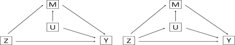
Treatment mechanism when Z does not affect U (a) and when Z affects U (b)

4.1 Post Treatment Confounders not Affected by the Treatment

When the post-treatment confounder U_i is not affected by treatment Z_i (Figure 1(a)), average natural effects are identified ([32]) under the sequential ignorability (8):

$$(Y_i^{z^{\prime },m},M_i^Z)\perp Z_i|X_i=x;\text{and}{Y}_i^{z^{\prime },m}\perp M_i^z|Z_i=z,X_i=x,U_i=u,\text{for}\text{all}z,z^{\prime },m,u.$$ (8)

The first part of (8) is the same as the first part of (1), which says that the treatment is randomly assigned conditional on X_i. The second part of (8) is similar to the second part of (1) except that now the ignorability of the mediator holds given not only the treatment assignment and baseline covariates but also post-treatment confounders. That is, the mediator is effectively random (independent of confounding) among subjects in the same treatment group who have the same values of baseline characteristics and post-treatment confounders.

To estimate the direct and indirect natural effects of the treatment when the post-treatment confounder U_i is not affected by treatment Z_i, we can modify the outcome model by including the post-treatment confounder in the model:

$$Y_i^{Z_i,M_i^{Z_i}}\sim f_Y({\theta }_Y=g^{-1}({\alpha }_Y+{\beta }_Y{Z}_i+{\gamma }_Y{M}_i^{Z_i}+{\eta }_Y^T{X}_i+{\varphi }_Y^T{U}_i))$$ (9)

Then the same procedure discussed in Section 3 can be used for the estimation of direct and indirect natural effects. For zero-inflated count data, (7) changes to

$$\begin{array}{l}\log \frac{{\omega }_i}{1-{\omega }_i}={\alpha }_{Y1}+{\beta }_{Y1}{Z}_i+{\gamma }_{Y1}{M}_i^{Z_i}+{\eta }_{Y1}^T{X}_i+{\varphi }_{Y1}^T{U}_i,\\ \log {\lambda }_i={\alpha }_{Y2}+{\beta }_{Y2}{Z}_i+{\gamma }_{Y2}{M}_i^{Z_i}+{\eta }_{Y2}^T{X}_i+{\varphi }_{Y2}^T{U}_i\end{array}$$

4.2 Post Treatment Confounders Affected by the Treatment

When treatment Z_i affects the post-treatment confounder U_i (Figure 1(b)), average natural effects are not identified under assumption (8) without additional information. Instead, average controlled effects can be estimated under sequential ignorability (8) and the extended outcome model (10):

$$Y_i^{Z_i,M_i}\sim f_Y({\theta }_Y=g^{-1}({\alpha }_Y+{\beta }_Y{Z}_i+{\gamma }_Y{M}_i+{\eta }_Y^T{X}_i+{\varphi }^T{U}_i)).$$ (10)

The average controlled mediation effect can be estimated by a function of ${\widehat{\gamma }}_Y$, but the estimate of the average controlled direct effect by ${\widehat{\beta }}_Y$ could be biased ([32]) because U_i is also affected by Z_i and the effect through U_i is not incorporated in the estimation of the controlled direct effect. For continuous outcomes with an identity link function in (10), Vansteelandt ([38]) and Joffe and Greene ([39]) used a two-stage ordinary least squares (OLS) procedure to estimate the average controlled direct effect by correcting the bias in the second stage. Some researchers considered the derivation of bounds for the natural direct and indirect effects ([40, 41, 42]). Tchetgen Tchetgen and Shpitser ([43]) and VanderWeele and Chiba ([44]) considered various contrasts of the outcome between two subpopulations as sensitivity parameters and then corrected the bias with specified values of sensitivity parameters. Tchetgen Tchetgen and VanderWeele ([45]) assumed monotonicity about the effect of the treatment (exposure) on the confounder and showed the nonparametrical identifiability of the natural direct effect. For binary mediators, Taguri and Chiba ([46]) classified subjects into four principal M-response strata and estimated the natural direct and indirect effects under additional monotonicity assumption on treatment-mediator effect and assumption of common average mediator effects between compliant and never intermediates.

In this section, we will consider a sensitivity analysis for the direct and indirect effects on count and zero-inflated count outcomes when the treatment affects the post-treatment confounder. We consider the average natural mediation, direct and total effects as:

$$\begin{array}{l}N\overline{M}{E}_z=E\left(Y_i^{z,U_i^z,M_i^{1,U_i^1}}-Y_i^{z,U_i^z,M_i^{0,U_i^0}}\right),\mathrm{for}z=0,1\\ N\overline{D}{E}_z=E\left(Y_i^{1,U_i^1,M_i^{z,U_i^z}}-Y_i^{0,U_i^0,M_i^{z,U_i^z}}\right),\mathrm{for}z=0,1\\ N\overline{T}E=E\left(Y_i^{1,U_i^1,M_i^{1,U_i^1}}-Y_i^{0,U_i^0,M_i^{0,U_i^0}}\right)=N\overline{D}{E}_1+N\overline{M}{E}_0.\end{array}$$ (11)

It is easy to derive that the total natural effect is the sum of natural direct effect under treatment and natural mediation effect under control similar as Wang and Albert ([28]) and Imai et al. ([26]). We consider the mediation effect as the causal effect of the treatment on the outcome through the mediator M under treatment z; and the direct effect as all other causal effects of the treatment on the outcome around M, including the effect through the post-treatment confounder U. That is, the confounding effect is included in the direct effect when it is not the interest. Please see Daniel et al. ([47]) for discussion on various approaches when more than one intermediate variables exist in a study. When effects through different intermediate variables are the interest of investigators, Imai and Yamamoto ([48]) assumed a linear structural equation model for the outcome and mediators and estimated the effects, Daniel et al. ([47]) considered the finest possible decomposition of the total effect, and VanderWeele and Vansteelandt ([49]) considered the mediators one at a time as joint mediators and proposed decomposition of the total effect with regression-based and weighting approaches. For count data, Albert and Nelson ([27]) assumed independence between one mediator under treatment Z₁(1) and under control Z₁(0) and then conduct a sensitivity analysis on pathway effects. In this section, we will consider other practical assumptions in addition to the conditional independence assumption, under which the direct and indirect effects are identified. We will also provide theoretical proofs for the effect identification, and then propose sensitivity analyses under those assumptions.

We assume sequential ignorability (12) and (13) and mediator and outcome models:

$$\left(Y_i^{z,u,m},M_i^{z^{\prime },u^{\prime }},U_i^z\right)\perp Z_i|X_i=x$$ (12)

$$Y_i^{z,u,m}\perp M_i^{z^{\prime },u^{\prime }}|X_i=x,Z_i=z,U_i^z=u$$ (13)

$$M_i^{Z_i}\sim f_M({\theta }_M=h^{-1}({\alpha }_M+{\beta }_M{Z}_i+{\varphi }_M{U}_i^{Z_i}+{\eta }_M^T{X}_i))$$ (14)

$$Y_i^{Zi,M_i^{Z_i}}\sim f_Y({\theta }_Y=g^{-1}({\alpha }_Y+{\beta }_Y{Z}_i+{\gamma }_Y{M}_i^{Z_i}+{\varphi }_Y{U}_i^{Z_i}+{\eta }_Y^T{X}_i))$$ (15)

Additionally, we assume various models below for the post-treatment confounder $U_i^{Z_i}$ Then we can show that the effects (11) are identified under (12) – (15) and one of (16) – (18).

$$U_i^1=U_i^0+{\beta }_U,$$ (16)

$$U_i^1=U_i^0+{\beta }_U+{\tau }_U^T{X}_i,$$ (17)

$$\begin{array}{l}{U}_i^1=U_i^0+{\beta }_U+{\tau }_U^T{X}_i+{\delta }_i,\text{where}{\delta }_i\perp (Z_i,X_i,U_i^0,Y_i^{z,u,m},M_i^{z^{\prime },u^{\prime }})\\ \text{and}{\delta }_i\text{follows}\mathrm{a}\text{known}\text{distribution}\end{array}$$ (18)

Models (16) – (18) are good for continuous post-treatment confounders, where Model (18) allows the heterogeneity treatment effect on U for individuals. For a binary confounder U, one can also assume an underlying continuous variable following one of Models (16) – (18). For general post-treatment confounders, we assume the following set of assumptions to identify the effects (11),

$$\left(Y_i^{z,u,m},M_i^{z^{\prime },u^{\prime }},U_i^1,U_i^0\right)\perp Z_i|X_i=x$$ (19)

$$Y_i^{z,u,m}\perp M_i^{z^{\prime },u^{\prime }}|X_i=x,Z_i=z,U_i^0=u,U_i^1=u^{\prime }$$ (20)

and

$$\begin{array}{l}{U}_i^{Z_i}\sim f_U({\theta }_U=o^{-1}({\alpha }_U+{\beta }_U{Z}_i+{\tau }_U^T{X}_i)),\\ U_i^1\perp U_i^0|X_i=x\mathrm{and}\left(Y_i^{z,u,m},M_i^{z^{\prime },u^{\prime }}\right)\perp (U_i^0,U_i^1)|X_i=x,Z_i=z\end{array}$$ (21)

Note that (19) and (20) are slightly different from the assumptions (12) and (13) since (19) and (20) are involved with joint distribution of $(U_i^0,U_i^1)$ while (12) and (13) are only involved with marginal distribution $U_i^z$. In practice, if the ignorability holds for marginal distribution $U_i^z$, it is reasonable to assume that the ignorability also holds for the joint distribution $U_i^1$ and $U_i^0$. Assumption (21) is the similar as the conditional independence assumption on Z₁(1) and Z₀(0) in Albert and Nelson ([27]), however, instead of assuming independence between U¹ and U⁰, Assumptions (16) – (18) assume some relation between U¹ and U⁰ and could be more practical in some real studies.

Result 1

Given sequential ignorability (12) and (13), mediator model (14) and outcome model (15), and one of confounder models (16) – (18), then the average effects $N\overline{M}{E}_z$, $N\overline{D}{E}_z$ and $N\overline{T}{E}_z$ are identified. Given sequential ignorability (13),(19) and (20), mediator model (14) and outcome model (15), and the confounder model (21), then the average effects $N\overline{M}{E}_z$, $N\overline{D}{E}_z$ and $N\overline{T}{E}_z$ are identified.

Please see the Appendix for the proof. Note that Model (21) works for general post-treatment confounders, and Result 1 also holds when the interaction $Z_i\times U_i^{Z_i}$ is included in the mediator model (14) and interactions $Z_i\times M_i^{Z_i}$ and $Z_i\times U_i^{Z_i}$ are included in the outcome model (15). The procedure based on the quasi-Bayesian Monte Carlo approximation ([37]) discussed in Section 3 can then be used for inference on the direct, mediation and total treatment effects but with one additional confounder model (16), (17), (18) or (21).

In a real study, we can conduct a sensitivity analysis by varying the values of parameters β_U and ${\tau }_U^T$ one or two at a time and see how the estimates of effects (11) will change. Although we are not able to know the values of those parameters for sure, information from the study is helpful for specifying values of those parameters under sequential ignorability (12) and (13) or (19) and (20). Estimates from a regression of observed U_i on treatment Z_i, covariates X_i and their interaction can provide reasonable starting points for the choice of values for β_U and ${\tau }_U^T$ in the sensitivity analysis. For example, in U_i = α_U + δ_UZ_i + ν_UX_i + ε_i, ${\widehat{\delta }}_U$ would be a reasonable starting value for β_U in (16). We suggest to use the estimated value based on observables ± c% (say $\frac{1}{3}$, 50% or 100%) of the estimated value as a range for the parameters, where the choice of c% will be based on expert knowledge in a study such that the range will represent the possible treatment effect on the confounder. Then equally divided 10–20 values in the range can be used for the sensitivity analysis.

5 Simulation Studies

In this section, we will present simulation studies to examine the finite sample performance of the methods discussed in Sections 3 and 4.

The treatment Z_i was assigned randomly with a probability of 0.5 to either treatment or control group. The baseline covariates were drawn independently from N(0, 1), Bernoulli(0.5), and/or multinomial((1, 2, 3, 4), (0.25, 0.25, 0.25, 0.25)). The results are similar with different types of covariates and only results with the normal and binary covariates are reported. We consider both continuous and binary mediators:

$$M_i^{Z_i}\sim N({\alpha }_M+{\beta }_M{Z}_i+{\eta }_M^T{X}_i,1);M_i^{Z_i}\sim \mathit{Binary}(\frac{\exp ({\alpha }_M+{\beta }_M{Z}_i+{\eta }_M^T{X}_i)}{1+\exp ({\alpha }_M+{\beta }_M{Z}_i+{\eta }_M^T{X}_i)})$$

Four families of outcome distributions were considered in the simulation studies: Poisson (Poi), Negative Binomial (NB), Zero-inflated Poisson (ZIP) and Zero-inflated Negative Binomial (ZINB).

$$\begin{array}{l}{Y}_i^{Z_i,M_i^{Z_i}}\sim \mathit{Poi}(\exp [{\alpha }_Y+{\beta }_Y{Z}_i+({\gamma }_Y+\delta Z_i)M_i^{Z_i}+{\eta }_Y^T{X}_i])\\ Y_i^{Z_i,M_i^{Z_i}}\sim NB(\exp [{\alpha }_Y+{\beta }_Y{Z}_i+({\gamma }_Y+\delta Z_i)M_i^{Z_i}+{\eta }_Y^T{X}_i],\mathit{size}=c)\\ Y_i^{Z_i,M_i^{Z_i}}=0\text{with}{p}_i=\mathit{expit}\{{\alpha }_Y+{\beta }_Y{Z}_i+({\gamma }_Y+\delta Z_i)M_i^{Z_i}+{\eta }_Y^T{X}_i\};\\ \sim \mathit{Poi}(\exp [{\alpha }_Y+{\beta }_Y{Z}_i+({\gamma }_Y+\delta Z_i)M_i^{Z_i}+{\eta }_Y^T{X}_i])\text{with}(1-p_i).\\ Y_i^{Z_i,M_i^{Z_i}}=0\text{with}{p}_i=\mathit{expit}\{{\alpha }_Y+{\beta }_Y{Z}_i+({\gamma }_Y+\delta Z_i)M_i^{Z_i}+{\eta }_Y^T{X}_i\};\\ \sim NB(\exp [{\alpha }_Y+{\beta }_Y{Z}_i+({\gamma }_Y+\delta Z_i)M_i^{Z_i}+{\eta }_Y^T{X}_i],\mathit{size}=c)\text{with}(1-p_i).\end{array}$$

The true values of the coefficients are not presented in this paper to save space but are available from the authors. Instead, the true values of NDE, NME and NTE are included in Tables 1 and 2. Basically the coefficient values were selected such that there would be about 20% zeroes for Poisson and negative binomial data and about 50% zeroes for ZIP and ZINB data to represent the common data structure in real dental studies (see Figure 2). For each distribution family, we simulated one setting where the treatment affected the outcome and about 30% of its effect was through the mediator seen in some real studies ([50]), and another setting corresponding to the null hypothesis of no direct and indirect effects. For each setting, we performed 1, 000 Monte Carlo replications, generating data for 100 and 500 subjects respectively on each replication.

Table 1.

Simulation results without post-treatment confounders

D’n	M	N	Z	NDE	$N\widehat{D}E$	NDE RMSE	Cov.	$r\widehat{r}$	NME	$N\widehat{M}E$	NME RMSE	Cov.	$r\widehat{r}$	NTE	$N\widehat{T}E$	NTE RMSE	Cov.	$r\widehat{r}$
Poi	N	100	1	1.641	1.656	0.019	98.3	0.979	0.647	0.662	0.018	94.3	0.690	1.915	1.947	0.035	98.8	0.999
			0	1.268	1.286	0.020	98.0	0.978	0.273	0.291	0.019	94.1	0.485
		500	1	1.644	1.643	0.005	98.9	1.000	0.652	0.656	0.006	94.8	1.000	1.916	1.919	0.006	98.7	1.000
			0	1.264	1.263	0.004	98.6	1.000	0.273	0.276	0.004	94.8	1.000
	B	100	1	1.517	1.504	0.018	98.8	0.959	0.464	0.451	0.018	99.8	0.104	1.813	1.792	0.026	99.3	0.933
			0	1.349	1.341	0.013	97.9	0.946	0.297	0.289	0.011	99.1	0.104
		500	1	1.519	1.512	0.008	99.1	1.000	0.481	0.478	0.006	99.9	0.605	1.823	1.816	0.009	99.7	1.000
			0	1.342	1.339	0.006	99.0	1.000	0.304	0.304	0.004	99.6	0.605
NB	N	100	1	1.513	1.551	0.043	95.0	0.725	0.699	0.724	0.028	95.6	0.508	1.935	2.002	0.070	96.0	0.900
			0	1.236	1.278	0.045	94.5	0.725	0.422	0.451	0.030	94.6	0.508
		500	1	1.511	1.533	0.024	96.2	1.000	0.695	0.701	0.008	93.6	0.992	1.932	1.958	0.028	96.6	1.000
			0	1.238	1.258	0.021	94.8	1.000	0.421	0.425	0.005	92.4	0.992
	B	100	1	1.513	1.554	0.047	96.1	0.547	0.471	0.471	0.013	98.4	0.094	1.804	1.852	0.055	97.6	0.628
			0	1.333	1.382	0.054	95.5	0.532	0.290	0.299	0.012	95.9	0.092
		500	1	1.524	1.519	0.012	96.8	0.994	0.469	0.458	0.013	98.1	0.555	1.821	1.811	0.015	98.5	1.000
			0	1.353	1.354	0.009	96.0	0.996	0.297	0.292	0.006	95.7	0.555
ZIP	N	100	1	1.608	1.667	0.063	99.9	0.544	0.675	0.675	0.014	96.2	0.295	1.920	1.953	0.039	99.9	0.896
			0	1.244	1.278	0.038	99.1	0.581	0.312	0.285	0.028	99.3	0.036
		500	1	1.600	1.591	0.015	99.9	0.996	0.662	0.636	0.027	95.3	0.890	1.908	1.865	0.045	99.6	1.000
			0	1.247	1.229	0.020	98.5	0.996	0.308	0.274	0.034	98.3	0.391
	B	100	1	1.539	1.565	0.037	99.2	0.501	0.510	0.498	0.016	91.4	0.129	1.848	1.879	0.040	99.9	0.688
			0	1.338	1.381	0.048	98.6	0.498	0.309	0.313	0.007	94.0	0.118
		500	1	1.507	1.500	0.015	99.3	0.986	0.497	0.488	0.010	88.9	0.989	1.810	1.814	0.014	99.8	1.000
			0	1.313	1.326	0.017	98.6	0.993	0.303	0.314	0.012	94.3	0.989
ZINB	N	100	1	1.614	1.706	0.099	99.9	0.548	0.525	0.532	0.017	93.1	0.291	1.886	1.958	0.083	99.8	0.786
			0	1.361	1.425	0.072	99.2	0.605	0.272	0.252	0.022	96.8	0.099
		500	1	1.626	1.626	0.032	99.7	0.984	0.538	0.522	0.020	93.3	0.963	1.888	1.880	0.038	99.6	0.993
			0	1.350	1.358	0.027	98.8	0.988	0.263	0.253	0.011	96.6	0.799
	B	100	1	1.603	1.614	0.044	99.1	0.421	0.548	0.537	0.021	95.9	0.130	1.942	1.954	0.049	99.8	0.563
			0	1.394	1.417	0.043	98.8	0.402	0.340	0.340	0.012	97.2	0.140
		500	1	1.535	1.525	0.035	99.3	0.942	0.520	0.524	0.013	96.6	0.883	1.859	1.864	0.040	99.5	0.983
			0	1.339	1.340	0.029	98.9	0.930	0.324	0.339	0.017	96.6	0.878

D’n: distribution; M: mediator; N: sample size; NDE: natural direct effect; NME: natural mediation effect; NTE: natural total effect; RMSE: root mean squared error; Cov: 95% CI coverage; rr: empirical rejection rate of the test; Poi: Poisson, NB: negative binomial; ZIP: zero-inflated Poisson; ZINB: zero-inflated negative binomial; N: normal; B: binary

Table 2.

Simulation results with a post-treatment confounder

D’n	M	N	Z	NDE	$N\widehat{D}E$	NDE RMSE	Cov.	$r\widehat{r}$	NME	$N\widehat{M}E$	NME RMSE	Cov.	$r\widehat{r}$	NTE	$N\widehat{T}E$	NTE RMSE	Cov.	$r\widehat{r}$
Poi	N	100	1	0.706	0.702	0.011	97.0	0.605	0.260	0.262	0.006	98.7	0.354	0.828	0.844	0.018	97.8	0.792
			0	0.568	0.582	0.016	97.2	0.571	0.122	0.142	0.020	95.3	0.199
		500	1	0.709	0.704	0.006	95.1	1.000	0.264	0.258	0.007	98.7	0.950	0.833	0.834	0.004	96.7	1.000
			0	0.569	0.576	0.008	95.5	1.000	0.124	0.130	0.006	93.9	0.950
	B	100	1	0.721	0.710	0.016	96.8	0.430	0.307	0.279	0.029	93.8	0.412	0.907	0.900	0.013	97.3	0.664
			0	0.600	0.622	0.025	96.7	0.376	0.186	0.190	0.005	90.9	0.456
		500	1	0.721	0.714	0.009	97.8	0.991	0.313	0.300	0.013	95.2	1.000	0.910	0.909	0.005	98.1	1.000
			0	0.598	0.609	0.013	96.9	0.982	0.189	0.195	0.007	92.8	1.000
NB	N	100	1	0.696	0.709	0.018	97.1	0.363	0.252	0.267	0.017	96.3	0.246	0.817	0.854	0.039	97.6	0.548
			0	0.565	0.587	0.024	96.2	0.336	0.120	0.145	0.025	93.6	0.113
		500	1	0.698	0.699	0.005	98.0	0.982	0.253	0.251	0.004	95.6	0.934	0.820	0.829	0.010	98.3	0.998
			0	0.566	0.578	0.013	98.1	0.983	0.122	0.130	0.008	91.7	0.920
	B	100	1	0.756	0.752	0.016	95.0	0.319	0.262	0.234	0.029	91.4	0.185	0.908	0.906	0.015	97.2	0.471
			0	0.647	0.672	0.029	96.2	0.283	0.152	0.154	0.004	89.8	0.222
		500	1	0.751	0.743	0.011	99.0	0.949	0.252	0.239	0.013	87.7	0.938	0.899	0.892	0.009	99.1	0.997
			0	0.647	0.653	0.008	98.4	0.933	0.147	0.150	0.003	84.6	0.929
ZIP	N	100	1	0.760	0.700	0.061	99.0	0.129	0.309	0.252	0.057	80.5	0.144	0.897	0.866	0.035	99.0	0.248
			0	0.589	0.614	0.028	97.9	0.125	0.138	0.167	0.028	89.3	0.088
		500	1	0.765	0.656	0.109	95.4	0.790	0.295	0.220	0.076	70.5	0.706	0.902	0.798	0.104	95.7	0.955
			0	0.607	0.579	0.029	95.7	0.846	0.138	0.142	0.005	81.2	0.704
	B	100	1	0.889	0.826	0.065	99.6	0.210	0.317	0.295	0.023	87.0	0.092	1.084	1.030	0.056	99.6	0.414
			0	0.767	0.736	0.034	99.3	0.192	0.195	0.204	0.010	93.3	0.201
		500	1	0.915	0.809	0.106	97.8	0.902	0.331	0.291	0.040	85.2	0.985	1.106	1.011	0.096	98.2	0.988
			0	0.776	0.720	0.056	98.9	0.905	0.192	0.202	0.010	87.5	0.991
ZINB	N	100	1	0.853	0.834	0.032	99.1	0.123	0.414	0.400	0.019	87.4	0.181	1.091	1.076	0.030	99.7	0.353
			0	0.677	0.676	0.018	99.0	0.165	0.238	0.242	0.010	89.0	0.073
		500	1	0.830	0.761	0.070	98.2	0.659	0.411	0.333	0.079	84.6	0.708	1.062	0.961	0.103	98.5	0.917
			0	0.651	0.628	0.026	97.2	0.787	0.232	0.200	0.033	84.5	0.432
	B	100	1	0.829	0.817	0.074	99.1	0.133	0.365	0.217	0.198	91.3	0.051	1.067	1.079	0.075	99.2	0.253
			0	0.702	0.861	0.257	99.0	0.106	0.238	0.262	0.025	94.4	0.093
		500	1	0.809	0.741	0.071	98.2	0.570	0.372	0.337	0.036	87.8	0.874	1.066	0.993	0.077	98.3	0.869
			0	0.695	0.656	0.042	97.7	0.600	0.258	0.252	0.007	92.6	0.924

D’n: distribution; M: mediator; N: sample size; NDE: natural direct effect; NME: natural mediation effect; NTE: natural total effect; RMSE: root mean squared error; Cov: 95% CI coverage; rr: empirical rejection rate of the test; Poi: Poisson, NB: negative binomial; ZIP: zero-inflated Poisson; ZINB: zero-inflated negative binomial; N: normal; B: binary

In the simulation for cases with a post-treatment confounder affected by the treatment, we consider and present results from one normal U model with a normal covariate but other U models work similarly.

$$U_i^0\sim N({\alpha }_U+{\eta }_U^T{X}_i,{\sigma }_{\epsilon }^2),U_i^1=U_i^0+{\beta }_U;$$

The corresponding mediator and outcome models are:

$$\begin{array}{l}{M}_i^{Z_i}\sim N({\alpha }_M+{\beta }_M{Z}_i++{\varphi }_M{U}_i^{Z_i}+{\eta }_M^T{X}_i,1);\\ M_i^{Z_i}\sim \mathit{Binary}(\frac{\exp ({\alpha }_M+{\beta }_M{Z}_i+{\varphi }_M{U}_i^{Z_i}+{\eta }_M^T{X}_i)}{1+\exp ({\alpha }_M+{\beta }_M{Z}_i+{\varphi }_M{U}_i^{Z_i}+{\eta }_M^T{X}_i)})\\ Y_i^{Z_i,M_i^{Z_i}}\sim \mathit{Poi}(\exp [{\alpha }_Y+{\beta }_Y{Z}_i+{\gamma }_Y{M}_i^{Z_i}+{\varphi }_Y{U}_i^{Z_i}+{\eta }_Y^T{X}_i])\\ Y_i^{Z_i,M_i^{Z_i}}\sim NB(\exp [{\alpha }_Y+{\beta }_Y{Z}_i+{\gamma }_Y{M}_i^{Z_i}+{\varphi }_Y{U}_i^{Z_i}+{\eta }_Y^T{X}_i],\mathit{size}=c)\\ Y_i^{Z_i,M_i^{Z_i}}=0\text{with}{p}_i=\mathit{expit}\{{\alpha }_Y+{\beta }_Y{Z}_i+{\gamma }_Y{M}_i^{Z_i}+{\varphi }_Y{U}_i^{Z_i}+{\eta }_Y^T{X}_i\};\\ \sim \mathit{Poi}(\exp [{\alpha }_Y+{\beta }_Y{Z}_i+{\gamma }_Y{M}_i^{Z_i}+{\varphi }_Y{U}_i^{Z_i}+{\eta }_Y^T{X}_i])\text{with}(1-p_i).\\ Y_i^{Z_i,M_i^{Z_i}}=0\text{with}{p}_i=\mathit{expit}\{{\alpha }_Y+{\beta }_Y{Z}_i+{\gamma }_Y{M}_i^{Z_i}+{\varphi }_Y{U}_i^{Z_i}+{\eta }_Y^T{X}_i\};\\ \sim NB(\exp [{\alpha }_Y+{\beta }_Y{Z}_i+{\gamma }_Y{M}_i^{Z_i}+{\varphi }_Y{U}_i^{Z_i}+{\eta }_Y^T{X}_i],\mathit{size}=c)\text{with}(1-p_i).\end{array}$$

The true values of natural direct, indirect (mediation) and total effects were computed as the average difference between two corresponding potential outcomes with the true values of the parameters (coefficients). The average estimated values, root mean squared errors (RMSE), confidence interval coverages, and empirical rejection rates for a level of 0.05 are shown in Tables 1 and 2 without and with the post-treatment confounder (from (16)) respectively when there are direct and mediation effects (the alternative hypothesis is true). We can see that the bias and RMSEs are small under all outcome distributions with and without post treatment confounders. The 95% confidence interval coverage is good for most cases, but when there is a post-treatment confounder affected by the treatment, the coverage is less than 95% for the mediation effect for ZIP and ZINB, where around 40%–70% observations are zero. The test has higher power to detect direct and total effects than the power to detect mediation effects, and the power to detect the mediation effect is increased when the sample size is increased from 100 to 500. A more detailed investigation on the power will be performed in a future study. When there are no direct and indirect effects (the null hypothesis is true), the pattern of results is similar with Type I error < 0.05 for all cases (The results are not shown to save space).

6 Application

In this section, we will conduct an analysis on the DDHP MI-DVD trial ([2]) with the method discussed in this paper. In the study, 790 families (0–5 years old children and their caregivers) were randomly assigned to one of two education groups (DVD only or MI+DVD). In addition to watching a special 15-minute DVD on how the caregivers could help their children stay free from tooth decay, families in the intervention group (MI+DVD) met a MI interviewer, developed their own preventive goals, and received booster calls within 6 months of the intervention. Table 3 shows the baseline characteristics of participants by randomization assignment. The two groups were balanced in age, gender, caregiver education, household income, soda consumption, dental visit, tooth brushing, and dental outcomes at baseline.

Table 3.

Baseline characteristics by randomization assignment

	MI + DVD (n=370)	DVD only (n=364)
Child characteristics
Age	4.6 ± 1.6	4.5±1.7
Gender
Female	197(53.2%)	194(53.3%)
Soda consumption
Never	117(36.2%)	112(36.6%)
1 day/week	28(8.7%)	35(11.4%)
2–6 days/week	127(39.3%)	124(40.5%)
Every day	51(15.8%)	35(11.4%)
Dental visit in the past 2 years	249(67.3%)	236(64.8%)
Number of times child brushed	1.66 ± 0.78	1.66 ± 0.95
Untreated cavities	3.0 ± 5.9	2.9 ± 5.7
dmfs	9.2 ± 10.5	8.8 ± 10.2
dmft	5.3 ± 8.8	5.0 ± 8.3
Caregiver/family characteristics
Age	31.6 ± 8.8	31.0 ± 9.2
Gender
Female	355(95.9%)	344(94.5%)
Education
Less than high school	179(48.4%)	151(41.5%)
High school/GED	114(30.8%)	126(34.6%)
Some college or more	77(20.8%)	87(23.9%)
Household income
< $10K	156(42.2%)	139(38.2%)
$10K ∼	105(28.4%)	97(26.7%)
$20K ∼	63(17.0%)	71(19.5%)
$30K ∼	46(12.4%)	57(15.7%)
Made sure child brushed at bedtime
$Yes	229 (61.9%)	219 (60.2%)

The dental outcomes of interest include the number of new untreated lesions, number of decayed, missing and filled surfaces (dmfs) and number of decayed, missing and filled teeth (dmft) at 2 years. The number of new untreated lesions, dmfs and dmft took values of integers and had around 60%, 26% and 47% zeros respectively. Figure 2 shows the dental outcome histograms by group at two years. Table 4 shows the results from ordinary analyses on the randomized trial. Compared to the oral health at baseline, both groups had decreased number of new untreated lesions, slightly increased dmfs and similar dmft at 2 years. A logistic regression was used to model the mediator whether or not caregivers made sure their child brushed at bedtime on intervention, showing that caregivers in the MI+DVD group were significantly more likely to make sure their child brushed at bedtime at 6 months than caregivers in the DVD only group (p value=0.0178). Log linear models for Negative Binomial data were then fitted to model the dental outcomes at 2 years on the intervention, mediator and their interactions. It is shown that there was no significant difference in dental outcomes between the MI+DVD and DVD only groups and no significant difference in dental outcomes between caregivers who made sure and did not make sure their child brushed at bedtime.

Table 4.

Intervention effects on children’s dental outcomes by conventional analysis

Variable	MI+DVD	DVD only	P value
Caregiver made sure child brush at bedtime at 6m	304 (82.16%)	273 (74.91%)	0.0178
New untreated lesion at 2 years
Made sure child brush at bedtime at 6m	1.88 ± 3.74	1.93 ± 3.95	0.8887
Didn’t make sure child brush at bedtime at 6m	2.45 ± 6.68	1.58 ± 2.95	0.2151
P value	0.3678	0.4581
dmfs at 2 years
Made sure child brush at bedtime at 6m	10.77 ± 11.45	10.07 ± 10.63	0.5574
Didn’t make sure child brush at bedtime at 6m	11.17 ± 11.08	11.18 ± 11.51	0.9970
P value	0.8471	0.5315
dmft at 2 years
Made sure child brush at bedtime at 6m	5.03 ± 8.05	4.67 ± 7.30	0.6546
Didn’t make sure child brush at bedtime at 6m	4.67 ± 8.50	4.64 ± 7.20	0.9842
P value	0.7814	0.9763

To examine whether or not the behavioral change (e.g. parents made sure their children brushed teeth) by the intervention had an effect on children’s oral health and whether or not the intervention had a direct effect on children’s oral health around this behavior change, we will use methods discussed in this paper to examine the direct and indirect effect of the intervention on the dental outcomes around or through caregivers’ behavior to make sure their child brushed at bedtime at 6 months. In this study, the ignorability of treatment is satisfied because of randomization. Then we will first conduct a mediation analysis assuming that the ignorability of mediator is plausible after controlling for relevant baseline covariates, and we will next conduct a sensitivity analysis assuming that there is some post-treatment confounding on the mediator-outcome relation to see how the results will change. We will control for relevant baseline covariates such as soda consumption, household income, caregivers’ education, number of times child brushed, whether or not caregivers made sure their child brushed, whether or not caregivers provided child healthy meals, and dental visits at baseline. The ignorability of the mediator implies that among those children who were assigned to the same group and had the same baseline characteristics, whether or not caregivers made sure their child brushed at bedtime at 6 months were not associated with confounders. Some empirical work has advocated conditioning on many exogenous covariates to make a variable more plausibly unrelated with confounding (see [51], [52] among others). Assuming no post-treatment confounding first, Poisson, Negative Binomial, zero-inflated Poisson and zero-inflated Negative Binomial outcome models were fitted for the dental outcomes)number of new untreated cavities, new dmfs and new dmft at two years) with intervention, mediator, and baseline covariates included in the models. The Vuong test ([53]) was used to compare different outcome models and showed that the zero-inflated Negative Binomial outcome models were preferred. Table 5 shows the estimated direct, indirect (mediation) and total effects for the three dental outcomes. None of the direct, mediation and total effects were significant, indicating no significant evidence that the effect of the MI+DVD intervention on caregivers making sure children brushed at bedtime translated to an improvement of dental outcomes at 2 years.

Table 5.

Direct and indirect effects of the MI+DVD intervention on children’s dental outcomes

Dental Outcome	Direct Effect		Mediation Effect		Total Effect
	Estimate (95% CI)	P	Estimate (95% CI)	P	Estimate (95% CI)	P
New untreated lesion	0.007 (−0.666, 0.696)	0.99	−0.001 (−0.053, 0.050)	0.96	0.0006 (−0.665, 0.709)	0.99
dmfs	0.381 (−1.076, 1.770)	0.63	−0.045 (−0.219, 0.058)	0.46	0.335 (−1.135, 1.736)	0.66
dmft	0.114 (−1.070, 1.234)	0.83	0.020 (−0.057, 0.134)	0.77	0.134 (−1.069, 1.237)	0.81

When we evaluate the effect of the MI+DVD intervention on children’s dental outcomes around or through whether or not caregivers made sure their child brushed at bedtime, we note that the MI+DVD intervention could also affect caregivers’ oral hygiene knowledge and other behaviors on oral hygiene, which could be associated with both whether or not they made sure their child brushed at bedtime and their child’s dental outcomes. That is, there could be some post-treatment confounding on the mediator-outcome relationship. Therefore, we conduct a sensitivity analysis with methods discussed in Section 4.2 to see how the results will change. Specifically we modeled a post-treatment confounder (dental visits in the follow-up) on the treatment and baseline covariates. The estimated intervention effect on the confounder was −0.15, that is, the intervention had a small effect in reducing dental visits based on observed data. Although we do not know the real β_U in Models (16) – (18) and (21) because we are not able to observe $U_i^1$ and $U_i^0$ simultaneously, we use a reasonable range for β_U based on the observed intervention effect on the confounder for sensitivity analyses. Specifically we use −0.15 ± $\frac{1}{3}$ (−0.15), i.e., (−0.20, −0.10) as the reasonable range for β_U in terms of possible intervention effect on the confounder. Figure 3 shows that with various values of β_U, the mediation effects stay around 0 while the direct and total effects increase and vary within a range from 0.03 for untreated cavities to 0.15 for dmfs. That is, given that the intervention affected an intermediate confounder (dental visits) at different levels, the mediation effect of the MI+DVD intervention via caregivers making sure their child brushed at bedtime stays no effect on children’s dental outcomes, and the direct effect of the MI+DVD on the dental outcomes around caregivers making sure their child brushed at bedtime is increased compared to the direct effect given no post-treatment confounding shown in Table 5 but the effect is not significant (p values > 0.05).

Figure 3.

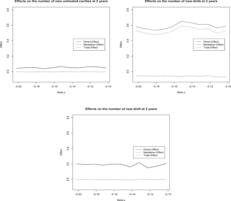
Sensitivity analysis for direct, mediation and total effects on the numbers of new untreated cavities, new dmfs and new dmft with varying treatment effects on the post treatment confounder β_U

In summary, the MI+DVD intervention significantly increased the likelihood of caregivers making sure their child brushed at bedtime at 6 months but this effect on caregivers’ behavior did not lead to improved dental outcomes at 2 years compared to DVD only. Future studies will be needed to design an intervention for behavioral changes leading to improved dental outcomes.

7 Discussion

This paper considers mediation analysis for count and zero-inflated count outcomes – common outcomes in dental studies and other fields. Sequential ignorability is assumed in the methods discussed in this paper. Although the mediator is not randomly assigned such that the ignorability of the mediator is not guaranteed, the assumption is more likely satisfied after controlling for relevant baseline covariates. See [51], [52] among others for empirical work showing that conditioning on many covariates makes a variable more plausibly unrelated with confounding. When we evaluate the direct and mediation effects of the treatment through a mediator of interest, it is common that there are some other intermediate variables, which are affected by treatment and also associated with the outcome and mediator of interest, so called post-treatment confounders. Those post-treatment confounders make the evaluation of natural direct and mediation effects difficult. In this paper, we consider mediation sensitivity analysis with the presence of post-treatment confounders by modeling the post-treatment confounders on treatment and baseline covariates along with quasi-Bayesian Monte Carlo approximation based g-computation. This method allows us to evaluate the natural direct and mediation effects with sensitivity parameters easily specified.

In addition to the dental outcomes discussed in this paper, healthcare utilizations such as the number of doctor visits or emergency visits and number of admissions and readmissions to a hospital, and medical outcomes such as the number of complications, are often count or zero-inflated count data. The methods discussed in this paper can be applied to those data. Important baseline confounders should be controlled in the mediator and outcome models such that the sequential ignorability is a reasonable assumption. When there is a concern of a post-treatment confounder which is affected by the treatment, sensitivity analysis proposed in this paper should be considered to see how the results will change while the sensitivity parameters vary in a realistic range in the study.

Appendix

Proof of Result 1

To estimate the natural direct and indirect effect, it is essential to estimate $E\left(Y_i^{0,U_i^0,M_i^{1,U_i^1}}\right)$, $E\left(Y_i^{1,U_i^1,M_i^{1,U_i^1}}\right)$ and $E\left(Y_i^{0,U_i^0,M_i^{0,U_i^0}}\right)$. Let F_Z (·) and F_Z|W (·) represent the distribution function of a random variable Z and the conditional distribution function of Z given W.

Note that

$$\begin{array}{l}E\left(Y_i^{0,U_i^0,M_i^{0,U_i^0}}\right)\\ ={\displaystyle \int E\left(Y_i^{0,U_i^0,M_i^{0,U_i^0}}|X_i=x\right)d{F}_{X_i}\left(x\right)}\\ ={\displaystyle \int E\left(Y_i^{0,u,M_i^{0,u}}|X_i=x,U_i^0=u\right)d{F}_{U_i^0|X_i=x}\left(u\right)d{F}_{X_i}\left(x\right)}\\ ={\displaystyle \int E\left(Y_i^{0,u,m}|X_i=x,U_i^0=u,M_i^{0,u}=m\right)d{F}_{M_i^{0,u}|X_i=x,U_i^0=u}\left(m\right)d{F}_{U_i^0|X_i=x}\left(u\right)d{F}_{X_i}\left(x\right)}.\end{array}$$ (22)

By the ignorability assumption (12), we have

$$\begin{array}{l}E(Y_i^{0,u,m}|X_i=x,U_i^0=u,M_i^{0,u}=m)=E(Y_i^{0,u,m}|X_i=x,Z_i=0,U_i^0=u,M_i^{0,u}=m)\\ =E(Y_i|X_i=x,Z_i=0,U_i=u,M_i=m),\end{array}$$ (23)

and

$$\begin{array}{l}d{F}_{M_i^{0,u}|X_i=x,U_i^0=u}\left(m\right)=d{F}_{M_i^{0,u}|X_i=x,Z_i=0,U_i^0=u}\left(m\right)=d{F}_{Mi|X_i=x,Z_i=0,U_i=u}\left(m\right),\\ d{F}_{U_i^0|X_i=x}\left(u\right)=d{F}_{U_i^0|X_i=x,Z_i=0}\left(u\right)=d{F}_{U_i|X_i=x,Z_i=0}\left(u\right).\end{array}$$ (24)

By combining (22), (23) and (24), we have

$$\begin{array}{l}E\left(Y_i^{0,U_i^0,M_i^{0,U_i^0}}\right)={\displaystyle \int E\left(Y_i|X_i=x,Z_i=0,U_i=u,M_i=m\right)}\\ d{F}_{M_i|X_i=x,Z_i=0,U_i=u}\left(m\right)d{F}_{U_i|X_i=x,Z_i=0}\left(u\right)d{F}_{X_i}\left(x\right).\end{array}$$ (25)

Similarly, we can also obtain

$$\begin{array}{l}E\left(Y_i^{1,U_i^1,M_i^{1,U_i^1}}\right)={\displaystyle \int E\left(Y_i|X_i=x,Z_i=1,U_i=u,M_i=m\right)}\\ d{F}_{M_i|X_i=x,Z_i=1,U_i=u}\left(m\right)d{F}_{U_i|X_i=x,Z_i=1}\left(u\right)d{F}_{X_i}\left(x\right).\end{array}$$ (26)

In the following, we identify the counterfactual outcome $E\left(Y_i^{0,U_i^0,M_i^{1,U_i^1}}\right)$. Note that

$$\begin{array}{l}E\left(Y_i^{0,U_i^0,M_i^{1,U_i^1}}\right)\\ ={\displaystyle \int E\left(Y_i^{0,U_i^0,M_i^{1,U_i^1}}|X_i=x\right)d{F}_{X_i}\left(x\right)}\\ ={\displaystyle \int E\left(Y_i^{0,u,M_i^{1,U_i^1}}|X_i=x,U_i^0=u\right)d{F}_{U_i^0|X_i=x}\left(u\right)d{F}_{X_i}\left(x\right)}\\ ={\displaystyle \int E\left(Y_i^{0,u,M_i^{1,u^{\prime }}}|X_i=x,U_i^0=u,U_i^1=u^{\prime }\right)d{F}_{U_i^1|X_i=x,U_i^0=u}(u^{\prime })d{F}_{U_i^0|X_i=x}\left(u\right)d{F}_{X_i}\left(x\right)}\\ ={\displaystyle \int E\left(Y_i^{0,u,m}|X_i=x,U_i^0=u,U_i^1=u^{\prime },M_i^{1,u^{\prime }}=m\right)}\\ d{F}_{M_i^{1,u^{\prime }}|U_i^1=u^{\prime },X_i=x,U_i^0=u}d{F}_{U_i^1|X_i=x,U_i^0=u}(u^{\prime })d{F}_{U_i^0|X_i=x}\left(u\right)d{F}_{X_i}\left(x\right).\end{array}$$ (27)

Proof under Model (16)

By (16), we have

$$d{F}_{U_i^1|X_i=x,U_i^0=u}(u^{\prime })=1_{u^{\prime }=u+{\beta }_U},$$ (28)

where 1_u′=_u+βU is the indicator function taking value 1 when u^′ = u + β_U and value 0 on all other places. Hence, (27) can be expressed as

$$\begin{array}{l}E\left(Y_i^{0,U_i^0,M_i^{1,U_i^1}}\right)={\displaystyle \int E\left(Y_i^{0,u,m}|X_i=x,U_i^0=u,M_i^{1,u+{\beta }_U}=m\right)}\\ d{F}_{M_i^{1,u+{\beta }_U}|U_i^1=u+{\beta }_U,X_i=x}d{F}_{U_i^0|X_i=x}\left(u\right)d{F}_{X_i}\left(x\right)\end{array}$$ (29)

Note that

$$d{F}_{U_i^0|X_i=x}\left(u\right)=d{F}_{U_i|X_i=x,Z_i=0}\left(u\right).$$

The remaining goal is to identify the following quantities,

$$E\left(Y_i^{0,u,m}|X_i=x,U_i^0=u,M_i^{1,u+{\beta }_U}=m\right),$$ (30)

and

$$d{F}_{M_i^{1,u+{\beta }_U}|U_i^1=u+{\beta }_U,X_i=x}.$$ (31)

By (12), we have

$$\begin{array}{l}d{F}_{M_i^{1,u+{\beta }_U}|U_i^1=u+{\beta }_U,X_i=x}=d{F}_{M_i^{1,u+{\beta }_U}|X_i=x,Z_i=1,U_i^1=u+{\beta }_U}\left(m\right)\\ =d{F}_{M_i|X_i=x,Z_i=1,U_i=u+{\beta }_U}\left(m\right).\end{array}$$ (32)

For the conditional expectation part, we have

$$\begin{array}{l}E\left(Y_i^{0,u,m}|X_i=x,U_i^0=u,M_i^{1,u+{\beta }_U}=m\right)\\ =E\left(Y_i^{0,u,m}|X_i=x,Z_i=0,U_i^0=u,M_i^{1,u+{\beta }_U}=m\right)\\ =E\left(Y_i^{0,u,m}|X_i=x,Z_i=0,U_i^0=u\right)\\ =E\left(Y_i^{0,u,m}|X_i=x,Z_i=0,U_i^0=u,M_i^{0,u}=m\right)\\ =E\left(Y_i|X_i=x,Z_i=0,U_i=u,M_i=m\right),\end{array}$$ (33)

where the first equality follows from (12) and the second and third equalities follow from (13). Combing (28), (32) and (33), (27) can be expressed as

$$\begin{array}{l}E\left(Y_i^{0,U_i^0,M_i^{1,U_i^1}}\right)={\displaystyle \int E\left(Y_i|X_i=x,Z_i=0,U_i=u,M_i=m\right)}\\ d{F}_{M_i|X_i=x,Z_i=1,U_i=u+{\beta }_U}\left(m\right)d{F}_{U_i|X_i=x,Z_i=0}\left(u\right)d{F}_{X_i}\left(x\right).\end{array}$$ (34)

Proof under Model (17)

All the results under Model (16) hold by replacing β_U with ${\beta }_U+{\tau }_U^{T}x$.

Proof under Model (18)

By (27), we have

$$\begin{array}{l}E\left(Y_i^{0,U_i^0,M_i^{1,U_i^1}}\right)\\ ={\displaystyle \int E\left(Y_i^{0,u,M_i^{1,u^{\prime }}}|X_i=x,U_i^0=u,U_i^1=u^{\prime }\right)d{F}_{U_i^1|X_i=x,U_i^0=u}\left(u^{\prime }\right)d{F}_{U_i^0|X_i=x}\left(u\right)d{F}_{X_i}\left(x\right)}\\ ={\displaystyle \int E\left(Y_i^{0,u,M_i^{1,u+{\beta }_U+{\tau }_U^{T}x+\delta }}|X_i=x,U_i^0=u,U_i^1=u+{\beta }_U+{\tau }_U^{T}x+\delta \right)d{F}_{{\delta }_i}\left(\delta \right)d{F}_{U_i^0|X_i=x}\left(u\right)d{F}_{X_i}\left(x\right)}\\ ={\displaystyle \int E\left(Y_i^{0,u,m}|X_i=x,U_i^0=u,U_i^1=u+{\beta }_U+{\tau }_U^{T}x+\delta ,M_i^{1,u+{\beta }_U+{\tau }_U^{T}x+\delta }=m\right)}\\ d{F}_{M_i^{1,u+{\beta }_U+{\tau }_U^{T}x+\delta }|U_i^1=u,{\beta }_U+{\tau }_U^{T}x+\delta ,X_i=x,U_i^0=u}d{F}_{{\delta }_i}\left(\delta \right)d{F}_{U_i^0|X_i=x}\left(u\right)d{F}_{X_i}\left(x\right).\end{array}$$ (35)

By the assumption ${\delta }_i\perp (Z_i,X_i,U_i^0,Y_i^{z,u,m},M_i^{z^{\prime }.u^{\prime }})$, we have

$$\begin{array}{l}E\left(Y_i^{0,U_i^0,M_i^{1,U_i^1}}\right)={\displaystyle \int E\left(Y_i|X_i=x,Z_i=0,U_i=u,M_i=m\right)}\\ d{F}_{M_i|X_i=x,Z_i=1,U_i=u+{\beta }_U+{\tau }_U^{T}x+\delta }\left(m\right)d{F}_{{\delta }_i}\left(\delta \right)d{F}_{U_i|X_i=x,Z_i=0}\left(u\right)d{F}_{X_i}\left(x\right).\end{array}$$ (36)

Proof under Model (21)

By (21), we have

$$d{F}_{U_i^1|X_i=x,U_i^0=u}(u^{\prime })=d{F}_{U_i^1|X_i=x}(u^{\prime })=d{F}_{U_i|X_i=x,Z_i=1}(u^{\prime }).$$

By (20), we have

$$\begin{array}{l}d{F}_{M_i^{1,u^{\prime }}|X_i=x,U_i^0=u,U_i^1=u^{\prime }}\left(m\right)=d{F}_{M_i^{1,u^{\prime }}|X_i=x,Z_i=1,U_i^0=u,U_i^1=u^{\prime }}\left(m\right)=d{F}_{M_i^{1,u^{\prime }}|X_i=x,Z_i=1}\left(m\right)\\ =d{F}_{M_i^{1,u^{\prime }}|X_i=x,Z_i=1,U_i^1=u^{\prime }}=d{F}_{M_i|X_i=x,Z_i=1\text{'}{U}_i{u}^{\prime }}\left(m\right).\end{array}$$

Note that

$$\begin{array}{l}E\left(Y_i^{0,u,m}|X_i=x,U_i^0=u,U_i^1=u^{\prime },M_i^{1,u^{\prime }}=m\right)\\ =E\left(Y_i^{0,u,m}|X_i=x,Z_i=0,U_i^0=u,U_i^1=u^{\prime },M_i^{1,u^{\prime }}=m\right)\\ =E\left(Y_i^{0,u,m}|X_i=x,Z_i=0,U_i^0=u,U_i^1=u^{\prime }\right)\\ =E\left(Y_i^{0,u,m}|X_i=x,Z_i=0\right)\\ =E\left(Y_i^{0,u,m}|X_i=x,Z_i=0,U_i^0=u\right)\\ =E\left(Y_i^{0,u,m}|X_i=x,Z_i=0,U_i^0=u,M_i^{0,u}=m\right)\\ =E\left(Y_i|X_i=x,Z_i=0,U_i=u,M_i=m\right),\end{array}$$

where the first equality follows from (19), the second and the forth equality follow from (20) and the third equality follows from (13). Then,

$$\begin{array}{l}E\left(Y_i^{0,U_i^0,M_i^{1,U_i^1}}\right)={\displaystyle \int E\left(Y_i|X_i=x,Z_i=0,U_i=u,M_i=m\right)}\\ d{F}_{M_i|X_i=x,Z_i=1,U_i=u^{\prime }}\left(m\right)d{F}_{U_i|X_i=x,Z_i=1}(u^{\prime })d{F}_{U_i|X_i=x,Z_i=0}\left(u\right)d{F}_{X_i}\left(x\right)\end{array}$$

References

- 1.MacKinnon DP, Luecen LJ. Statistical analysis for identifying mediating variables in public health dentistry interventions. Journal of Public Health Dentistry. 2011;71(Suppl 1):S37–46. doi: 10.1111/j.1752-7325.2011.00252.x. [DOI] [PMC free article] [PubMed] [Google Scholar]
- 2.Ismail AI, Ondersma S, Willem Jedele JM, Little RJ, Lepkowski JM. Evaluation of a brief tailored motivational intervention to prevent early childhood caries. Community Dentistry and Oral Epidemiology. 2011;39:433–448. doi: 10.1111/j.1600-0528.2011.00613.x. [DOI] [PMC free article] [PubMed] [Google Scholar]
- 3.Baron RM, Kenny DA. The moderator-mediator variable distinction in social psychological research: conceptual, strategic, and statistical considerations. Journal of Personality and Social Psychology. 1986;51:1173–1182. doi: 10.1037//0022-3514.51.6.1173. [DOI] [PubMed] [Google Scholar]
- 4.Cole DA, Maxwell SE. Testing mediation models with longitudinal data: Questions and tips in the use of structural equation modeling. Journal of Abnormal Psychology. 2003;112:558–577. doi: 10.1037/0021-843X.112.4.558. [DOI] [PubMed] [Google Scholar]
- 5.MacKinnon DP. Introduction to Statistical Mediation Analysis. New York: Erlbaum; 2008. [Google Scholar]
- 6.Robins JM, Greenland S. Identifiability and exchangeability for direct and indirect effects. Epidemiology. 1992;3:143–155. doi: 10.1097/00001648-199203000-00013. [DOI] [PubMed] [Google Scholar]
- 7.Pearl J. Direct and indirect effects. In: Breese J, Koller D, editors. Proceedings of the 17th Conference on Uncertainty in Artificial Intelligence. San Francisco, CA: Morgan Kaufmann; 2001. [Google Scholar]
- 8.Rubin D. Direct and indirect causal effects via potential outcomes. Scandinavian Journal of Statistics. 2004;31:161–170. [Google Scholar]
- 9.Ten Have TR, Joffe M, Lynch K, Maisto S, Brown G, Beck A. Causal mediation analyses with rank preserving models. Biometrics. 2007;63:926–934. doi: 10.1111/j.1541-0420.2007.00766.x. [DOI] [PubMed] [Google Scholar]
- 10.Albert JM. Mediation Analysis via potential outcomes models. Statistics in Medicine. 2008;27:1282–1304. doi: 10.1002/sim.3016. [DOI] [PubMed] [Google Scholar]
- 11.van der Laan M, Petersen M. Direct effect models. International Journal of Biostatistics. 2008;4 doi: 10.2202/1557-4679.1064. Article 23. [DOI] [PubMed] [Google Scholar]
- 12.Sobel ME. Identification of causal parameters in randomized studies with mediating variables. Journal of Educational and Behavioral Statistics. 2008;33:230–251. [Google Scholar]
- 13.Goetgeluk S, Vansteelandt S, Goetghebeur E. Estimation of controlled direct effects. Journal of the Royal Statistical Society, Series B. 2009;70:1049–1066. [Google Scholar]
- 14.VanderWeele TJ, Vansteelandt S. Conceptual issues concerning mediation, interventions and composition. Statistics in Its Interface. 2009;2:457–468. [Google Scholar]
- 15.VanderWeele TJ, Vansteelandt S. Odds ratios for mediation analysis for a dichotomous outcome. American Journal of Epidemiology. 2010;172:1339–1348. doi: 10.1093/aje/kwq332. [DOI] [PMC free article] [PubMed] [Google Scholar]
- 16.Elliott MR, Raghunathan TE, Li Y. Bayesian inference for causal mediation effects using principal stratification with dichotomous mediators and outcomes. Biostatistics. 2010;11:353–372. doi: 10.1093/biostatistics/kxp060. [DOI] [PMC free article] [PubMed] [Google Scholar]
- 17.Imai K, Keele L, Yamamoto T. Identification, inference and sensitivity analysis for causal mediation effects. Statistical Science. 2010;25:51–71. [Google Scholar]
- 18.Vansteelandt S. Estimation of controlled direct effects on a dichotomous outcome using logistic structural direct effect models. Biometrika. 2010;97:921–934. [Google Scholar]
- 19.Jo B, Stuart EA, MacKinnon DP, Vinokur AD. The use of propensity scores in mediation analysis. Multivariate Behavioral Research. 2011;46:425–452. doi: 10.1080/00273171.2011.576624. [DOI] [PMC free article] [PubMed] [Google Scholar]
- 20.Small D. Mediation analysis without sequential ignorability: using baseline covariates interacted with random assignment as instrumental variables. arXiv:1109.1070v1. 2011 http://arxiv.org/abs/1109.1070. [PMC free article] [PubMed]
- 21.Daniels MJ, Roy J, Kim C, Hogan JW, Perri MG. Bayesian Inference for the Causal Effect of Mediation. Biometrics. 2012;68:1028–1036. doi: 10.1111/j.1541-0420.2012.01781.x. [DOI] [PMC free article] [PubMed] [Google Scholar]
- 22.Steyer R, Mayer A, Fiege C. Causal inference on total, direct, and indirect effects. In: Michalos AC, editor. Encyclopedia of quality of life and well-being research. Dordrecht, The Netherlands: Springer; 2014. pp. 606–631. [Google Scholar]
- 23.Neyman J. On the application of probability theory to agricultural experiments. Essay on principles (with discussion). Section 9 (translated) Statistical Science. 1923;5:465–480. [Google Scholar]
- 24.Rubin DB. Estimating causal effects of treatments in randomized and nonrandomized studies. Journal of Educational Psychology. 1974;66:688–701. [Google Scholar]
- 25.MacKinnon DP, Dwyer JH. Estimating mediated effects in prevention studies. Evaluation Review. 1993;17:144–158. [Google Scholar]
- 26.Imai K, Keele L, Tingley D. A general approach to causal mediation analysis. Psychological Methods. 2010;15:309–334. doi: 10.1037/a0020761. [DOI] [PubMed] [Google Scholar]
- 27.Albert JM, Nelson S. Generalized causal mediation analysis. Biometrics. 2011;67:1028–1038. doi: 10.1111/j.1541-0420.2010.01547.x. [DOI] [PMC free article] [PubMed] [Google Scholar]
- 28.Albert JM. Mediation analysis for nonlinear models with confounding. Epidemiology. 2012;23:879–888. doi: 10.1097/EDE.0b013e31826c2bb9. [DOI] [PMC free article] [PubMed] [Google Scholar]
- 29.Valeri L, VanderWeele TJ. Mediation analysis allowing for exposure-mediator interactions and causal interpretation: theoretical assumptions and implementation with SAS and SPSS macros. Psychology Methods. 2013;18:137–150. doi: 10.1037/a0031034. [DOI] [PMC free article] [PubMed] [Google Scholar]
- 30.Wang W, Albert JM. Estimation of mediation effects for zero-inflated regression models. Statistics in Medicine. 2012;31:3118–3132. doi: 10.1002/sim.5380. [DOI] [PMC free article] [PubMed] [Google Scholar]
- 31.Robins JM. Semantics of causal DAG models and the identification of direct and indirect effects. In: Green PJ, Hjort NL, Richardson S, editors. Highly structured stochastic systems. New York, NY: Oxford University Press; 2003. [Google Scholar]
- 32.Ten Have TR, Joffe M. A review of causal estimation of effects in mediation analyses. Statistical Methods in Medical Research. 2010 doi: 10.1177/0962280210391076. [DOI] [PubMed] [Google Scholar]
- 33.Min Y, Agresti A. Modeling nonnegative data with clumping at zero: a survey. Journal of the Iranian Statistical Society. 2002;1:7–33. [Google Scholar]
- 34.Lambert D. Zero-inflated poisson regression, with an application to defects in manufacturing. Technometrics. 1992;34:1–14. [Google Scholar]
- 35.Long JS. Regression Models for Categorical and Limited Dependent Variables. Thousand Oaks, CA: Sage Publications; 1997. [Google Scholar]
- 36.Follmann D, Fay MP, Proschan M. Chop-Lump tests for vaccine trials. Biometrics. 2009;65:885–893. doi: 10.1111/j.1541-0420.2008.01131.x. [DOI] [PubMed] [Google Scholar]
- 37.King G, Tomz M, Wittenberg J. Making the most of statistical analyses: Improving interpretation and presentation. American Journal of Political Science. 2000;44:341–355. [Google Scholar]
- 38.Vansteelandt S. Estimating direct effects in cohort and case-control studies. Epidemiology. 2009;20:851–860. doi: 10.1097/EDE.0b013e3181b6f4c9. [DOI] [PubMed] [Google Scholar]
- 39.Joffe M, Greene T. Related causal frameworks for surrogate outcomes. Biometrics. 2009;65:530–538. doi: 10.1111/j.1541-0420.2008.01106.x. [DOI] [PubMed] [Google Scholar]
- 40.Sjlander A. Bounds on natural direct effects in the presence of confounded intermediate variables. Statistics in Medicine. 2009;28:558571. doi: 10.1002/sim.3493. [DOI] [PubMed] [Google Scholar]
- 41.Kaufman S, Kaufman JS, MacLehose RF. Analytic bounds on causal risk differences in directed acyclic graphs involving three observed binary variables. Journal of Statistical Planning and Inference. 2009;139:34733487. doi: 10.1016/j.jspi.2009.03.024. [DOI] [PMC free article] [PubMed] [Google Scholar]
- 42.Robins JM, Richardson TS. Alternative graphical causal models and the identification of direct effects. In: Shrout P, editor. Causality and Psychopathology: Finding the Determinants of Disorders and Their Cures. Oxford University Press; 2011. [Google Scholar]
- 43.Tchetgen Tchetgen EJ, Shpitser I. Semiparametric theory for causal mediation analysis: efficiency bounds, multiple robustness, and sensitivity analysis. Annals of Statistics. 2012;40:18161845. doi: 10.1214/12-AOS990. [DOI] [PMC free article] [PubMed] [Google Scholar]
- 44.VanderWeele TJ, Chiba Y. Sensitivity analysis for direct and indirect effects in the presence of exposure-induced mediator-outcome confounders. Epidemiology, Biostatistics, and Public Health. 2014;11:e9027. doi: 10.2427/9027. [DOI] [PMC free article] [PubMed] [Google Scholar]
- 45.Tchetgen Tchetgen EJ, VanderWeele TJ. Identification of natural direct effects when a confounder of the mediator is directly affected by exposure. Epidemiology. 2014;25:282291. doi: 10.1097/EDE.0000000000000054. [DOI] [PMC free article] [PubMed] [Google Scholar]
- 46.Taguri M, Chiba Y. A principal stratification approach for evaluating natural direct and indirect effects in the presence of treatment-induced intermediate confounding. Statistics in Medicine. 2015;34:131144. doi: 10.1002/sim.6329. [DOI] [PubMed] [Google Scholar]
- 47.Daniel RM, De Stavola BL, Cousens SN, Vansteelandt S. Causal mediation analysis with multiple mediators. Biometrics. 2015;71:114. doi: 10.1111/biom.12248. [DOI] [PMC free article] [PubMed] [Google Scholar]
- 48.Imai K, Yamamoto T. Identification and sensitivity analysis for multiple causal mechanisms: Revisiting evidence from framing experiments. Political Analysis. 2013;21:141–171. [Google Scholar]
- 49.VanderWeele TJ, Vansteelandt S. Mediation analysis with multiple mediators. Epidemiologic Methods. 2013;2:95–115. doi: 10.1515/em-2012-0010. [DOI] [PMC free article] [PubMed] [Google Scholar]
- 50.Cheng J, Chaffee B, Cheng FN, Gansky SA, Featherstone JD. Understanding treatment effect mechanisms of the CAMBRA randomized trial in reducing caries increment. Journal of Dental Research. 2015;94:44–51. doi: 10.1177/0022034514555365. [DOI] [PMC free article] [PubMed] [Google Scholar]
- 51.Belloni A, Chen D, Chernozhukov V, Hansen C. Sparse models and methods for optimal instruments with an application to eminent domain. Econometrica. 2012;80:2369–2429. [Google Scholar]
- 52.Chernozhukov V, Hansen C, Spindler M. Post-selection and post-regularization inference in linear models with many controls and instruments. American Economic Review. 2015;105:486–490. [Google Scholar]
- 53.Vuong QH. Likelihood ratio tests for model seletion and non-nested hypothese. Econometrica. 1989;57:307–333. [Google Scholar]