Transformation of Cortex-wide Emergent Properties during Motor Learning

SUMMARY

Learning involves a transformation of brain-wide operation dynamics. However, our understanding of learning-related changes in macroscopic dynamics is limited. Here we monitored cortex-wide activity of the mouse brain using wide-field calcium imaging while the mouse learned a motor task over weeks. Over learning, the sequential activity across cortical modules became temporally more compressed and its trial-by-trial variability decreased. Moreover, a new flow of activity emerged during learning, originating from premotor cortex (M2), and M2 became predictive of the activity of many other modules. Inactivation experiments showed that M2 is critical for the post-learning dynamics in the cortex-wide activity. Furthermore, two-photon calcium imaging revealed that M2 ensemble activity also showed earlier activity onset and reduced variability with learning, which was accompanied by changes in the activity-movement relationship. These results reveal newly emergent properties of macroscopic cortical dynamics during motor learning and highlight the importance of M2 in controlling learned movements.

INTRODUCTION

The dynamic behavior of a complex system such as the brain cannot be fully deduced from the independent analyses of its constituents. Collective interactions among diverse entities of a system can yield properties which are not apparent at individual levels, a phenomenon known as emergence. Emergent properties of the brain may be subject to changes in the process, for example, of learning. However, technical limitations have hindered us from studying potential changes in brain-wide emergent properties associated with learning.

The brain is a modular structure with functionally specialized and anatomically segregated regions. Even for simple behaviors, it is essential that information is appropriately transmitted across brain regions, generating activity sequences (Abeles, 1991; Kumar et al., 2010). For example, a sensorimotor behavior requires the initial processing of sensory information by the sensory systems, which is followed by an information transfer to the motor systems in order to move the muscles. Such a macroscopic activity flow can be studied with simultaneous recording of activity in multiple brain areas. Multi-site electrophysiological recording has shown that information about distinct task parameters is routed differentially, creating parallel activity sequences spanning multiple brain areas (Siegel et al., 2015). Furthermore, cortex-wide functional imaging has successfully visualized the flow of information across cortical areas triggered with simple sensory stimulation (Ferezou et al., 2007). It is likely that the flow of information is not fixed but dynamically shaped by many factors over multiple time scales. Indeed, it has been shown that the cortical information flow is acutely sensitive to behavioral states of the animal (Ferezou et al., 2006; Ferezou et al., 2007) and can also change gradually over time during recovery after stroke (Brown et al., 2009). These results raise the possibility that the macroscopic cortical activity flow may be reorganized during learning.

Motor learning is characterized by an improvement in the precision of newly acquired voluntary movement (Dayan and Cohen, 2011; Wolpert et al., 2011). Cortical plasticity underlying motor learning has been under intense scrutiny (Chen et al., 2015; Cichon and Gan, 2015; Costa et al., 2004; Fee and Scharff, 2010; Masamizu et al., 2014; Peters et al., 2014; Xu et al., 2009; Yang et al., 2009; Yin et al., 2009). However, our understanding of whether and how motor learning changes the macroscopic dynamics in the cortex is poor. This is partially due to the fact that most studies have investigated changes in each brain area in isolation. To elucidate changes in emergent properties of the cortex-wide dynamics during motor learning, here we used wide-field calcium imaging (Niethard et al., 2016; Vanni and Murphy, 2014; Wekselblatt et al., 2016; Xiao et al., 2017; Zhuang et al., 2017) in mice learning a lever-press task. We found that motor learning reconfigured the network activity dynamics during movement, where premotor cortex acquired a leading role in coordinating the cortex-wide activity. Such functional reorganization resulted in the generation of temporally compressed and highly reliable sequential activity throughout cortical modules.

RESULTS

Wide-field calcium imaging during motor learning

We longitudinally monitored neural activity in the mouse cortex using wide-field calcium imaging while mice learned a lever-press task over weeks (n = 8 mice, one session per day, Figure 1A, STAR Methods) (Peters et al., 2014). In this task, water-restricted mice receive a water reward by pressing a lever beyond the set threshold with their left forelimb during an auditory cue. Training over sessions increased the success rate (p < 0.001, Kruskal-Wallis test, Figure 1B) and mice developed stereotyped movement kinematics, which was evident in an increase in the correlation of trial-by-trial lever trajectories within (p < 0.01, Kruskal-Wallis test) and across sessions (p < 0.05, Kruskal-Wallis test, Figure 1C, see Figure S1 for other behavioral parameters).

Figure 1. Behavior and wide-field calcium imaging.

(A) Left, experimental setup. Right, task structure. ITI, inter-trial interval.

(B) Behavioral performance (p < 0.001, n = 8 mice, Kruskal-Wallis test, mean ± SEM). The last time point is the average of 3 sessions after the 15th session.

(C) Left, correlation matrix of the lever trajectory in individual trials. Each box represents the median of all pairwise trial-by-trial correlations of movements from within or across sessions. Middle, trial-by-trial correlations of the lever trajectory within each session, corresponding to the central diagonal in the matrix on left (p < 0.01, n = 8 mice, Kruskal-Wallis test, mean ± SEM). Right, trial-by-trial correlations of the lever trajectory across adjacent sessions (p < 0.05, n = 8 mice, Kruskal-Wallis test, mean ± SEM).

(D) Field of view of wide-field calcium imaging in the mouse cortex expressing GCaMP6s under the Thy1 promoter (GP4.3 line). Left panel was obtained from the Brain Explorer 2 (Allen Institute for Brain Science).

(E) Example of Δf/f during the peri-movement epoch trial-averaged in a single session (between −200 ms and +800 ms relative to the movement onset). Bottom right panel shows the images indicated by the orange underline with a different contrast, highlighting that activity in some areas start before movement onset.

(F) Amplitude of movement-related activity at each learning stage, measured by mean Δf/f between 0 ms and +800 ms relative to the movement onset (n.s. for all cortical modules, p > 0.05, n = 8 mice, regression, mean ± SEM).

We imaged a field of view covering the dorsal cortical surface (11 mm × 11 mm) and measured the fluorescence of GCaMP6s in Thy1-GCaMP6s (GP4.3) transgenic mice (Dana et al., 2014) through the intact skull with wide-field microscopy (Figure 1D and E, STAR Methods). While this method does not provide cellular resolution, it allows the simultaneous monitoring of the activity across the dorsal surface of the brain. Consistent with the previous report (Dana et al., 2014), GCaMP6s was mainly expressed in excitatory neurons (Gad67-positive inhibitory neurons among GCaMP6s-expressing cells were 1.0 ± 0.1 (mean ± SD) %. Figure S2).

We performed a number of experiments to explore the basis of the cortical calcium signal. In one set of experiments, we investigated the effect of local blockade of glutamate transmission on calcium signals. For both lever-press related calcium signals in awake mice, and foot-shock-responses in anesthetized mice, local injection of a cocktail of glutamate receptor antagonists largely eliminated calcium responses, indicating that the majority of calcium signals is due to local cortical activity rather than long-range inputs (Figure S2). The reduction in calcium signals was larger in anesthetized animals (anesthetized: 91.2 ± 7.6 %; awake: 65.2 ± 10.7 %). We suppose that the anesthesia results set the upper bound for the contribution of local activity to calcium signals as anesthesia may reduce long-range intercortical interactions (Makino and Komiyama, 2015), while the awake results set the lower bound since other areas may show compensatory activity resulting an increase in long-range inputs to the inactivated area in awake animals performing a task. In a separate set of experiments, we performed simultaneous EEG recordings with a transparent graphene electrode array placed on the skull or multi-unit intracortical recordings during wide-field calcium imaging. These experiments demonstrated a close relationship between calcium signals and local electrical activity, with electrical activity preceding calcium signals by approximately 200 ms (Figure S2). An additional experiment performed on Thy1-GFP mice confirmed that the majority of fluorescence changes are due to calcium rather than hemodynamic signals or other artifacts (Figure S3). Taken together, we conclude that our wide-field calcium imaging provides a good proxy for local activity in individual cortical modules.

During the lever-press task, the calcium signal began to increase roughly 100 ms before the movement onset and peaked during movement with characteristic spatio-temporal patterns (Figures 1E and S3). To extract anatomically and functionally segregated groups of pixels, we performed spatial independent component analysis (sICA) following principal component analysis (PCA) (Reidl et al., 2007) (Figure S3, STAR Methods). This method parcellated the cortex into 16 cortical modules, which were commonly identified across all animals and corresponded to different brain areas, such as primary and secondary motor cortex (M1 and M2), primary somatosensory cortex (S1), posterior parietal cortex (PPC), anterior and posterior retrosplenial cortex (aRSC and pRSC) and visual cortex (Figure S3). Systematic artifacts due to movement or blood vessels were also removed using this method (Figure S3, STAR Methods). We used the 16 cortical modules as regions of interest (ROIs) and analyzed their spatio-temporal activity aligned to the onset of lever press movements by measuring their Δf/f during the peri-movement epoch over learning (STAR Methods). There was no net change in the amplitude of movement-related activity throughout learning (p > 0.05 in all modules, regression, Figure 1F).

Temporal compression of sequential activity across cortical modules

We noticed that the activity increase after movement onset became faster as learning progressed (Figure 2A and B). To quantify this effect, we measured the latency from the movement onset to 50 % of the maximum of the activity (T_half-max) for each module. T_half-max reflected movement-related activity since the auditory cue did not evoke detectable responses in the 16 cortical modules examined (Figure S4). T_half-max was generally shorter in the hemisphere contralateral to the lever-pressing left forelimb (Figure S5), highlighting the specificity in the activity speed. Consistent with our visual observations, T_half-max in many cortical modules gradually became smaller over sessions, shifting the activity timing earlier with learning (Figure 2B–D). Interestingly, cortical modules that were initially in the later end of the activity sequence, such as M2, exhibited especially prominent decreases in T_half-max (Figure 2D and E). This led to a more compressed temporal spread of T_half-max across the cortical modules with learning (Figure 2E–G). Importantly, such temporal compression was unlikely to be because of the changes in movements, since the decrease in the sequential activity spread in time was observed even when we compared the trials with similar movement speeds or with similar lever trajectories across learning stages (Figure 2H). However, temporal spread of sequential activity correlated with reaction time (across sessions: p < 0.001, r = 0.10, bootstrap; within “late” sessions: p < 0.05, r = 0.10, bootstrap), suggesting that temporal compression is especially prominent in trials in which mice are prepared to make the movement. These results suggest that learning enhanced the speed in sequential signal transmission among modules, which may reflect more efficient processing of movement-related activity.

Figure 2. Temporal compression of sequential activity across cortical modules.

(A) Mean peri-movement activity across animals in sessions 1 and 15, illustrating the enhanced speed of activity after learning. Each pixel was normalized to its maximum after subtraction of activity at movement onset.

(B) Mean peri-movement activity in different cortical modules in sessions 1 and 15 in aligned to movement onset (0 ms). Each module was normalized to its peak after subtraction of activity at movement onset. The time point where each line crosses the horizontal line corresponds to the time to reach half-maximum (T_half-max).

(C) Mean activity across all animals in each learning stage. Activity was averaged across animals and then normalized. Black bars indicate T_half-max. Cortical modules were sorted in the antero-posterior direction.

(D) T_half-max of 16 cortical modules at each learning stage (***p < 0.001, **p < 0.01, *p < 0.05, n = 8 mice, regression, corrected for multiple comparisons by false discovery rate, mean ± SEM). Naive, session 1; Early, sessions 3, 5 and 7; Middle, sessions 11, 13 and 15; Late, sessions 16–18.

(E) Top, mean T_half-max of 16 cortical modules colored based on the order at the naive stage (bottom). Activity sequence becomes temporally compressed with learning. Bottom, activity sequence based on the mean T_half-max of 16 cortical modules. pRSC and M2 are highlighted by yellow and red boxes, respectively.

(F) Example of sorted activity sequences from 50 randomly selected trials from naive and late stages.

(G) Temporal compression of sequential activity over learning, measured by a reduction in the standard deviation of T_half-max across 16 cortical modules in individual trials (p < 0.001, n = 8 mice, regression, mean ± SEM).

(H) Left, temporal compression of sequential activity is not due to changes in movement speed. Given the same movement speed, the temporal compression of sequential activity was still observed over learning (p < 0.01, n = 8 mice, regression, mean ± SEM). Trials were binned according to movement speed across sessions and the activity spread was measured in each bin at each learning stage (STAR Methods). These values were then normalized to the value of the same bin at the naive stage and averaged within bins. Right, temporal compression of sequential activity is not due to changes in movement correlation. Given the same lever trajectory correlation across the learning stages (p = 0.11, n = 6 mice, regression, mean ± SEM), the temporal compression of sequential activity was still observed (p < 0.01, n = 6 mice, regression, mean ± SEM). For this analysis, a template lever trajectory was created based on randomly chosen 50% of the trials from the late stage of learning. Trials with lever trajectory correlations above 0.6 were selected in each learning stage (the 50 % of the trials in the late stage used for the template were excluded) and temporal spread of sequential activity was determined in these trials at each stage.

Decrease in variability of cortex-wide activity

We and others have shown that motor learning decreases the variability of activity of neural populations in the primary motor cortex (Costa et al., 2004; Kargo and Nitz, 2004; Peters et al., 2014). Therefore we asked if the same principle also applies to the macro-scale activity. Indeed, factor analysis revealed less variable trajectories in a state space at later stages of learning (Figure 3A and B). Importantly, the decrease in variability was not solely due to the increase in the movement stereotypy since the activity trajectories were generally more consistent across different levels of lever trajectory correlation at late stages of learning (Figure 3C).

Figure 3. Reduced variability of cortex-wide activity.

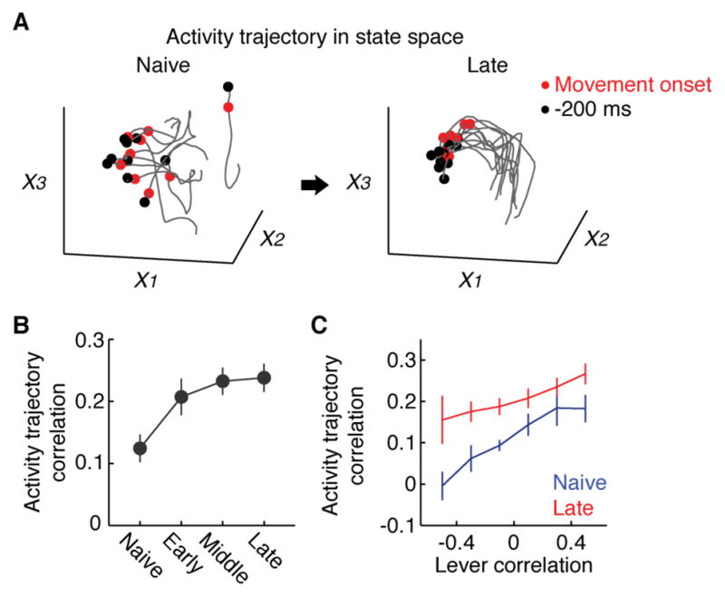
(A) Example of neural trajectories from 10 randomly selected trials in a 3-dimensional state space where axes correspond to the first three factors from Factor analysis computed individually at naive and late stages. Black and red dots are 200 ms before movement onset and movement onset, respectively.

(B) Mean pair-wise correlations of neural trajectories in the state space defined by the 5 factors from factor analysis over learning (p < 0.01, n = 8 mice, regression, mean ± SEM).

(C) Enhanced reliability in the activity pattern after learning regardless of the changes in movement correlation. For each trial pair at each learning stage, lever trajectory correlations and activity trajectory correlations in state space following Factor analysis were calculated and averaged within each lever correlation bin (p < 0.001, n = 8 mice, Friedman test, mean ± SEM).

Emergence of a secondary activity flow from anterior cortical areas during learning

We next addressed whether motor learning influences the spatial propagation of activity across the cortex. Specifically, the activity timing of anterior areas including M2 strongly shifted towards the beginning of the activity sequence (Figure 2D and E), suggesting that the activity may propagate from these anterior areas with learning. To quantify this effect, we measured phase gradients across individual pixels based on space-frequency singular value decomposition (SVD). The space-frequency SVD analysis identifies an orthogonal set of modes, in each of which the magnitude and phase of the spatial coherence of cortex-wide activity are assigned to individual pixels (STAR Methods). Thus, the spatial gradients of phases indicate the local direction of activity flow (i.e. travelling wave) (Mitra and Bokil, 2008; Prechtl et al., 1997). We focused on the leading mode explaining the highest variance, which was consistent over learning and explained 37.2 ± 1.3 (mean ± SEM) %, 37.0 ± 1.2 %, 36.8 ± 2.5 % and 38.6 ± 2.1 % of total variance at the respective learning stages (Figure 4A, top row). At the naive stage, the activity propagated from RSC in a radial direction (Figure 4A, middle and bottom rows). However, at the later stages of learning, an additional activity stream emerged that flowed from M2 to M1/S1 (Figure 4A, middle and bottom rows). An independent analysis based on T_half-max of mean activity in each pixel confirmed these findings (Figure S6).

Figure 4. Emergence of a secondary activity flow from anterior cortical areas.

(A) Magnitude (top row) and phase (middle row) of the spatial coherence of activity of the leading mode identified by space-frequency singular value decomposition (SVD) analysis at each learning stage. Phase gradients (from blue to red) indicate the direction of travelling waves. Bottom row, direction of the phase gradients. Arrows and lines indicate the direction and relative speed of activity propagation within each stage, respectively.

(B) Top, matrix of median Granger causality at each learning stage. Direction of causality is indicated by “from” (blue modules) and “to” (yellow modules). Cortical modules were sorted in the antero (A)-posterior (P) direction (names of modules listed in the blue and yellow boxes). Leftmost column in each matrix is causality from M2 to the rest of the cortex. Only causality with p < 0.01 was included after correction for multiple comparisons by false discovery rate. Bottom, spatial map of causality from M2 (open circles) to other brain areas at each learning stage. Line width reflects the magnitude of causality.

Next, in order to test whether the activity of certain areas predict the activity in other areas on a moment-by-moment basis, we carried out the Granger causality analysis, which identifies directed functional connectivity between brain areas (Barnett and Seth, 2014). This analysis revealed that there was little predictive relationship between modules during the naive stage. With learning, however, M2 rather uniquely acquired a predictive role about the activity of many other brain areas (Figure 4B). Importantly, when we shuffled trials within each session independently for each module, the predictive role of M2 was abolished (Figure S6), indicating that M2’s causality cannot simply be explained by its increase in the speed of activation (Figure 2D). Rather, M2’s predictive role revealed by the Granger causality analysis depends on the trial-by-trial co-variation of activity timing across modules. These results suggest that motor learning strongly modulates the direction of information flow across the cortex and that M2 becomes more influential on the activity of the rest of the cortex.

Impact of M2 inactivation on cortical network dynamics

The Granger causality analysis implies that M2, one of the movement-controlling regions in the brain, gradually exerted stronger influences on the rest of the cortical activity during learning (Figure 4B). To directly test this notion, next we inactivated M2 with muscimol, a GABA receptor agonist, after 2 weeks of behavioral training and monitored the activity of the rest of the cortex (n = 7 mice, Figure 5A, C and D). Muscimol spread was largely restricted to M2 (Figure S7). Inactivation of M2 led to a large impairment in behavior with a significant increase in missed trials (correct rate: 97.2 ± 0.6 % for vehicle and 62.4 ± 8.3 % for muscimol, p < 0.001, Figure 5B). Importantly, M2 inactivation largely eliminated the stereotypy of movements, a hallmark of skill learning (movement correlation: p < 0.05, one-tailed bootstrap, Figure 5B, see Figure S7 for other behavioral parameters). This behavioral impairment was accompanied by a delay in the activity of the majority of cortical modules (Figure 5E and F). Furthermore, the trial-by-trial sequential activity of cortical modules was temporally expanded with M2 inactivation (Figure 5G), indicating that the learning-induced temporal compression of the sequential cortical activity was at least partially dependent on M2. Moreover, the variability of activity trajectory increased (Figure 5H). Thus, M2 inactivation after learning reversed the learning-related changes in the macro-scale activity and the improvement of behavioral performance. These results are consistent with the Granger causality analysis and support the notion that M2 acquires a leading role in the macro-scale activity sequence after learning.

Figure 5. Impact of inactivation of M2 on network dynamics.

(A) Left, schematic of the experiment. Right, muscimol injection sites indicated by the pink arrows, M2 modules and directed functional connectivity from M2 measured by Granger causality analysis.

(B) Effect of module inactivation on behavioral performance. Left, correct rate (97.2 ± 0.6 % for vehicle, 62.4 ± 8.3 % for muscimol, ***p < 0.001, n = 7 mice, one-tailed bootstrap, mean ± SEM). Right, movement correlation (*p < 0.05, n = 7 mice, one-tailed bootstrap, mean ± SEM).

(C) Example peri-movement activity over 1 s with vehicle or muscimol injection in M2 (66.67 ms/image).

(D) Mean activity change with M2 inactivation compared to vehicle (n.s. for all cortical modules, p > 0.05, n = 7 mice, one-tailed bootstrap, mean ± SEM).

(E) Mean T_half-max in cortical modules with vehicle or muscimol injection in M2 (***p < 0.001, **p < 0.01, *p < 0.05, one-tailed bootstrap, corrected for multiple comparisons by false discovery rate, n = 7 mice, mean ± SEM).

(F) Temporal spread of sequential activity with vehicle or muscimol injection in M2.

(G) Temporal spread of trial-by-trial sequential activity with vehicle or muscimol injection in M2 (*p < 0.05, n = 7 mice, one-tailed bootstrap, mean ± SEM).

(H) Mean pair-wise correlations of neural trajectories in the state space defined by the 5 factors from factor analysis with vehicle or muscimol injection in M2 (***p < 0.001, n = 7 mice, one-tailed bootstrap, mean ± SEM).

Impact of RSC inactivation on cortical network dynamics

Next, since pRSC was consistently one of the first nodes of the activity sequence throughout learning (Figure 2E), we tested the effect of pRSC inactivation after 2 weeks of training (n = 6 mice, Figure 6A, C and D). Unlike M2 inactivation, the behavioral performance was minimally affected by pRSC inactivation (correct rate: 96.2 ± 1.3 % for vehicle control and 83.8 ± 6.6 % for muscimol, p < 0.05; movement correlation: n.s., p = 0.19, one-tailed bootstrap, Figures 6B and S7). Moreover, the activity speed, temporal spread of the sequential activity, and activity trajectory correlations were unaffected (Figure 6E–H). These limited effects of pRSC inactivation are consistent with the general lack of significant Granger causality from pRSC to other brain areas throughout learning (Figure 4B). Together, these results highlight the distinct contributions of M2 and pRSC to cortical dynamics and support the importance of M2 to coordinate the cortex-wide activity during motor learning.

Figure 6. Impact of inactivation of pRSC on network dynamics.

(A) Left, schematic of the experiment. Right, muscimol injection sites indicated by the pink arrows, pRSC modules and directed functional connectivity from pRSC measured by Granger causality analysis.

(B) Effect of module inactivation on behavioral performance. Left, correct rate (96.2 ± 1.3 % for vehicle, 83.8 ± 6.6 % for muscimol, *p < 0.05, n = 6 mice, one-tailed bootstrap, mean ± SEM). Right, movement correlation (n.s., p = 0.19, n = 6 mice, one-tailed bootstrap, mean ± SEM).

(C) Example peri-movement activity over 1 s with vehicle or muscimol injection in pRSC (66.67 ms/image).

(D) Mean activity change with pRSC inactivation compared to vehicle (n.s. for all cortical modules, p > 0.05, n = 6 mice, one-tailed bootstrap, mean ± SEM).

(E) Mean T_half-max in cortical modules with vehicle or muscimol injection in pRSC (n.s. for all cortical modules, p > 0.05, n = 6 mice, one-tailed bootstrap, mean ± SEM).

(F) Temporal spread of sequential activity with vehicle or muscimol injection in pRSC.

(G) Temporal spread of trial-by-trial sequential activity with vehicle or muscimol injection in pRSC n.s., p = 0.43, n = 6 mice, one-tailed bootstrap, mean ± SEM).

(H) Mean pair-wise correlations of neural trajectories in the state space defined by the 5 factors from factor analysis with vehicle or muscimol injection in pRSC (n.s., p = 0.36, n = 6 mice, one-tailed bootstrap, mean ± SEM).

Learning-dependency of the observed changes in the cortex-wide dynamics

To test whether the observed changes in the cortex-wide activity were due to learning, we performed an additional experiment in which we imaged cortex-wide activity over weeks in mice that were randomly given rewards irrespectively of lever presses (n = 12 mice, Figure 7A). Under this condition, mice demonstrated only a modest increase in movement stereotypy (within session: p < 0.05; across sessions: p < 0.05, Kruskal-Wallis test, Figure 7B) and failed to reach the level observed in the trained mice (comparison between trained and no-task mice: within session: p < 0.05; across sessions: p < 0.05, one-tailed bootstrap). Thus, these no-task mice showed only a limited level of motor learning. In these mice, both the activity amplitude and speed in each cortical module did not increase (p > 0.05 in all modules, regression, Figure 7C and D). Accordingly, sequential activity across cortical modules did not compress in time (p = 0.56, regression, Figure 7E) and variability of cortex-wide activity showed only a modest decrease (p < 0.01, regression, Figure 7F, compare with Figure 3B). Lastly, Granger causality analysis showed only a minor and slow causality increase from M2 to some of the cortical areas (Figure 7G), paralleling the moderate and slow increase in movement stereotypy. These results suggest that the observed changes in the macro-scale activity dynamics in the task mice are learning-dependent.

Figure 7. Analysis of no-task mice.

(A) Experimental setup. In each trial, the cue period varied randomly between 2 to 5 s, which was followed by reward delivery without the requirement of lever-press. Spontaneous lever movements were continuously monitored.

(B) Left, correlation matrix of the lever trajectory in individual trials. Middle, trial-by-trial correlations of the lever trajectory within each session, corresponding to the central diagonal in the matrix on left (p < 0.05, n = 12 mice, Kruskal-Wallis test, mean ± SEM). Right, trial-by-trial correlations of the lever trajectory across adjacent sessions (p < 0.05, n = 12 mice, Kruskal-Wallis test, mean ± SEM). Unlike the task condition, lever movement stereotypy only mildly increased, indicating a much lower level of motor skill learning in these no-task mice.

(C) Amplitude of movement-related activity at each stage of no-task mice, measured by mean Δf/f between 0 ms and +800 ms relative to the movement onset (n.s. for all cortical modules, p > 0.05, n = 12 mice, regression, mean ± SEM). Since aS1BC were not commonly identified across the no-task mice, these modules were not considered.

(D) T_half-max of 14 cortical modules at each stage (n.s. for all cortical modules, p > 0.05, n = 12 mice, regression, mean ± SEM). Naive, session 1; Early, sessions 3, 5 and 7; Middle, sessions 11, 13 and 15; Late, sessions 16–18.

(E) No temporal compression of sequential activity over no-task sessions (p = 0.56, n = 12 mice, regression, mean ± SEM).

(F)Top, mean pair-wise correlations of neural trajectories in the state space defined by the 5 factors from factor analysis over control sessions (p < 0.01, n = 12 mice, regression, mean ± SEM). Note that although there is a small increase in the activity trajectory correlations over sessions, they are generally lower than the task mice.

(G) Top, matrix of median Granger causality at each stage of no-task mice. Bottom, spatial map of causality from M2 (open circles) to other brain areas at each control stage. Note that the causality from M2 is weaker and its emergence is slower than the task mice.

Population dynamics of M2 neurons during learning revealed by two-photon calcium imaging

The results so far have identified M2 as an important organizer of the cortex-wide network during learning. To explore the cellular basis underlying the change, we performed longitudinal two-photon calcium imaging to examine the dynamics of M2 microcircuits at cellular resolution during learning. We examined M2 excitatory neurons in L2/3 and L5 using CaMKIIα-tTA × tetO-GCaMP6s transgenic mice (Wekselblatt et al., 2016) (n = 171 ± 23 neurons per mouse in 9 mice for L2/3, n = 240 ± 24 neurons per mouse in 7 mice for L5, Figure 8A and B). The same neurons were imaged over the course of learning (2 weeks). We inferred the spike rate from calcium imaging data using the spike-triggered mixture (STM) model (Theis et al., 2016). During learning, the ensemble activity during movement shifted earlier in time especially in L5 (p = 0.64 for L2/3, Kolmogorov-Smirnov test, Figure 8C; p < 0.001 for L5, Kolmogorov-Smirnov test, Figure 8D), and the neurons exhibiting pre-movement activity increased in L5 (1.7 ± 0.6 % for naive and 9.9 ± 2.5 % for expert out of all neurons, p < 0.001, one-tailed bootstrap; 10.4 ± 1.8 % for naive and 18.9 ± 3.1 % for expert out of movement-modulated neurons, p < 0.01, one-tailed bootstrap). In addition, trial-by-trial correlations of movement-related activity within and across sessions increased in both layers (p < 0.05 for L2/3, regression, Figure 8E and G; p < 0.001 for L5, regression, Figure 8F and H), suggesting that reliable and reproducible activity patterns emerged with learning, similar to what has been shown in M1 (Peters et al. 2014). This decrease in variability, however, was not solely due to the decrease in movement variability. When calculating the activity correlation between similar and dissimilar lever movements, we found higher correlation in expert animals regardless of movement similarity (Figure 8I and J, magenta and grey lines). These increases in the speed and consistency of movement-related activity of M2 microcircuit resonate with the results from wide-field imaging.

Figure 8. Two-photon calcium imaging of M2 excitatory neurons in L2/3 and L5.

(A) Left, experimental setup. Right, two-photon images of GCaMP6s-expressing neurons in L2/3 and L5.

(B) Activity of example neurons over learning.

(C) Cumulative probability distribution of activity onsets of movement-modulated neurons in L2/3 (n.s., p = 0.64, n = 231 neurons for naive and n = 640 neurons for expert, Kolmogorov-Smirnov test). Naive and expert are sessions 1–2 and sessions 11–14, respectively.

(D) Same as (C) for L5 (p < 0.001, n = 264 neurons for naive and n = 726 neurons for expert, Kolmogorov-Smirnov test).

(E) Trial-by-trial population activity correlation of movement-modulated neurons in L2/3 in each session (p < 0.05, n = 9 mice, regression, mean ± SEM).

(F) Same as (E) for L5 (p < 0.001 n = 7 mice, regression, mean ± SEM).

(G) Trial-by-trial population activity correlation of neurons that are movement-modulated in at least one session in L2/3 across sessions.

(H) Same as (G) for L5.

(I) Trial-by-trial population activity correlation in L2/3 as a function of trial-by-trial movement correlation within and across naive and expert stages (p < 0.001, n = 9 mice, Friedman test, mean ± SEM).

(J) Same as (I) for L5 (p < 0.001 n = 7 mice, Friedman test, mean ± SEM).

(K) Fraction of movement-modulated neurons over learning for L2/3 (p < 0.001, n = 9 mice, regression, mean ± SEM).

(L) Same as (K) for L5 (p < 0.001, n = 7 mice, regression, mean ± SEM).

These changes in population activity were accompanied by heterogeneous changes of individual neurons, resulting in a turnover of the identity of movement-related neurons throughout learning. Overall, the fractions of movement-modulated neurons increased in both layers during learning (p < 0.001 for L2/3, regression, Figure 8K; p < 0.001 for L5, regression, Figure 8L, STAR Methods), with increases in both movement-activated and movement-suppressed neurons (Figure S8). Thus, neurons in M2 are increasingly recruited for the learned movement. Through these turnovers, however, the population of movement-modulated neurons gradually stabilized (Figure S8). In line with these turnovers of movement-modulated neurons, the population activity during individual movements showed low correlations between naive and expert stages (Figure 8G and H). Activity correlations were consistently low even when we compared movements with similar kinematics in naive and expert animals (Figure 8I and J, blue lines), indicating the emergence of a novel activity-movement relationship. These results at cellular resolution uncover dynamic changes of neuronal population activity in M2 underlying its evolving control over the cortex-wide activity during learning.

DISCUSSION

Our wide-field calcium imaging provides an unbiased, macroscopic view of the activity dynamics across the dorsal cortex. This approach afforded us sufficient temporal resolution and signal-to-noise ratio to uncover novel emergent properties of cortex-wide dynamics with single trial analyses. Distinct brain areas could be identified based solely on the correlation structures of activity of individual pixels. For many areas in the rodent cortex, the precise locations and the borders between areas are often poorly defined. Wide-field calcium imaging with the ICA-based pixel grouping provides an efficient way to functionally define cortical modules in individual mice. It is also likely that future imaging performed while mice are in richer behavioral contexts and larger repertoire of sensory stimuli would identify additional cortical modules and perhaps subdivide some of the modules defined in this study. Intriguingly, some modules were identified across hemispheres, while other modules were separated in each hemisphere. In general, primary areas such as M1 and S1 were identified separately in each hemisphere, while higher and associational areas such as M2, PPC and RSC were identified as bilateral modules. This observation may support the view that bilateral interactions are important for the functions of higher brain areas (Li et al., 2016), resulting in more correlated macro-scale activity in both hemispheres of these higher areas.

We found that the learning of the lever press task involved distributed activation of most of the cortex, forming a macroscopic sequential activity. With learning, this macroscopic sequence of activity during movement execution became more temporally compressed and reproducible, suggesting a more efficient and reliable signal transmission across cortical modules. A recent study described a macroscopic activity sequence in a context-dependent decision making task (Siegel et al., 2015). Our results suggest that such an activity sequence evolves as a function of learning. It is important to note that the temporal compression of cortical activity flow is not a result of an enhanced speed of the movement. The temporally compressed and reliable cortical activity sequence may evolve with learning to more effectively trigger subcortical movement machinery.

Our unbiased monitoring of macroscopic dynamics revealed a surprising role acquired by M2. (We note that our M2 overlaps with areas that are sometimes referred to as frontal association area and ALM. The available data do not distinguish whether these areas are actually the same area with different names, or overlapping but distinct.) With learning, a novel activity stream emanated from M2 and flowed to the rest of the cortex, and the activity of M2 acquired a predictive role of the activity of the other modules on a moment-by-moment basis. This is as if M2, after learning, acts as a conductor to orchestrate the network activity of the rest of the cortex. We note that this correlation-based Granger causality analysis does not address whether the causality is due to direct connectivity. We also note that it is unlikely that M2 is the only area that drives the behavior. Nevertheless, consistent with the increase of the causality from M2 to other modules, our inactivation experiments showed that M2 is necessary for the rapid induction and reliable execution of macroscopic sequential activity acquired with learning. Concurrently, learning induced novel and stable movement-related populations in M2, resonating with another recent study observing the Arc promoter activity during motor learning (Cao et al., 2015). Premotor cortex such as M2 is generally considered to be important for movement planning and preparation (Churchland et al., 2006; Godschalk et al., 1985; Guo et al., 2014; Murakami et al., 2014; Weinrich and Wise, 1982), presumably through their reciprocal connections with M1 and direct subcortical projections. These previous recordings were obtained from well-trained animals. Our results suggest that the role of M2 in movement preparation may evolve with learning.

This study lends support to the view that the brain has multiple modes of operation to generate a given movement. Our recent study demonstrated that there is substantial degeneracy between microcircuit activity of M1 and movement kinematics and that motor learning shapes the relationship between M1 activity and movement (Peters et al., 2014). Our current study extends this notion to macro-scale activity across cortical areas. Specifically, there appear to be two different modes of movement execution; M2-independent and M2-dependent, the latter of which may be a hallmark of learned movements. Such recruitment of the frontal cortex during learning is consistent with the notion that cognitive control is critical during skill acquisition (Floyer-Lea and Matthews, 2004; Sakai et al., 1998; Toni et al., 1998), and is reminiscent of our recent study demonstrating that learning recruits top-down control in sensory processing (Makino and Komiyama, 2015). We propose that the cortical activity flow is fundamentally flexible, and a unique and novel activity flow may emerge specifically for each learned behavior.

STAR METHODS

CONTACT FOR REAGENT AND RESOURCE SHARING

Further information and requests for resources and reagents should be directed to and will be fulfilled by the lead contact Takaki Komiyama (tkomiyama@ucsd.edu).

EXPERIMENTAL MODEL AND SUBJECT DETAILS

All procedures were in accordance with the Institutional Animal Care and Use Committee at University of California, San Diego. Mice were obtained from The Jackson Laboratory (Thy1-GCaMP6s: C57BL/6J-Tg(Thy1-GCaMP6s)GP4.3Dkim/J [JAX 024275]; Thy1-GFP: B6;CBA-Tg(Thy1-EGFP)SJrs/NdivJ [JAX 011070]; CaMKIIα-tTA: B6;CBA-Tg(Camk2a-tTA)1Mmay/J [JAX 003010]; tetO-GCaMP6s: B6;DBA-Tg(tetO-GCaMP6s)2Niell/J [JAX 024742]). Mice were typically group housed with a reversed light cycle (12h-12h) in standard plastic disposable cages. Experiments were performed during the dark period. Both male and female healthy adult mice were used and randomly assigned to each experimental group. Mice had no prior history of experimental procedures that could affect the results.

METHOD DETAILS

Surgery

For wide-field calcium imaging

Adult mice (between 6 weeks and 4 months old) were anesthetized with 1–2 % isoflurane and a circular piece of scalp was removed. After cleaning the underlying bone using a razor blade, a custom-built head-post was implanted to the exposed skull (~0.5 mm posterior to lambda) with cyanoacrylate glue and cemented with dental acrylic (Lang Dental). The skull was protected by cyanoacrylate glue applied several times over ~1 hour. Heat shrink tube (diameter: 2 cm) cut to ~5 mm was then glued to the circumference of the skull, which minimized the entry of the excitation light to the eyes during imaging. General analgesia (buprenorphine, 0.1 mg/kg body weight) was subcutaneously injected and mice were monitored until they recovered from anesthesia. Any mice that had poor optical access to the cortex due to infection, poor surgery etc. were excluded.

For two-photon calcium imaging

Adult mice (between 6 weeks and 4 months old) were anesthetized with 1–2 % isoflurane. Dexamethasone (2 mg/kg) and baytril (10 mg/kg) were injected subcutaneously. A custom-made head plate was attached to the skull with dental cement and craniotomy (1.5 mm diameter) was performed over the right M2 module. A chronic imaging window was implanted consisting of a glass plug glued on to a larger glass base (Komiyama et al., 2010). Buprenorphine (0.1 mg/kg body weight) was given subcutaneously at the end of surgery.

Behavior

For wide-field calcium imaging

After recovering from surgery, mice were water restricted to 1 ml per day. After a few weeks of water restriction, mice were trained to perform the lever-press task one session per day over weeks. The behavior setup, which was controlled by software (Dispatcher, Z. Mainen and C. Brody) running on MATLAB with a real-time system (RTLinux), has been described previously (Peters et al., 2014). Briefly, a 6 kHz tone (up to 10 s) marked a cue period, during which a successful lever press was rewarded with water (~10 μl per trial) paired with a 500 ms, 12 kHz tone, and an inter-trial interval (variable duration of 8–12 s) followed. A successful lever press was defined as crossing of two thresholds (~1.5 mm and ~3 mm below the resting position) within 200 ms. The 3 mm threshold defined the displacement required for a successful press and the 1.5 mm threshold prevented the mouse from holding the lever near the lower threshold. Failure to press the lever passing the two thresholds during the cue period triggered a loud white noise and an inter-trial interval. Lever presses during inter-trial intervals were neither rewarded nor punished. Each training session was terminated when the animal reached ~80 successful trials or when it stopped performing. One mouse failed to learn the task and was excluded from analyses. For the no-task experiment, the task structure was similar except that reward (~10 μl water per trail) was delivered after variable duration of a cue (2–5 s) in each trial without the requirement of lever-press. Each no-task session contained 80 trials. The lever position was continuously monitored through a piezoelectric flexible force transducer using LabVIEW (National Instruments) and licking was detected by a touch detector (Slotnick, 2009) or an infrared lickometer (Island Motion Co.). The lever position and licking were constantly recorded by Ephus in MATLAB (MathWorks).

For two-photon calcium imaging

After recovery from surgery, mice were water restricted at 1 ml per day. After 14 days of water restriction, mice were trained to perform the lever-press task one session per day for 14 days with simultaneous two-photon imaging. The behavior setup was controlled by an open-source, Arduino-based behavioral control software (Bpod, SanWorks) and Arduino boards (Arduino). The lever-press task was designed similarly as described in the above section except for the duration of auditory cue (30 s in the first session and 10 s in later sessions) and inter-trial interval (variable duration of 10–15 s). Mice performed 120 ± 2 (mean ± SEM) trials per session.

Movement analysis

Lever traces were first down-sampled from 10 kHz to 1 kHz and then filtered (4 pole 10 Hz low-pass Butterworth). The velocity of the lever was then determined by smoothing the difference of consecutive points with a moving average window of 5 ms. The envelope of the velocity was then extracted using a Hilbert transform, and movement bouts were defined by the envelope crossing a threshold (4.9 mm per second). Bouts separated by less than 200 ms were considered continuous. The beginning and end of each movement bout were identified as previously described (Peters et al., 2014). Briefly, movement was detected by a velocity threshold (4.9 mm per second), and the onset and offset of movement bouts were identified by the lever position leaving or entering the resting period respectively. The trials in which animals were moving the lever at the onset of cue were excluded. Lever traces on different trials were collected from the onset of each intended movement to 800 ms after the onset of movement, which was approximately the duration of intended movements for all animals over all sessions (610.7 ± 72.8 ms, mean ± SEM). The intended movement was defined as the movement initiated between cue onset and reward. In the no-task mice, movements selected for activity analysis were those initiated after the cue onset and the time between passing the first and second thresholds was less than 200 ms during the cue. Similarity of lever trajectories across trials was computed by Pearson correlation (Figures 1C, 2H, 3C, 5B, 6B, 7B, 8H and J). Changes in lever correlations in task and no-task mice were compared by computing a slope of a linear fit for individual mice.

Data acquisition by wide-field calcium imaging

Wide-field calcium imaging was performed using a commercial fluorescence microscope (Axio Zoom.V16, Zeiss, objective lens (1×, 0.25 NA)) and a CMOS camera (ORCA-Flash4.0 V2, Hamamatsu) through the intact skull. Images were acquired using HCImage Live (Hamamatsu) at 29.98 Hz, 512 × 512 pixels (field of view: 11 mm × 11 mm, binning: 4, 16 bit) every other session of behavioral training. Each session consisted of several trial blocks, each of which contained 9000 frames corresponding to 5 min. For some mice, every other block was imaged to minimize potential photobleaching. Imaging and behavioral data were acquired simultaneously and aligned offline based on a synchronization signal.

Two-photon calcium imaging

Imaging was conducted with a commercial two-photon microscope (MOM scope, Sutter Instruments, retrofitted with a resonant galvanometer-based scanning system from Thorlabs), 16× objective (Nikon) and 925 nm excitation light (Ti-Sapphire laser, NewPort) controlled by ScanImage (Vidrio Technologies). Images were recorded at approximately 28 Hz continuously, with a field view of 472 × 508 μm with 512 × 512 pixels. Frame times were recorded and synchronized with behavioral recording by Ephus. Slow drifts in imaging field were manually corrected using reference images. Imaging was performed approximately 250 μm deep from dura for L2/3 and 500 μm for L5. 4 mice were imaged for L2/3 only, 2 mice for L5 only, 5 mice for both (alternating between L2/3 and L5 each day).

Electroencephalography

Thy1-GCaMP6s mice were prepared as described in the above section. A transparent graphene electrode array (Kuzum et al., 2014) with 4 × 4 channels (1.8 × 1.8 mm for the whole array and 180 × 180 μm for each channel, data recorded by channels with impedance < 1 kΩ were used for analysis) was place over the right S1HL (1.8 mm lateral and 1 mm posterior to bregma) and electrical gel (Parker Laboratories) was applied locally to ensure good contact. A stainless-steel screw (F000CE156, J.I. Morris) was implanted over cerebellum as reference. After the mouse recovered from anesthesia, EEG recording and wide-field calcium imaging were performed simultaneously. Electrical signal was amplified and recorded using RHD2000 at 10 kHz (Figure S2E–G).

Multi-unit recording

Thy1-GCaMP6s mice were anesthetized with 1–2% isoflurane and a circular piece of scalp was removed to expose the skull. After cleaning the soft tissue on top of the bone using a surgical blade, a custom-built head-bar was implanted to the exposed skull over the cerebellum (~1 mm posterior to lambda) with cyanoacrylate glue and cemented with dental acrylic (Lang Dental). The dorsal surface of the skull was left uncovered. A craniotomy (~1mm in diameter) was made over the frontal cortex. Another small craniotomy was made posterior and lateral to the recording site and a ground wire was placed under dura. Electrophysiological recording was performed with a tungsten electrode (FHC) with impedance ~250 kΩ measured at 1 kHz. Electrode was held by a custom-made electrode holder attached to a micromanipulator (MP-285, Sutter). After the mouse recovered from anesthesia, the electrode was inserted into the frontal cortex at 30° to the horizontal plane. Distance traveled was recorded and used to estimate the location of electrode tip. Electrical signal was amplified and recorded using RHD2000 Evaluation System (Intan) at 20 kHz with simultaneous wide-field calcium imaging (Figure S2H–J).

Electrophysiology and EEG data analysis

Calcium event detection for wide-field imaging

Calcium traces were extracted by taking the mean Δf/f (Δf/f was calculated as described in section Wide-field calcium imaging analysis) within ROIs. The first derivative (velocity) of the smoothed Δf/f trace (loess, 1 s) was calculated and the inactivate portion was defined as the periods when the velocity was within the standard deviation of the whole velocity trace. Events were defined if the velocity trace crossed the standard deviation of the inactive portion of the velocity trace. This method detected sharp rises in Δf/f. For each event, the onset time was first estimated as the time when the velocity exceeded the velocity criterion, and the offset time was estimated as the time when the velocity dropped below zero for the first time after the onset. The onset time was further refined as follows. For each event, the baseline Δf/f was defined as the value at the first time point when the velocity was above zero before the offset time, and Δf/f noise level was defined as the mean of the absolute difference between the raw and smoothed Δf/f traces. The onset was refined as the last time point before the offset time when the Δf/f value is within noise level from the baseline Δf/f. The offset time was further refined as the time of the highest Δf/f value within five frames before and after the initial estimate. Calcium events with a preceding inactive period of at least 1 s were selected for EEG and MU data analysis (Figure S2G, I and J). For EEG experiments, an ROI around the right S1HL area under the transparent electrode and another ROI with the similar size on the left frontal area were drawn manually. For MU recording, a 1-mm circle centered at estimated electrode tip was used as ROI.

MU data analysis

Recorded signal was first band-pass filtered by 500–10000 Hz. A threshold was determined as 3 times the median absolute deviation of the whole recording session below the mean. Signal deflections that exceeded the threshold were registered as spikes. Spike trains from −1 to +1 s relative to calcium event onset were aligned and firing rate was calculated using a 50-ms moving window with 10-ms steps. To determine the onset of MU activity, activity during −1 to −0.5 s was pooled as baseline. The firing rates at each data point were compared to the baseline by bootstrap (10,000 repetitions) and significantly modulated data points were identified (p < 0.01). We defined significantly modulated periods as those with at least 4 consecutive significant points (Figure S2H–J).

EEG data analysis

EEG traces were first filtered (2-pole 50 Hz low-pass Butterworth) and then down-sampled to 1 kHz. EEG traces from −1 to +1 s relative to calcium event onset were aligned. The aligned EEG traces were directly used to detect the modulation of EEG activity by bootstrapping as described in the above section (Figure S2E–G).

pRSC/M2 inactivation

Following 15 sessions of behavioral training, muscimol hydrobromide (5 μg/μl, Sigma) was injected in pRSC (bilateral injections at 0.3 mm lateral and 3.2 mm posterior to bregma at the depths of 300 μm and 600 μm from the brain surface) or M2 (bilateral injections at 1.0 mm lateral and 2.6 mm anterior to bregma at the depths of 300 μm and 600 μm from the brain surface) under anesthesia with 1–1.5% isoflurane with a beveled pipette (~20 μm tip in diameter) through a small (~0.5 mm in diameter) craniotomy (~10–30 nl at each site at the speed of ~20 nl/min). Pipettes were left in the brain for additional ~4 min after each injection. As a control, vehicle (saline) was similarly injected. Following injections, mice recovered from anesthesia in their home cage for 1–1.5 hours before behavioral testing and imaging. The same procedure was repeated 3 times for muscimol and vehicle injections (one muscimol or vehicle session per day, total of 6 sessions) and results were averaged. In two cases of M2 inactivation, mice were obviously impaired with movement and failed to lick during task and these sessions were excluded. In two other animals, the S1/M1FL module was not identified from PCA/ICA, possibly due to muscimol spread into this area, and these sessions were also excluded from data analysis.

Two-photon calcium imaging during M2 inactivation

To determine the effectiveness of muscimol inactivation (Figure S7A), baseline activity level of M2 excitatory neurons from three awake animals (cross between CaMKIIα-tTA and tetO-GCaMP6s) was recorded under a two-photon microscope through a chronic glass window. After 10-min baseline recording, muscimol injection (~20 nl at the depths of 300 μm and 600 μm at the speed of ~20 nl/min) was performed as described in the above section, through a small hole drilled through the glass window, ~1 mm from the imaging site. After injection, mice recovered from anesthesia in their home cage for 1–1.5 hours before another 10-min two-photon recording.

Fluorescein injection

To approximate the spread of muscimol during inactivation experiments (Figure S7B), a low-molecular-weight fluorescein (disodium salt, MW = 412, Fisher, (Siniscalchi et al., 2016)) was injected in the left M2 of two wild-type mice following the same procedure of muscimol injection. Fluorescein was at the same concentration and volume used for muscimol injection (~25 mM, ~20 nl at each site at the speed of ~20 nl/min). 1 hr after injection, animals were anesthetized (ketamine/xylazine, 150 mg/kg, 12 mg/kg body weight) and perfused transcardially with 1× PBS. The brain was immediately sectioned at 200 μm with a vibratome (VT1000 S, Leica) and brain slices were imaged using a fluorescence microscope (Axio Zoom V16, Zeiss, objective lens 1×, 0.25 NA). All slices were imaged at the same parameters including the exposure time and excitation power. Images of brain slices were registered with the coronal mouse brain atlas from the Allen Brain Institute to estimate the AP location and structures. The total brightness of fluorescein of each brain slice was measured in MATLAB as follows. For each slice, a baseline ROI was drawn manually in the hemisphere without fluorescein injection at the location corresponding to the fluorescein signal. The signal ROI was defined as the continuous pixels whose brightness exceeds the mean +5 × SD of the baseline ROI. The same ROI was further applied to the other hemisphere as the background ROI to ensure that the location and number of selected pixels were same between two hemispheres. The total brightness of each brain slice was calculated by subtracting the integrated brightness of pixels within the background ROI from the signal ROI.

Inhibition of synaptic transmission with NBQX/CPP

Awake condition

Five animals (Thy1-GCaMP6s) under slight anesthesia (0.8-0.5 % isoflurane) were injected with a mixture of NBQX (2–4 mM, Tocris) and CPP (1–2 mM, Tocris) in left S1HL (1.8 mm lateral and 1.0 mm posterior to bregma at the depths of 300 μm and 600 μm from the brain surface) with a beveled pipette (~20 μm tip in diameter) through a small (~0.5 mm in diameter) craniotomy (~100–200 nl at each site at the speed of ~20 nl/min). Pipettes were left in the brain for additional ~4 min after each injection. As a control, vehicle (saline) was similarly injected. Following injections, mice recovered from anesthesia in their home cage for ~15–20 min before behavioral testing and imaging (Figure S2C). We avoided M2 as the injection site since blocking synaptic transmission in this area could result in a complicated effect, such as a change in movement, and this potential confounding factor would make the interpretation difficult.

Anesthetized condition

Three mice were anesthetized with an intraperitoneal injection of a mixture of ketamine (100 mg/kg body weight) and xylazine (8 mg/kg body weight). ~15 min after ketamine/xylazine injection, a foot shock (0.5 mA, 500 ms-long) was delivered to the right hind limb every 20 s through two wires attached to a stimulus isolator (A.M.P.I) while the cortex was imaged. A control session (14–15 trials, no injection) was followed by an inhibition session (14–15 trials) in which a mixture of glutamate receptor antagonists, NBQX (2 mM, Tocris) and CPP (1 mM, Tocris), was injected into the left S1HL as above. The inhibition session was carried out ~15 min after NBQX/CPP injection. The anesthesia depth was constantly monitored by toe pinch and eye poke, and an additional dose was supplied when necessary (Figure S2D).

Wide-field calcium imaging analysis

Pre-processing

All analyses were performed using custom codes in MATLAB (MathWorks). 512 × 512 pixel images were first down-sampled to 128 × 128 pixels. To obtain Δf/f time series for each pixel, time-varying baseline fluorescence (f) was estimated for a given time point as the 10th percentile value over 30 seconds around it. For the beginning and end of each imaging block, the following and preceding 15-second window was used to determine the baseline, respectively.

Principal/independent component analysis

Δf/f time series for each pixel was aligned to movement data and the frames during the peri-movement epoch (−200 ms to +800 ms relative to the movement onset) were concatenated across all trials from all sessions for each animal to perform principal component analysis (PCA). In PCA, pixels were treated as variables and the Δf/f time series for individual pixels were treated as observations. Here, principal components corresponded to uncorrelated but not necessarily independent spatial modes. The first 40 principal components that explained 94.42 ± 0.75 (mean ± SEM) % of the total variance were subsequently used for independent component analysis (ICA). ICA is a data transformation method that finds independent sources of activity in recorded mixtures. The ICA algorithm adopted in the current study was JADER (Cardoso, 1999), which decomposes mixed signals into independent components by minimizing the mutual information (estimated by cross-cumulants) using a series of Givens rotation. The components were considered to be independent when the Givens angle in each rotation was smaller than 7.8 × 10⁻⁹ rads. Forty independent components were extracted by JADER based on the first 40 principal components. Here, independent components were spatial modes forced to be as independent as possible. Most independent components corresponded to known brain structures or a particular type of artifacts due to blood vessels or motion. Independent components corresponding to artifacts were manually identified and excluded, and the remaining independent components were considered as cortical modules and named based on the mouse brain atlas from the Allen Brain Institute (Figure S3A). Images were reconstructed by first calculating the products of weights of the independent components with scores of their time series, and then adding to each pixel the mean value of that pixel from the original movie. The second step was performed because the initial PCA subtracted the mean of each pixel. The resulting reconstructed movie specifically retains the activity of individual cortical modules, while effectively reducing artifacts.

Activity analysis

To identify common cortical modules across mice (Figure S3B and C), cortical modules from 8 mice from the first set of experiments were compared. We randomly selected a mouse and used it as a template. Modules in the template mouse were compared to modules from other mice through spatial correlations. For a given template module, the module with the highest spatial correlation coefficient from another mouse was considered to be a common module between the two mice and the similarity of modules across the two mice was manually confirmed. In the case where multiple template modules identified the same module from another mouse as common, only the one with higher similarity was selected through manual inspection. The template mouse was similarly compared with all the non-template mice, which in the end yielded 16 non-overlapping cortical modules that were commonly identified across all mice in the task experiment. The coordinates for the centers of these 16 modules are: M2: ±1.2 ML, +2.3 AP; left and right S1/M1FL: ±3.2 ML, +1.3 AP; left and right aS1BC: ±3.8 ML, −0.4 AP; left and right M1: ±2.6 ML, −0.4 AP; left and right S1HL: ±1.8 ML, −1.0 AP; left and right pS1BC: ±3.3 ML, −1.6 AP; PPC: ±2.1 ML, −1.8 AP; aRSC: ±0.8 ML, −1.8 AP; pRSC: ±0.9 ML, −3.1 AP; left and right visual cortex: ±3.0 ML, −3.3 AP. For pRSC and M2 inactivation experiments (Figures 5, 6 and S7), pRSC and M2 modules were not considered, respectively. For these experiments, the ICA-based method described above was applied in the control and inactivation sessions, and those modules that matched the template modules were selected via manual inspection. In cases where matching modules were not identified in the ICA method, the corresponding modules from the initial learning experiment from the same animal were used. For the no-task experiment, a similar procedure was followed to the task experiment, which yielded 14 non-overlapping cortical modules that were commonly identified across all mice. For each cortical module, Δf/f time series was computed as the mean of the pixel values within each independent component above a weight threshold of 3.5.

Only correct trials were considered. To analyze the amplitude of movement-related activity (Figures 1F, 5D, 6D and 7C), peri-movement Δf/f of each cortical module in each mouse was trial-averaged and the Δf/f value at −200 ms of the trial-averaged trace was subtracted. The mean of the trial-averaged peri-movement Δf/f between 0 and +800 ms relative to the movement onset was considered as movement-related activity. These values were further binned into 4 different learning stages by taking their mean in each mouse (naive: session 1; early: sessions 3, 5 and 7; middle: sessions 11, 13, 15; late: 3 sessions after the 15th session, which corresponds to sessions with vehicle injection into pRSC). The same bins were used hereafter unless noted otherwise. T_half-max (Figures 2C–H 5E–G, 6E–G, 7D, E and S5) was obtained by subtracting the Δf/f at the movement onset from peri-movement Δf/f and normalizing the resulting trace to the peak value between 0 to +800 ms. The time from the movement onset that corresponds to the normalized Δf/f of 0.5 was then identified as T_half-max. If, in a given module, the sum of single-trial Δf/f or trial-averaged Δf/f during the last 400 ms of the peri-movement epoch was negative, T_half-max was not determined for the single-trial (trials excluded over learning: 9.3 ± 2.4 (mean ± SEM) %) or trial-average (sessions excluded over learning: 1.4 ± 0.5 (mean ± SEM) %) analysis, respectively. Temporal compression of sequential activity (Figures 2G, H, 5G, 6G and 7E) was measured by standard deviation of T_half-max from 16 cortical modules on a trial-by-trial basis and averaged in each mouse. If a trial is composed of negative Δf/f in more than 11 out of 16 modules, the trial (2.7 ± 1.1 (mean ± SEM) % over learning) was excluded from the analysis. The p value for temporal compression with similar levels of lever correlations (Figure 2H) was determined as a probability of obtaining a positive slope with regression after computing the slope in bootstrap resampled data in 1000 permutations.

To visualize system-wide neural trajectories, we used factor analysis with 5 common factors using MATLAB and custom code (Figures 3, 5H, 6H and 7F). Factor analysis was used since it can effectively discard independent variability unique to each module compared to PCA.

For the experiment of inhibiting synaptic transmission (Figure S2C and D), ROIs were manually drawn around the injection site (~1 mm in diameter). Pixels directly over the craniotomy were excluded as craniotomy occasionally occluded fluorescence signal. The shock onset frame was subtracted from all the frames and the mean of trial-averaged Δf/f during 2 s after shock onset was calculated.

For the control experiment testing whether the fluorescence signal was due to calcium (Figure S3D and E), the same independent components as above were applied to raw df images (i.e. without removing artifacts with PCA/ICA) of Thy1-GCaMP6s and Thy1-GFP mice. To analyze the amplitude of fluorescence changes, peri-movement Δf/f of each cortical module in each mouse was trial-averaged and the Δf value at −200 ms of the trial-averaged trace was subtracted. The mean of the trial-averaged peri-movement Δf between 0 and +800 ms relative to the movement onset was considered as movement-related fluorescence changes.

To determine whether the temporal compression of sequential activity reflected changes in behavioral parameters, such as movement speed and lever trajectory correlations, the trial-by-trial temporal activity spread was measured within similar behavioral parameter ranges. For movement speed (Figure 2H), trials were separated into 3 speed bins (lever displacement over 400 ms after movement onset, binned into 3 equal numbers of trials across all movements: 0.0043 to 0.0154 mm/ms; 0.0154 to 0.0203 mm/ms; 0.0203 to 0.0589 mm/ms) at each learning stage. For each speed bin, temporal activity spread was then calculated with standard deviation and normalized to the naive stage. These values were then averaged across speed bins. For lever trajectory correlations (Figure 2H), a template lever trajectory was created by averaging randomly chosen 50 % of trials of the late stage. For each learning stage, trials with lever trajectory correlations of more than 0.6 with the template were analyzed. For the late stage, trials were selected for analysis from the remaining 50% of the trials. Temporal activity spread was then determined in these trials at each learning stage.

To determine whether the enhanced activity reliability after learning was not solely attributable to the increase in lever trajectory correlations (Figure 3C), activity trajectory correlations in state space defined by Factor analysis were computed for different lever correlation bins (−0.6 to −0.4; −0.4 to −0.2; −0.2 to 0; 0 to 0.2; 0.2 to 0.4; 0.4 to 0.6) at the naive and late stages.

Space-frequency singular value decomposition

Space-frequency SVD was performed using Chronux version 2.11 (Figure 4A) (Mitra and Bokil, 2008) (http://chronux.org). Briefly, time series data were created for each pixel by concatenating trial-by-trial Δf/f traces during the peri-movement epoch (−200 ms to +800 ms relative to the movement onset) for each session in each mouse. This rearranged dataset exhibits peaks at a fundamental frequency of 1 Hz and its harmonics when represented in a frequency domain. The time series was centered by subtracting the mean value for each pixel. The power spectrum was obtained from the space-time data through Fourier transforms with 18 Slepian tapers. A space-frequency SVD was then applied to the resulting complex matrix to obtain spatial patterns of coherence for a fixed frequency; in this case the frequency was set to be 1 Hz and other parameters were set as the following (frequency band: between 0.1 and 20 Hz; time-bandwidth product = 10; pad = 0; mode kept = 18. The results were robust to different parameter choices.). The decomposed data provide orthogonal sets of spatial modes representing the spatial distribution of coherence at 1 Hz and phase. Gradients in the phase indicate the direction of travelling waves during the peri-movement epoch. We only focused on the leading spatial mode determined by the highest singular value for our analysis, which accounted for 37.2 ± 1.3 %, 37.0 ± 1.2 %, 36.8 ± 2.5 % and 38.6 ± 2.1 % of total variance at naive, early, middle and late stage, respectively (mean ± SEM). The magnitude and phase of the leading spatial mode were then averaged across mice at each learning stage. The magnitude was binned into 24 equally spaced values for a display purpose. The phase was also binned into 12 equally spaced values but pixels with the lowest 3 magnitude bins were excluded for display. As expected, coherence, calculated by the ratio of the power of the leading mode to the total power, revealed peaks at 1 Hz and its harmonics.

As another measure of activity propagation (Figure S6A), T_half-max was determined in individual pixels on trial-averaged activity traces in each mouse at each learning stage. T_half-max was then averaged across mice and binned into 12 equally spaced values for a display purpose.

Granger causality analysis

Granger causality analysis was performed using the multivariate Granger causality toolbox (Figures 4B, 5A, 6A, 7G and S6B) (Barnett and Seth, 2014). For each cortical module, Δf/f at the time of movement onset was first subtracted from Δf/f time series during the peri-movement epoch in a given trial to meet the covariance stationary precondition (i.e. no change in mean and variance over time). Time series data were then created for each module by concatenating the resulting Δf/f traces for all mice (task: n = 8 mice; no-task: n = 12 mice). Time-domain Granger causality was then calculated from the time series data with the multivariate Granger causality toolbox. This toolbox computes Granger causality based on vector autoregressive modeling. The number of time lags (model order) was estimated by Akaike information criteria with the maximum set to be 20. Ordinary-least-squares was used to compute regression coefficients. Pair-wise conditional causality was then calculated. (i.e. for a given ‘to’ module (‘X’), conditional causality for a ‘from’ module (‘Y’) is the degree to which Y’s past helps predict X, over and above the degree to which X is predicted by the past of X and the other conditioning modules (task: 14 modules; no-task: 12 modules)). Conditional causality values that reached statistical significance (p < 0.01) after false discovery rate multiple comparison correction were kept and others were set to zero, and the median of the causality values across mice was obtained at each learning stage.

Two-photon calcium imaging analysis

Images were first aligned frame-by-frame using a custom MATLAB program to correct lateral movements. ROIs were manually drawn using a custom MATLAB program by visual inspection on neurons that showed at least one fluorescence transient in at least one session and were aligned across sessions using a custom MATLAB program. Therefore, our analysis excludes completely silent neurons.

Fluorescence analysis

Fluorescence analysis was processed as described (Peters et al., 2014). Briefly, pixels within each ROI were averaged to create a fluorescence time series and neuropil signal from a ring-shaped background ROI surrounding each neuronal ROI was subtracted.

The corrected neuronal fluorescence traces were subjected to spike rate inference using the spike triggered mixture algorithm (STM) (Theis et al., 2016). Briefly, the neuronal fluorescence traces were first up-sampled to 100 Hz. For each data point, the spike number during 10-ms bin was inferred using “an extension of generalized linear model” trained on simultaneous recordings of spikes and calcium traces. The inferred spike rate (at 100 Hz) was resampled to the imaging frequency for further analysis. The Δf/f traces were calculated as previously described (Peters et al., 2014). Sessions with fewer than 30 trials were excluded.

Movement-modulated neurons were identified by comparing activity at frames between -312 ms and −227 ms relative to the movement onset (baseline) and the activity at each frame after the movement onset. For a given neuron, the baseline was determined by taking the mean of randomly chosen 30 trials in each session. This value was then compared to mean activity from randomly chosen 30 trials for each post-baseline frame (−227 ms to 1.8 s after movement onset), and this process was repeated 100 times. If the mean activity was either larger or smaller than the baseline activity in more than 95% of the repetition, the frame was deemed to be significantly modulated (activated or suppressed). A neuron with more than 20% of significantly modulated frames was considered to be a movement-modulated (activated or suppressed) neuron. For the single-trial analyses (Figure S8C and F), for a given neuron, if more than 20% of the post-baseline frames were either larger or smaller than 2 times standard deviation of the baseline activity in a given trial, this neuron was considered movement-modulated for the trial.

To measure trial-by-trial correlations of population activity (Figure 8E–J), activity of neurons that were movement-modulated in at least one session was concatenated for each trial and its correlation coefficients across trials were calculated. Trial-by-trial correlations of cell identity (modulated or not) were similarly calculated by binarizing a neuron based on its movement modulation per trial and this vector was compared across trials (Figure S8C and F).

Activity onset timing was determined only for movement-modulated neurons and defined by the first frame at which the following 3 consecutive frames were significantly modulated (Figure 8C and D), Sessions 1–2 and sessions 11–14 were considered as “naive” and “expert”, respectively.

Immunohistochemistry

Mice were anesthetized (ketamine/xylazine, 150 mg/kg, 12 mg/kg body weight) and perfused transcardially with 4 % paraformaldehyde. Brains were then cyroprotected in a 30 % sucrose solution overnight. 30 μm coronal sections were cut with a microtome (Microm HM 430, Thermo Scientific) and blocked in a solution consisting 4 % normal goat serum, 1% BSA and 0.3 % Tritonx100 in 1× PBS for 1 hour at room temperature. They were soon after incubated overnight at 4 °C with primary antibodies (1:1000 chicken anti-GFP, Aves Labs; 1:1000 mouse anti-GAD67, Millipore) diluted in a blocking solution. After washing, sections were then incubated in Alexa Fluor–conjugated secondary antibodies (1:1000 anti-chicken 488; 1:1000 anti-mouse 594, Invitrogen) for 2 hours at room temperature. Slices were then mounted with a mounting medium for DAPI staining (Vector Laboratories) and imaged using a fluorescence microscope (ApoTome.2, Zeiss, Figure S2A and B).

QUANTIFICATION AND STATISTICAL ANALYSIS

Experimenters were not blind to the experimental conditions. Statistical significance was defined by alpha pre-set to 0.05. Error bars indicate standard errors of the mean (SEM) unless noted otherwise. All the statistical tests are described in the figure legends and each test was selected based on data distributions using histograms. Detailed statistical procedures are described in each sub-section of METHOD DETAILS. Sample sizes were predetermined without any statistical methods but based on those generally employed in the field. Two-tailed tests were used unless noted otherwise. Permutation was done by shuffling 10,000 times unless noted otherwise. Multiple comparisons were corrected by false discovery rate.

DATA AND SOFTWARE AVAILABILITY

The custom MATLAB and LabVIEW code will be made available upon reasonable request.

References

- Abeles M. Corticonics: neural circuits of the cerebral cortex. Cambridge; New York: Cambridge University Press; 1991. [Google Scholar]
- Barnett L, Seth AK. The MVGC multivariate Granger causality toolbox: a new approach to Granger-causal inference. J Neurosci Methods. 2014;223:50–68. doi: 10.1016/j.jneumeth.2013.10.018. [DOI] [PubMed] [Google Scholar]
- Brown CE, Aminoltejari K, Erb H, Winship IR, Murphy TH. In vivo voltage-sensitive dye imaging in adult mice reveals that somatosensory maps lost to stroke are replaced over weeks by new structural and functional circuits with prolonged modes of activation within both the peri-infarct zone and distant sites. J Neurosci. 2009;29:1719–1734. doi: 10.1523/JNEUROSCI.4249-08.2009. [DOI] [PMC free article] [PubMed] [Google Scholar]
- Cao VY, Ye Y, Mastwal S, Ren M, Coon M, Liu Q, Costa RM, Wang KH. Motor Learning Consolidates Arc-Expressing Neuronal Ensembles in Secondary Motor Cortex. Neuron. 2015;86:1385–1392. doi: 10.1016/j.neuron.2015.05.022. [DOI] [PMC free article] [PubMed] [Google Scholar]
- Cardoso JF. High-order contrasts for independent component analysis. Neural Comput. 1999;11:157–192. doi: 10.1162/089976699300016863. [DOI] [PubMed] [Google Scholar]
- Chen SX, Kim AN, Peters AJ, Komiyama T. Subtype-specific plasticity of inhibitory circuits in motor cortex during motor learning. Nat Neurosci. 2015;18:1109–1115. doi: 10.1038/nn.4049. [DOI] [PMC free article] [PubMed] [Google Scholar]
- Churchland MM, Santhanam G, Shenoy KV. Preparatory activity in premotor and motor cortex reflects the speed of the upcoming reach. J Neurophysiol. 2006;96:3130–3146. doi: 10.1152/jn.00307.2006. [DOI] [PubMed] [Google Scholar]
- Cichon J, Gan WB. Branch-specific dendritic Ca(2+) spikes cause persistent synaptic plasticity. Nature. 2015;520:180–185. doi: 10.1038/nature14251. [DOI] [PMC free article] [PubMed] [Google Scholar]
- Costa RM, Cohen D, Nicolelis MA. Differential corticostriatal plasticity during fast and slow motor skill learning in mice. Curr Biol. 2004;14:1124–1134. doi: 10.1016/j.cub.2004.06.053. [DOI] [PubMed] [Google Scholar]
- Dana H, Chen TW, Hu A, Shields BC, Guo C, Looger LL, Kim DS, Svoboda K. Thy1-GCaMP6 transgenic mice for neuronal population imaging in vivo. PLoS One. 2014;9:e108697. doi: 10.1371/journal.pone.0108697. [DOI] [PMC free article] [PubMed] [Google Scholar]
- Dayan E, Cohen LG. Neuroplasticity subserving motor skill learning. Neuron. 2011;72:443–454. doi: 10.1016/j.neuron.2011.10.008. [DOI] [PMC free article] [PubMed] [Google Scholar]
- Fee MS, Scharff C. The songbird as a model for the generation and learning of complex sequential behaviors. ILAR J. 2010;51:362–377. doi: 10.1093/ilar.51.4.362. [DOI] [PubMed] [Google Scholar]
- Ferezou I, Bolea S, Petersen CC. Visualizing the cortical representation of whisker touch: voltage-sensitive dye imaging in freely moving mice. Neuron. 2006;50:617–629. doi: 10.1016/j.neuron.2006.03.043. [DOI] [PubMed] [Google Scholar]
- Ferezou I, Haiss F, Gentet LJ, Aronoff R, Weber B, Petersen CC. Spatiotemporal dynamics of cortical sensorimotor integration in behaving mice. Neuron. 2007;56:907–923. doi: 10.1016/j.neuron.2007.10.007. [DOI] [PubMed] [Google Scholar]
- Floyer-Lea A, Matthews PM. Changing brain networks for visuomotor control with increased movement automaticity. J Neurophysiol. 2004;92:2405–2412. doi: 10.1152/jn.01092.2003. [DOI] [PubMed] [Google Scholar]
- Godschalk M, Lemon RN, Kuypers HG, van der Steen J. The involvement of monkey premotor cortex neurones in preparation of visually cued arm movements. Behav Brain Res. 1985;18:143–157. doi: 10.1016/0166-4328(85)90070-1. [DOI] [PubMed] [Google Scholar]
- Guo ZV, Li N, Huber D, Ophir E, Gutnisky D, Ting JT, Feng G, Svoboda K. Flow of cortical activity underlying a tactile decision in mice. Neuron. 2014;81:179–194. doi: 10.1016/j.neuron.2013.10.020. [DOI] [PMC free article] [PubMed] [Google Scholar]
- Kargo WJ, Nitz DA. Improvements in the signal-to-noise ratio of motor cortex cells distinguish early versus late phases of motor skill learning. J Neurosci. 2004;24:5560–5569. doi: 10.1523/JNEUROSCI.0562-04.2004. [DOI] [PMC free article] [PubMed] [Google Scholar]
- Komiyama T, Sato TR, O’Connor DH, Zhang YX, Huber D, Hooks BM, Gabitto M, Svoboda K. Learning-related fine-scale specificity imaged in motor cortex circuits of behaving mice. Nature. 2010;464:1182–1186. doi: 10.1038/nature08897. [DOI] [PubMed] [Google Scholar]
- Kumar A, Rotter S, Aertsen A. Spiking activity propagation in neuronal networks: reconciling different perspectives on neural coding. Nat Rev Neurosci. 2010;11:615–627. doi: 10.1038/nrn2886. [DOI] [PubMed] [Google Scholar]
- Kuzum D, Takano H, Shim E, Reed JC, Juul H, Richardson AG, de Vries J, Bink H, Dichter MA, Lucas TH, et al. Transparent and flexible low noise graphene electrodes for simultaneous electrophysiology and neuroimaging. Nat Commun. 2014;5:5259. doi: 10.1038/ncomms6259. [DOI] [PMC free article] [PubMed] [Google Scholar]
- Li N, Daie K, Svoboda K, Druckmann S. Robust neuronal dynamics in premotor cortex during motor planning. Nature. 2016;532:459–464. doi: 10.1038/nature17643. [DOI] [PMC free article] [PubMed] [Google Scholar]
- Makino H, Komiyama T. Learning enhances the relative impact of top-down processing in the visual cortex. Nat Neurosci. 2015;18:1116–1122. doi: 10.1038/nn.4061. [DOI] [PMC free article] [PubMed] [Google Scholar]
- Masamizu Y, Tanaka YR, Tanaka YH, Hira R, Ohkubo F, Kitamura K, Isomura Y, Okada T, Matsuzaki M. Two distinct layer-specific dynamics of cortical ensembles during learning of a motor task. Nat Neurosci. 2014;17:987–994. doi: 10.1038/nn.3739. [DOI] [PubMed] [Google Scholar]
- Mitra PP, Bokil H. Observed brain dynamics. New York, N.Y: Oxford University Press; 2008. [Google Scholar]
- Murakami M, Vicente MI, Costa GM, Mainen ZF. Neural antecedents of self-initiated actions in secondary motor cortex. Nat Neurosci. 2014;17:1574–1582. doi: 10.1038/nn.3826. [DOI] [PubMed] [Google Scholar]
- Niethard N, Hasegawa M, Itokazu T, Oyanedel CN, Born J, Sato TR. Sleep-Stage-Specific Regulation of Cortical Excitation and Inhibition. Curr Biol. 2016;26:2739–2749. doi: 10.1016/j.cub.2016.08.035. [DOI] [PubMed] [Google Scholar]
- Peters AJ, Chen SX, Komiyama T. Emergence of reproducible spatiotemporal activity during motor learning. Nature. 2014;510:263–267. doi: 10.1038/nature13235. [DOI] [PubMed] [Google Scholar]
- Prechtl JC, Cohen LB, Pesaran B, Mitra PP, Kleinfeld D. Visual stimuli induce waves of electrical activity in turtle cortex. Proc Natl Acad Sci U S A. 1997;94:7621–7626. doi: 10.1073/pnas.94.14.7621. [DOI] [PMC free article] [PubMed] [Google Scholar]
- Reidl J, Starke J, Omer DB, Grinvald A, Spors H. Independent component analysis of high-resolution imaging data identifies distinct functional domains. Neuroimage. 2007;34:94–108. doi: 10.1016/j.neuroimage.2006.08.031. [DOI] [PubMed] [Google Scholar]
- Sakai K, Hikosaka O, Miyauchi S, Takino R, Sasaki Y, Putz B. Transition of brain activation from frontal to parietal areas in visuomotor sequence learning. J Neurosci. 1998;18:1827–1840. doi: 10.1523/JNEUROSCI.18-05-01827.1998. [DOI] [PMC free article] [PubMed] [Google Scholar]
- Siegel M, Buschman TJ, Miller EK. Cortical information flow during flexible sensorimotor decisions. Science. 2015;348:1352–1355. doi: 10.1126/science.aab0551. [DOI] [PMC free article] [PubMed] [Google Scholar]
- Siniscalchi MJ, Phoumthipphavong V, Ali F, Lozano M, Kwan AC. Fast and slow transitions in frontal ensemble activity during flexible sensorimotor behavior. Nat Neurosci. 2016;19:1234–1242. doi: 10.1038/nn.4342. [DOI] [PMC free article] [PubMed] [Google Scholar]
- Slotnick B. A simple 2-transistor touch or lick detector circuit. J Exp Anal Behav. 2009;91:253–255. doi: 10.1901/jeab.2009.91-253. [DOI] [PMC free article] [PubMed] [Google Scholar]
- Theis L, Berens P, Froudarakis E, Reimer J, Roman Roson M, Baden T, Euler T, Tolias AS, Bethge M. Benchmarking Spike Rate Inference in Population Calcium Imaging. Neuron. 2016;90:471–482. doi: 10.1016/j.neuron.2016.04.014. [DOI] [PMC free article] [PubMed] [Google Scholar]
- Toni I, Krams M, Turner R, Passingham RE. The time course of changes during motor sequence learning: a whole-brain fMRI study. Neuroimage. 1998;8:50–61. doi: 10.1006/nimg.1998.0349. [DOI] [PubMed] [Google Scholar]
- Vanni MP, Murphy TH. Mesoscale transcranial spontaneous activity mapping in GCaMP3 transgenic mice reveals extensive reciprocal connections between areas of somatomotor cortex. J Neurosci. 2014;34:15931–15946. doi: 10.1523/JNEUROSCI.1818-14.2014. [DOI] [PMC free article] [PubMed] [Google Scholar]
- Weinrich M, Wise SP. The premotor cortex of the monkey. J Neurosci. 1982;2:1329–1345. doi: 10.1523/JNEUROSCI.02-09-01329.1982. [DOI] [PMC free article] [PubMed] [Google Scholar]
- Wekselblatt JB, Flister ED, Piscopo DM, Niell CM. Large-scale imaging of cortical dynamics during sensory perception and behavior. J Neurophysiol. 2016 doi: 10.1152/jn.01056.2015. jn 01056 02015. [DOI] [PMC free article] [PubMed] [Google Scholar]
- Wolpert DM, Diedrichsen J, Flanagan JR. Principles of sensorimotor learning. Nat Rev Neurosci. 2011;12:739–751. doi: 10.1038/nrn3112. [DOI] [PubMed] [Google Scholar]
- Xiao D, Vanni MP, Mitelut CC, Chan AW, LeDue JM, Xie Y, Chen AC, Swindale NV, Murphy TH. Mapping cortical mesoscopic networks of single spiking cortical or subcortical neurons. Elife. 2017;6 doi: 10.7554/eLife.19976. [DOI] [PMC free article] [PubMed] [Google Scholar]
- Xu T, Yu X, Perlik AJ, Tobin WF, Zweig JA, Tennant K, Jones T, Zuo Y. Rapid formation and selective stabilization of synapses for enduring motor memories. Nature. 2009;462:915–919. doi: 10.1038/nature08389. [DOI] [PMC free article] [PubMed] [Google Scholar]
- Yang G, Pan F, Gan WB. Stably maintained dendritic spines are associated with lifelong memories. Nature. 2009;462:920–924. doi: 10.1038/nature08577. [DOI] [PMC free article] [PubMed] [Google Scholar]
- Yin HH, Mulcare SP, Hilario MR, Clouse E, Holloway T, Davis MI, Hansson AC, Lovinger DM, Costa RM. Dynamic reorganization of striatal circuits during the acquisition and consolidation of a skill. Nat Neurosci. 2009;12:333–341. doi: 10.1038/nn.2261. [DOI] [PMC free article] [PubMed] [Google Scholar]
- Zhuang J, Ng L, Williams D, Valley M, Li Y, Garrett M, Waters J. An extended retinotopic map of mouse cortex. Elife. 2017;6 doi: 10.7554/eLife.18372. [DOI] [PMC free article] [PubMed] [Google Scholar]
Associated Data
This section collects any data citations, data availability statements, or supplementary materials included in this article.