Abstract
Purpose
The goal of this study is to characterize and improve the accuracy of 2D Magnetic resonance fingerprinting (MRF) scans in the presence of slice profile and B1 imperfections, which are two main factors that affect quantitative results in MRF.
Methods
The slice profile and B1 imperfections are characterized and corrected separately. The slice profile effect is corrected by simulating the RF pulse in the dictionary, and the B1 is corrected by acquiring a B1-map using the Bloch-Siegert method before each scan. The accuracy, precision and repeatability of the proposed method are evaluated in phantom studies. The effects of both slice profile and B1 imperfections are also illustrated and corrected in the in vivo studies.
Results
The slice profile and B1 corrections improve the accuracy of the T1 and T2 values, independent of the shape of the RF pulse. The T1 and T2 values obtained from different excitation patterns become more consistent after corrections, which leads to an improvement of the robustness of the MRF design.
Conclusion
This study demonstrates that MRF is sensitive to both slice profile and B1 effects and that corrections can be made to improve the accuracy of MRF with only a 2 second increase in acquisition time.
Keywords: MR Fingerprinting; T1, T2; Slice profile correction; B1 correction
Introduction
Magnetic resonance fingerprinting (MRF)(1) is a fast quantitative method of MR imaging that provides the simultaneous assessment of multiple tissue properties. By using pseudo-randomized acquisition patterns, such as variable flip angles and repetition times (TR), signals from different tissues demonstrate unique evolutions from an MRF acquisition. This signal evolution is simultaneously a function of multiple parameters of interest, such as T1, T2, off-resonance and proton density (M0). A pattern recognition algorithm is then used to match the signal to a predefined dictionary of predicted signal evolutions. The results of the pattern recognition identify the parameter combinations that most likely characterize the tissue represented in each voxel, which can be translated into multiple quantitative maps. The benefits of MRF include a rapid acquisition and relatively high scan efficiency and accuracy(1–3), making it a promising method for clinical quantitative imaging.
The flip angle error due to slice profile imperfection and local changes in the B1(B1+) field has long been known to be a key source of error for quantitative MR(4). Therefore, several methods have been proposed to correct these two effects: the B1 effect is location-dependent and can be corrected by measuring the B1 or flip angle map(5–14), or, alternatively, by quantifying B1 or actual flip angle along with other tissue parameters(3,15–17). The slice profile imperfection depends on the type and shape of the RF pulse, and on the flip angle(16). When a TrueFISP sequence with a short TR is used, the finite RF pulse effect(18) and off-resonance(19) could also lead to inaccurate slice profile and quantified relaxation times. The slice profile imperfection is usually corrected by measuring or simulating the slice profile(20,21), or optimizing the RF pulse for uniform excitation (22,23). The goal of this study is to characterize and improve both accuracy and robustness of 2D MRF scans in the presence of slice profile and B1 imperfections. Because flip angle is an input variable of the dictionary simulation and is usually assumed to have the same value as the nominal flip angle, any deviations between the actual and nominal flip angles will affect the accuracy of the dictionary simulation as well as the resulting T1 and T2 values. Another slice profile related variation is MRF specific: the slice profile effect may be different when different excitation pattern is used in the acquisition. A core principle in MRF is the flexibility of the excitation pattern design, which requires that quantitative results need to be independent of the excitation pattern used. Therefore, the goal of the slice profile correction is not only to improve accuracy but also to make the quantitative estimate relatively independent of the RF pulses and excitation patterns. Although flip angle correction for MRF has been addressed by various methods (3,16,17,24,25), this study proposes a general method to analyze and correct for these two effects. Similar to ref (16), both B1 and slice profile effects are simulated into the dictionary. Instead of using the Shinnar-Le Roux (SLR) algorithm(26,27), this study simulates each RF pulse using the Bloch equations to include magnetization changes from excitation, gradient and off-resonance dephasing and relaxation. In addition, since there are already three input parameters, T1, T2 and off-resonance, in the original dictionary simulation, which generates four outputs including proton density map (M0) after a single template matching(1), instead of estimating B1 the same time as other tissue parameters like ref (16), a B1 map is premeasured before each MRF scan, such that in the template matching, different dictionaries are used depending on the B1 at each voxel. Although this study demonstrates the corrections on a TrueFISP-based MRF sequence, this general correction method is independent of the sequence, and thus can be directly used in other MRF sequences without changing the sequence design (2,3).
Methods
MRF Sequence
Even though there are now multiple variants of MRF(2,3,28,29), here an MRF sequence with a TrueFISP readout was implemented, as in the original MRF presentation (1). An adiabatic inversion pulse was followed by a series of TRs, with pseudo-randomized flip angle and TR patterns the same as Figure 1d in (1). A variable density spiral trajectory was designed to have both 0th and 1st moment compensation. The spiral trajectory requires 24 interleaves to fully sample the center of k-space, and 48 interleaves to fully sample the outer k-space(2,30). To accelerate the acquisition, only one interleaf was used in each TR to generate an image, so that each image had an undersampling factor of 48. To improve spatial incoherence, the spiral interleaf was rotated 7.5° at each TR. A total of 3000 TRs were acquired for one MRF acquisition, resulting in 3000 undersampled images. Other imaging parameters were: field of view (FOV) of 300×300 mm2, matrix size of 256×256 for an in-plane resolution of 1.2×1.2 mm2; slice thickness of 5 mm.
B1 measurement
A B1 map was acquired separately using the Bloch-Siegert method before each MRF scan(3,11). Since this B1 measurement is independent of the excitation pulse, it can be useful in separating the slice profile and B1 effects. The total acquisition time for a 2D B1 map was 1.8 s.
Dictionary Simulation
The dictionary used in the matching algorithm was simulated in MATLAB (MathWorks, Natick, MA). In the original implementation in (1), several assumptions were made that may result in errors in the dictionary. First, the RF excitation was assumed to be occur instantaneously, where in reality, the RF pulse takes a relatively large portion of the TR in a SSFP based sequence. Additionally, the nominal flip angles were used, and deviations between the actual and nominal flip angles due to the slice profile and B1 inhomogeneity will result in an error within the dictionary. The slice profile is characterized by the duration of the RF pulse and time-bandwidth product (TBW) for a Hanning-filtered Sinc pulse from the Siemens scanner (Siemens AG Medical Solutions, Erlangen, Germany). In this study, dictionaries with and without slice profile simulation were computed and the T1 and T2 results computed using these two dictionaries were compared. The dictionary simulation without slice profile simulation and B1 inhomogeneity was introduced previously (1). This dictionary was simulated using the Bloch equations assuming an isochromatic voxel. In each TR, the signal evolution due to RF excitation with nominal flip angles, off-resonance dephasing and relaxation during TE and TR times were simulated. The magnetization in each TE was saved into the dictionary and the magnetization at the TR became the starting magnetization of the next TR.
The new dictionary for the proposed method, which includes both the slice profile simulation and B1 inhomogeneity was implemented in two steps. The slice profile was simulated using 50 isochromats across a distance four times wider than the nominal slice thickness to account for out-of-slice excitation. Each isochromat was simulated independently for the whole sequence before summing over the slice profile. The simulation started with an adiabatic inversion pulse, which is a hyperbolic secant pulse with duration of 10240 us, which determined the starting magnetization of the excitation series. At the beginning of each TR, the RF pulse and slice selection gradient were first divided into segments with a 10 us step size, as determined by the gradient raster time. The RF excitation, rotation from the slice selection gradient and off-resonance, as well as relaxation were simulated consecutively from one segment to the next based on the Bloch equations. After all of the segments were simulated, the dephasing and relaxation for the rest of the TE and TR were simulated in one step each. The magnetization at the end of each TR was then forwarded to the next TR, where the simulation started from the RF excitation again, until all TRs were computed.
In addition to slice profile simulation, B1 from the Bloch-Siegert measurement was simulated as an additional dimension of the new dictionary, with a range between 0.8 to 1.2 in steps of 0.02. The actual flip angles were calculated as nominal flip angles multiplied by B1. For each B1 value, a total of 335134 signal time courses, each with 3000 time points, were simulated for a range of possible T1 values (100 to 1000 ms in steps of 20, 1000 to 2000 ms in steps of 40 ms, and 2000 to 3000 ms in steps of 100ms), T2 values (10 to 100 ms in steps of 2 ms, 100 to 300 ms in steps of 10 ms, and 300 to 500 ms in steps of 50 ms), and off-resonance (−60 to 60 Hz in steps of 2 Hz, −400 to −150 and 150 to 400 Hz in steps of 20 Hz to account for fat).
With such a large range of different parameters, both computing time and memory are issues. The total simulation time was 5.3 minutes without slice profile or B1 simulation, compared to 4.7 hours with the slice profile simulation from a single B1 value and 98.7 hours including both the slice profile simulation and a full range of B1 values on a standalone PC. The use of a high performance cluster (HPC) accelerated the simulation as the signals are all independent and thus can be distributed to different parallel computing nodes. Specifically, the simulation was distributed to 87 computing nodes, each simulating the dictionary with one off-resonance value. Meanwhile, in each node, 12 parallel computing tasks could be achieved by using the parallel computing toolbox from Matlab. The entire dictionary with both slice profile and B1 simulation could be finished in 35 minutes when both off-resonance and B1 dimensions were parallelized. The size of the final four-dimensional dictionary was 150 GB. The Singular Value Decomposition (SVD) method (31) or fast group matching method(32) can be applied on both dictionaries with and without slice profile/B1 simulation in order to reduce the size of the dictionary and facilitate the post-processing. Both methods could reduce the size of the larger dictionary to be 10 GB. In this study, the SVD method was used to compress the time domain from 3000 time points to only 200 elements in a SVD space. This compression also reduced the post-processing time, since template matching could be directly performed in the SVD space.
B1 Sensitivity
Since the B1 inhomogeneity has an effect on signal amplitude, which in turn, has a similar effect on the T1 and T2 values, a B1 error would lead to errors in both T1 and T2. The sensitivity of T1 and T2 to a 2% change in B1 was investigated in the simulation. A dictionary with a B1 scaling factor of 1.02 was matched to the dictionary with a B1 scaling factor of 1. The resulting T1 and T2 values were compared to the input T1 and T2 values of the dictionary and the percent errors were calculated. To minimize the effect from the finite step size to the resulting percent error, the T1 range was simulated from 100 ms to 2000 ms with a constant step size of 20 ms and the T2 was simulated from 10 to 300 ms with a constant step size of 2 ms.
Phantom Studies
All scans were performed in a 3T scanner system (Skyra, Siemens). Ten cylindrical phantoms were constructed with varying concentrations of Gadopentetate dimeglumine (Magnevist) and agarose (Sigma-Aldrich, St. Louis) to yield different T1 and T2 values ranging from 200 to 1700 ms and 30 to 106 ms, respectively. As a comparison, standard T1 and T2 measurements based on single echo spin echo sequence were performed. The reference T1 method was the inversion recovery spin echo (SE) sequence (8 TIs 21–3500 ms with a TE of 12 ms and a TR of 10 seconds). The reference T2 method was a repeated spin echo sequence with TEs = [13 33 63 93 113 153 203] ms, TR of 10000 ms and total acquisition time of 52 minutes. T1 values were calculated pixel-wise by solving the equation S(T1) = a + bexp(−TI/T1) using a three-parameter nonlinear least squares fitting routine. T2 values were determined pixel-wise by solving the equation S(TE) = aexp(−TE/T1) using a two-parameter nonlinear least squares fitting routine.
The slice profile effects were designed by changing the RF duration and TBW of the Sinc pulse used for the excitation. Because the RF duration and the TBW affect the pulse shape, which in turn affect the actual flip angle, MRF scans with four different RF durations and TBWs were performed to estimate the slice profile effect on the resulting T1 and T2 values: a duration of 800 us and TBW of 2, a duration of 2000 us and TBW of 8, a duration of 4800 us and TBW of 2, and a duration of 4800 us and TBW of 8. The acquisition time for these four scans were 30, 40, 50 and 50 seconds, respectively. The T1 and T2 results from each of the scans were compared to those from standard measurements in terms of the average percentage difference and the Concordance Correlation Coefficients (CCC).
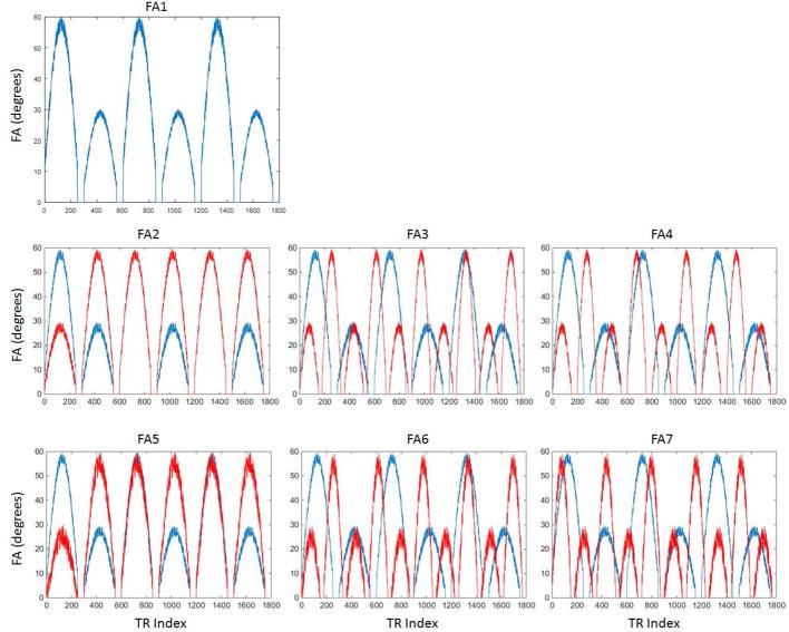
One unique feature of the MRF is the use of pseudo-randomized flip angle series. Theoretically, the resulting T1 and T2 values should be relatively independent of the choice of flip angles, as long as the pattern can generate sufficient differences between the signal evolutions from different tissues. However, the slice profile effect on the signal time-course may vary when different flip angle series are applied, especially when large flip angles are used. The slice profile effect from the flip angle train was investigated by changing the flip angle amplitude, duration of the sine-waveform, and the random perturbation from the original FA pattern used in ref(1). The same phantom set was scanned by MRF with seven flip angle (FA) series, with different angle values but with the same RF duration of 2000 us and TBW of 8. As shown in Figure 1, FA1 is the original FA pattern used in ref(1), with sine-waves duration of 250 TRs, intervals of 50 TRs where the flip angle was set to zeros, and a random perturbation with standard deviation (std) of 5 degrees. FA2 has a different flip angle amplitude as compared to FA1. FA3 and FA4 have narrower flip angle lobes (150 TRs) and shorter lengths for the zero flip angle (30 TRs), and FA5 to FA7 have increased flip angle oscillation (std of 10 degrees). The resulting T1 and T2 values with and without slice profile/B1 correction were compared. The coefficient of variation (CV) of T1 and T2 from each phantom was calculated as the standard deviation among the seven flip angle series divided by the standard value, and the agreement of T1 and T2 values of seven flip angles was evaluated as the average CV of all phantoms.
Figure 1.
Finally, to validate the repeatability of the MRF scans, MRF as well as standard T1 and T2 measurements were repeated in five consecutive days, each day with three repetitions. An RF pulse with duration of 2000 us and TBW of 8 was used for all of the repeatability tests. The mean and standard deviation of T1 and T2 values along the 15 repetitions were compared to those from the standard measurements. The concordance correlation coefficients (CCC) between the values from MRF and standard measurements were calculated.
In vivo studies
The in vivo experiments were performed in four asymptomatic volunteers in an IRB-approved study, including written informed consent before each scan. B1 measurement and MRF scans with RF pulses with duration of 2000 us and TBW of 8 were performed at the same slice location. The total acquisition time was 1.8 and 40 seconds for the B1 and MRF scans, respectively. In the T1 and T2 maps from each volunteer, four white matter regions (two in the frontal and two in the parietal white matter) and two gray matter regions were selected. The T1 and T2 values in each tissue type were first averaged for each volunteer, and then the mean and standard deviation of T1 and T2 values among four volunteers were calculated.
Post-processing
The post-processing was the same for both phantom and in vivo studies. All the acquired data were reconstructed using the non-uniform Fast Fourier Transform (NUFFT) with separately measured spiral trajectories(33). The reconstructed images were then projected to the SVD space to match the compressed dictionary(31,32). For the dictionary without slice profile and B1 simulation, the inner-product was calculated between the signal from each pixel and each element from the dictionary. For the dictionary which contains both B1 and the slice profile effects, the measured B1 map was used to choose a subdictionary for matching at each pixel. The maximum inner-product value from the match gave rise to T1, T2, off-resonance and M0 values. The computing time was 3.8 seconds and 7.8 minutes for the dictionary without and with slice profile/B1 simulation on a standalone PC, respectively.
Results
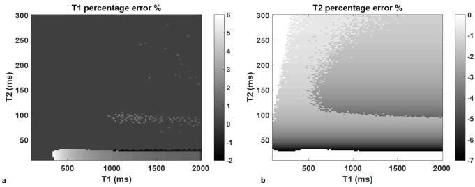
Figure 2 shows the T1 and T2 percent errors from a 2% change in B1 over the range of T1 from 100 to 2000 ms and T2 from 10 to 300 ms. T1 is relatively insensitive to such small B1 variations except for T2 values less than 30 ms, in which case the percent error of T1 is about 5.8%. The T2 error varies between −7.1% to 0%, with the least error noted at combinations of high T1, low T2 and low T1, or high T2.
Figure 2.
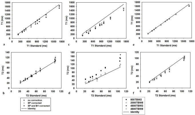
Figure 3(a) and (b) demonstrate the change of T1 and T2 values after the slice profile (SP) and B1 corrections from an RF pulse with a duration of 2000 us and TBW of 8. The B1 map of the phantom set is smooth with an average B1 close to 1 and a variation within the range between −2% to 3%. This only changes the T1 values by less than 1% and T2 by up to 5%. Therefore, the T1 and T2 values after SP correction and after both SP and B1 corrections are very similar. To demonstrate the results from four different RF pulses, T1 and T2 values obtained from the phantom scans before correction (Fig 3(c) and (d)) and after both SP and B1 corrections (Fig 3(e) and (f)) were compared to those from the standard measurements. The CCC and average percent difference of T1 and T2 values between MRF and standard measurements are listed in Table 1. Without any corrections, T1 is underestimated and T2 is overestimated with four of the RF pulses tested. all types of RF pulses. The results from the Sinc pulse with TBW of 2 deviate the most from the standard values. As shown in Table 1, the average percent difference compared to the standard is up to 27.9% for T1 and 47.6% for T2 from an RF pulse with TBW of 2. In general, after all corrections, T1 and T2 values from different pulses are more consistent and are in a good agreement with the standard values.
Figure 3.
Table 1.
The Concordance correlation coefficients (CCC) and average percent difference between the MRF results from four different RF profiles and standard measurements, before and after corrections.
| CCC | 800TBW2 | 2000TBW8 | 4800TBW2 | 4800TBW8 | |
|---|---|---|---|---|---|
| T1 | before | 0.911 | 0.954 | 0.875 | 0.950 |
| after | 0.996 | 0.997 | 0.997 | 0.998 | |
| T2 | before | 0.755 | 0.978 | 0.704 | 0.961 |
| after | 0.986 | 0.998 | 0.952 | 0.974 | |
| Average Percent Difference | 800TBW2 | 2000TBW8 | 4800TBW2 | 4800TBW8 | |
| T1 | before | −24.9% | −15.6% | −27.9% | −14.3% |
| after | −1.8% | −2.7% | −2.3% | −0.7% | |
| T2 | before | 43.1% | 7.8% | 47.6% | 9.5% |
| after | −8.8% | −2.2% | −14% | −9.1% | |
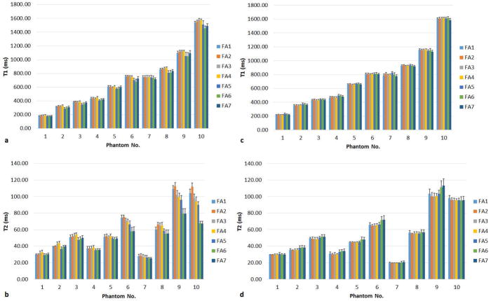
Figure 4 compares the T1 and T2 values from the phantom scans performed using the seven different flip angle series, without (a,b) and with (c,d) SP and B1 corrections. Before any corrections are applied, T1 and T2 values vary with FA patterns. Furthermore, comparing results between FA1 to FA4 and FA5 to FA7, a clear deviation can be seen from the flip angle patterns with an increased oscillation. The average CV of all phantoms was 2.86% for T1 and 7.52% for T2, respectively, before correction. After correction, the consistency of the T1 and T2 results across all flip angle series is improved, with an average CV of 1.29% for T1 and 2.94% for T2, respectively.
Figure 4.
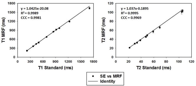
Figure 5 shows results from the repeatability study, with bi-directional error bars representing the standard deviation of all measurements (though they are on the order of the size of the marker in each case.) MRF results are in agreement with the results from the standard measurements, with a CCC of 0.99 for both T1 and T2. In addition, both MRF and standard measurements demonstrate high repeatability. The coefficient of variation (CV) is 1.17% for T1 and 3.08% for T2 from MRF scans.
Figure 5.
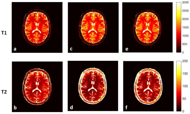
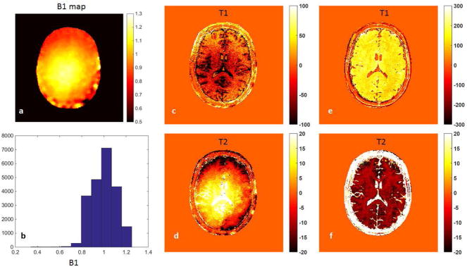
Figure 6 shows the results from one volunteer, showing the T1 and T2 maps without any correction (a,b), with only SP correction (c,d) and with both SP and B1 corrections (e,f). The B1 map and B1 distribution from the same subject is shown in Figure 7 (a) and (b), respectively. In order to demonstrate the slice profile and B1 effects separately, Figure 7(c,d) shows the change in results due to only the B1 correction, while Figure 7(e,f) shows the change in results due to only the SP correction. The SP correction uniformly increases T1 values and reduces T2 values, while the B1 correction in general reduces T1 and increases T2, with a similar local change as the B1 map shown in Figure 7(a). Table 2 compares the T1 and T2 values, with and without correction, from gray matter and white matter to those values from literature (2,34,35).
Figure 6.
Figure 7.
Table 2.
In vivo T1 and T2 values obtained from the MRF at 3T and the corresponding values reported in the literature
Discussion
In this work, we analyzed and corrected for the slice profile imperfection and local B1 inhomogeneity in the MRF sequence with a TrueFISP readout. While previous work(16) has solved this problem by using a train of B1 sensitive pulses and estimates all parameters at once, we used a two-step correction in our approach. Although a separate scan to measure B1 takes an additional 20 seconds, it reduces the sensitivity to potential tissue or system parameters, and thus reduces the amount of information and acquisition time required for the MRF scan. In addition, a prior knowledge of the B1 map reduces the dimensionality of the dictionary in pattern matching to estimate the tissue properties, which can lower the risk of mismatch and error propagation, especially in the present of strong aliasing artifacts and with low SNR from accelerated scans.
There are various methods available to measure B1 and actual flip angles. Besides the Bloch-Siegert method, other B1 mapping methods that are independent of the RF profile could also be used to provide a B1 map. Actual flip angle measurements(5,6,13) could theoretically account for both B1 and the slice profile. However, for MRF sequences with large flip angle variations, the scaling factor measured from a single flip angle may not accurate to apply to all other flip angles.
The phantom studies shown here mainly demonstrate the slice profile effect on T1 and T2 values, as the B1 variations are less than 3%. Since one often desires a fast acquisition in quantitative imaging and reduced banding artifacts from bSSFP-based sequences, the RF pulse used could be short with a poor slice profile. Here it was shown that this could induce an error in the quantitative result as high as 47.6%. Even from an RF pulse with a duration of 2000 us and TBW of 8, which is usually assumed to have a high-quality slice profile, the average percent difference compared to the standard is 13.6% and 8.0% for T1 and T2, respectively before correction. Precalculation of the slice profile into the dictionary improves the quantitative results significantly. The T1 and T2 results are in good agreement with the standard measurements independent of the type of the RF pulse used in the scan.
The phantom study also shows that, after corrections, the T1 and T2 results are largely independent of the choice of RF excitation pattern in the MRF scan, which provides more flexibility on how to design the excitation pattern. Although the B1 variation is not significant in the phantom study, the quantification of B0 in the TrueFISP-based sequence and the correction of B1 minimize the quantitative errors due to system variations, resulting in high reproducibility as shown in Figure 4.
The B1 inhomogeneity introduces a ±20% change in the flip angle variation in the in vivo study, which causes the actual flip angle to be as high as 72 degrees. As this study used the Bloch equations for simulation, with an incremental calculation of the RF-excitation, including relaxation and dephasing from gradients and off-resonance, there is no restriction on the range of flip angle. However, there is a tradeoff between a high flip angle and a good slice profile due to the limit of the transmit voltage.
Compared to the phantom results, B1 variation is not negligible in the in vivo study, so both slice profile and B1 corrections are essential to ensure the accuracy of the estimate. There are two main differences between the slice profile and B1 effects based on the in vivo results. First, the slice profile effect is uniform while the B1 effect is location-dependent and not necessarily symmetric; second, the slice profile and B1 have opposite effects on T1 and T2 values. Although we have shown an improved accuracy of T1 and T2 quantification after the slice profile and B1 corrections in the phantom study, we have noticed that in the in vivo study, the T1 and T2 results after corrections deviate more from the literature reported values. Since T1 and T2 quantification using traditional methods are difficult in vivo due to the time constraints, this large variation may be due to the variety of methods that have been used for in vivo T1 and T2 measurements, where some are more sensitive to slice profile and B1 effects than others. Other groups have seen lower T2 values after corrections for stimulated echoes(36), slice profile(21), magnetization transfer(37) and finite RF pulse effect(38). The low T2 values may also be related to micro structures and local field inhomogeneity. Recently, a pseudo-SSFP MRF sequence that simulated intra voxel dephasing has shown increased T1 and T2 results(39) as compared to those from the TrueFISP-based MRF with no slice profile and B1 corrections. An exact comparison of these results is the subject of a future investigation.
Finally, the main change in dictionary simulation includes the slice profile and contains the additional dimension of B1 values. Based on the B1 sensitivity study, a 2% step size of B1 was used in this study. Since the B1 sensitivity is dependent on the sequence design and acquisition parameters, such as flip angles and TRs, the step size of B1 and the size of the dictionary may change when a different sequence is used. Most of this increased computation burden happens before the data is actually acquired, and can be shared among all acquisitions of the same sequence. However, it is clear that computing clusters and GPUs can be used to accelerate both the dictionary simulation and the pattern matching steps, since both steps are highly parallelizable. In addition, the use of SVD compression(31) and fast group matching(32) can both dramatically accelerate the post-processing of MRF data.
Conclusion
This study demonstrated that MRF is sensitive to both slice profile and B1 effects. These effects cause deviations of actual flip angles from the nominal flip angles, have different sources of error and require different correction methods. By simulating the slice profile into the dictionary without adding scanner time, the sensitivity to the shape of the RF pulse and flip angle variations can be substantially reduced. In combination with a B1 mapping method, which further reduces the system and subject related variations, the suggested method improves both accuracy and robustness of the MRF results.
Acknowledgments
Support for this study was provided by NIH 1R01EB016728-01A1, NIH 5R01EB017219-02 and Siemens Healthcare. This work made use of the High Performance Computing Resource in the Core Facility for Advanced Research Computing at Case Western Reserve University.
References
- 1.Ma D, Gulani V, Seiberlich N, Liu K, Sunshine JL, Duerk JL, Griswold MA. Magnetic Resonance Fingerprinting. Nature. 2013;495:187–192. doi: 10.1038/nature11971. [DOI] [PMC free article] [PubMed] [Google Scholar]
- 2.Jiang Y, Ma D, Seiberlich N, Gulani V, Griswold Ma. MR fingerprinting using fast imaging with steady state precession (FISP) with spiral readout. Magn Reson Med. 2014 doi: 10.1002/mrm.25559. n/a-n/a. [DOI] [PMC free article] [PubMed] [Google Scholar]
- 3.Chen Y, Jiang Y, Pahva Shivani MaD, Lu L, Tweig MD, Wright KL, Seiberlich N, Griswold MA, Gulani V. MR Fingerprinting for Rapid Quantitative Abdominal Imaging. Radiology. 2016;0:1–9. doi: 10.1148/radiol.2016152037. [DOI] [PMC free article] [PubMed] [Google Scholar]
- 4.Wang J, Mao W, Qiu M, Smith MB, Constable RT. Factors Influencing Flip Angle Mapping in MRI: RF Pulse Shape, Slice-Select Gradients, Off-Resonance Excitation, and B0 Inhomogeneities. Magn Reson Med. 2006;56:463–8. doi: 10.1002/mrm.20947. [DOI] [PubMed] [Google Scholar]
- 5.Hornak JP, Szumowski J, Bryant RG. Magnetic Field Mapping. Magn Reson Med. 1988;6:158–163. doi: 10.1002/mrm.1910060204. [DOI] [PubMed] [Google Scholar]
- 6.Cunningham CH, Pauly JM, Nayak KS. Saturated double-angle method for rapid B1+ mapping. Magn Reson Med. 2006;55:1326–1333. doi: 10.1002/mrm.20896. [DOI] [PubMed] [Google Scholar]
- 7.Jiru F, Klose U. Fast 3D Radiofrequency Field Mapping Using Echo-Planar Imaging. Magn Reson Med. 2006;56:1375–1379. doi: 10.1002/mrm.21083. [DOI] [PubMed] [Google Scholar]
- 8.Dowell NG, Tofts PS. Fast, Accurate, and Precise Mapping of the RF Field in vivo using the 180 Degrees Signal Null. Magn Reson Med. 2007;58:622–630. doi: 10.1002/mrm.21368. [DOI] [PubMed] [Google Scholar]
- 9.Morrell GR. A Phase-Sensitive Method of Flip Angle Mapping. Magn Reson Med. 2008;60:889–894. doi: 10.1002/mrm.21729. [DOI] [PubMed] [Google Scholar]
- 10.Park J-Y, Garwood M. B1 Mapping Using Phase Information Created by Frequency-Modulated Pulses. Proceedings 16th Scientific Meeting, International Society for Magnetic Resonance in Medicine. 2008;16:361. [Google Scholar]
- 11.Sacolick LI, Wiesinger F, Hancu I, Vogel MW. B1 mapping by Bloch-Siegert Shift. Magn Reson Med. 2010;63:1315–1322. doi: 10.1002/mrm.22357. [DOI] [PMC free article] [PubMed] [Google Scholar]
- 12.Ganter C, Settles M, Dregely I, Santini F, Scheffler K, Bieri O. B1+-Mapping with the Transient Phase of Unbalanced Steady-State Free Precession. Magn Reson Med. 2013;0:1–9. doi: 10.1002/mrm.24598. [DOI] [PubMed] [Google Scholar]
- 13.Yarnykh VL. Actual Flip-Angle Imaging in the Pulsed Steady State: a Method for Rapid Three-Dimensional Mapping of the Transmitted Radiofrequency Field. Magn Reson Med. 2007;57:192–200. doi: 10.1002/mrm.21120. [DOI] [PubMed] [Google Scholar]
- 14.Nehrke K. On the Steady-State Properties of Actual Flip Angle Imaging (AFI) Magn Reson Med. 2009;61:84–92. doi: 10.1002/mrm.21592. [DOI] [PubMed] [Google Scholar]
- 15.Hurley Sa, Yarnykh VL, Johnson KM, Field AS, Alexander AL, Samsonov Aa. Simultaneous Variable Flip Angle-Actual Flip Angle Imaging Method for Improved Accuracy and Precision of Three-Dimensional T1 and B1 Measurements. Magn Reson Med. 2012;68:54–64. doi: 10.1002/mrm.23199. [DOI] [PMC free article] [PubMed] [Google Scholar]
- 16.Buonincontri G, Sawiak SJ. MR fingerprinting with simultaneous B1 estimation. Magn Reson Med. 2015;0:1–9. doi: 10.1002/mrm.26009. [DOI] [PMC free article] [PubMed] [Google Scholar]
- 17.Cloos MA, Knoll F, Zhao T, Block K, Bruno M, Wiggins C, Sodickson D. Multiparametric imaging with heterogeneous radiofrequency field: Additional material. Nat Commun. 2016 doi: 10.1017/CBO9781107415324.004. [DOI] [PMC free article] [PubMed] [Google Scholar]
- 18.Bieri O, Scheffler K. SSFP Signal With Finite RF Pulses. Magn Reson Med. 2009;62:1232–41. doi: 10.1002/mrm.22116. [DOI] [PubMed] [Google Scholar]
- 19.Staehle F, Leupold J, Hennig J, Markl M. Off-resonance-dependent slice profile effects in balanced steady-state free precession imaging. Magn Reson Med. 2008;59:1197–1202. doi: 10.1002/mrm.21557. [DOI] [PubMed] [Google Scholar]
- 20.Mcrobbie DW, Lerski RA, Robinson EM, Hickey DS, Lerski RA, Bakker CJG, De Graaf CN, Van Dijk P. Slice Profile Effects and Their Calibration and Correction in Quantitative NMR NMR Imaging. Phys Med Biol. 1987;32:971–983. [Google Scholar]
- 21.Ehses P, Seiberlich N, Ma D, Breuer FA, Jakob PM, Griswold MA, Gulani V. IR TrueFISP with a golden-ratio-based radial readout: fast quantification of T1, T2, and proton density. Magn Reson Med. 2013;69:71–81. doi: 10.1002/mrm.24225. [DOI] [PubMed] [Google Scholar]
- 22.Tannús A, Garwood M. Adiabatic Pulses. NMR Biomed. 1997;10:423–34. doi: 10.1002/(SICI)1099-1492(199712)10:8<423::AID-NBM488>3.0.CO;2-X. [DOI] [PubMed] [Google Scholar]
- 23.Norris DG. Adiabatic radiofrequency pulse forms in biomedical nuclear magnetic resonance. Concepts Magn Reson. 2002;14:89–101. doi: 10.1002/cmr.10007. [DOI] [Google Scholar]
- 24.Hong T, Kim M-O, Han D, Hwang D, Kim D-H. B1+ inhomogeneity compensated MRF using simultaneous AFI. Proceedings 23rd Scientific Meeting, International Society for Magnetic Resonance in Medicine Scientific Meeting, International Society for Magnetic Resonance in Medicine; 2015. p. 3248. [Google Scholar]
- 25.Hong T, Kim M-O, Han D, Kim D-H. Analysis of estimation error from system imperfection in MRF. Proceedings 24th Scientific Meeting, International Society for Magnetic Resonance in Medicine; 2016. p. 437. [Google Scholar]
- 26.Pauly JM, Le Roux P, Nishimura DG, Macovski A. Parameter Relations for the Shinnar-Le Roux Selective Excitation Pulse Design Algorithm. IEEE Trans Med Imaging. 1991;10:53–65. doi: 10.1109/42.75611. [DOI] [PubMed] [Google Scholar]
- 27.Shinnar M, Bolinger L, Leigh JS. The Use of Finite Impulse Response Filters in Pulse Design. Magn Reson Med. 1989;12:81–87. doi: 10.1002/mrm.1910120110. [DOI] [PubMed] [Google Scholar]
- 28.Christen T, Pannetier Na, Ni WW, Qiu D, Moseley ME, Schuff N, Zaharchuk G. MR Vascular Fingerprinting: A New Approach to Compute Cerebral Blood Volume, Mean Vessel Radius, and Oxygenation Maps in the Human Brain. Neuroimage. 2014;89:262–70. doi: 10.1016/j.neuroimage.2013.11.052. [DOI] [PMC free article] [PubMed] [Google Scholar]
- 29.Gao Y, Chen Y, Ma D, et al. Preclinical MR fingerprinting (MRF) at 7 T: effective quantitative imaging for rodent disease models. NMR Biomed. 2015;28:384–94. doi: 10.1002/nbm.3262. [DOI] [PMC free article] [PubMed] [Google Scholar]
- 30.Lee JH, Hargreaves BA, Hu BS, Nishimura DG. Fast 3D imaging using variable-density spiral trajectories with applications to limb perfusion. Magn Reson Med. 2003;50:1276–85. doi: 10.1002/mrm.10644. [DOI] [PubMed] [Google Scholar]
- 31.McGivney D, Pierre E, Ma D, Jiang Y, Saybasili H, Gulani V, Griswold MA. SVD Compression for Magnetic Resonance Fingerprinting in the Time Domain. IEEE Trans Med Imaging. 2014;62:1–13. doi: 10.1109/TMI.2014.2337321. [DOI] [PMC free article] [PubMed] [Google Scholar]
- 32.Cauley SF, Setsompop K, Ma D, Jiang Y, Ye H, Adalsteinsson E, Griswold Ma, Wald LL. Fast Group Matching for MR Fingerprinting Reconstruction. Magn Reson Med. 2014;0:1–6. doi: 10.1002/mrm.25439. [DOI] [PMC free article] [PubMed] [Google Scholar]
- 33.Duyn JH, Yang Y, Frank JA, van der Veen JW. Simple Correction Method for k-Space Trajectory Deviations in MRI. J Magn Reson. 1998;132:150–3. doi: 10.1006/jmre.1998.1396. [DOI] [PubMed] [Google Scholar]
- 34.Wansapura JP, Holland SK, Dunn RS, Ball WS. NMR Relaxation Times in the Human Brain at 3.0 Tesla. J Magn Reson Imaging. 1999;9:531–8. doi: 10.1002/(sici)1522-2586(199904)9:4<531::aid-jmri4>3.0.co;2-l. [DOI] [PubMed] [Google Scholar]
- 35.Hasan KM, Walimuni IS, Kramer La, Narayana Pa. Human brain iron mapping using atlas-based T2 relaxometry. Magn Reson Med. 2012;67:731–9. doi: 10.1002/mrm.23054. [DOI] [PMC free article] [PubMed] [Google Scholar]
- 36.Ben-Eliezer N, Sodickson DK, Block KT. Rapid and accurate T2 mapping from multi-spin-echo data using bloch-simulation-based reconstruction. Magn Reson Med. 2015;73:809–817. doi: 10.1002/mrm.25156. [DOI] [PMC free article] [PubMed] [Google Scholar]
- 37.Gloor M, Scheffler K, Bieri O. Quantitative Magnetization Transfer Imaging Using Balanced SSFP. Magn Reson Med. 2008;60:691–700. doi: 10.1002/mrm.21705. [DOI] [PubMed] [Google Scholar]
- 38.Crooijmans HJa, Scheffler K, Bieri O. Finite RF pulse correction on DESPOT2. Magn Reson Med. 2011;65:858–62. doi: 10.1002/mrm.22661. [DOI] [PubMed] [Google Scholar]
- 39.Assländer J, Glaser SJ, Hennig J. Pseudo Steady-State Free Precession for MR-Fingerprinting. Magn Reson Med. 2016;0:1–11. doi: 10.1002/mrm.26202. [DOI] [PubMed] [Google Scholar]


