Robust total retina thickness segmentation in optical coherence tomography images using convolutional neural networks

Abstract

We developed a fully automated system using a convolutional neural network (CNN) for total retina segmentation in optical coherence tomography (OCT) that is robust to the presence of severe retinal pathology. A generalized U-net network architecture was introduced to include the large context needed to account for large retinal changes. The proposed algorithm outperformed qualitative and quantitatively two available algorithms. The algorithm accurately estimated macular thickness with an error of 14.0 ± 22.1 µm, substantially lower than the error obtained using the other algorithms (42.9 ± 116.0 µm and 27.1 ± 69.3 µm, respectively). These results highlighted the proposed algorithm’s capability of modeling the wide variability in retinal appearance and obtained a robust and reliable retina segmentation even in severe pathological cases.

1. Introduction

Optical coherence tomography (OCT) has become a key diagnostic imaging technique for the diagnosis of retinal diseases [1]. Its ability to visualize the internal structure of the retina allows for a qualitative and quantitative assessment of morphological changes associated with underlying diseases [2]. OCT-derived measures are widely accepted in clinical practice and clinical trials as pivotal markers for the assessment of treatment response and disease progression [3, 4]. Particularly, retinal thickness or central macular thickness (CMT) as measured in OCT has been demonstrated to correlate with pathological changes and treatment outcome for a variety of ocular diseases [5–7].

For quantitative thickness measurements in OCT, retina segmentation is required to accurately delimit the retinal extension, distinguishing it from other eye structures, such as choroidal or vitreous tissue. Automated methods for thickness quantification currently available in clinical and research environments rely on the accurate identification of the inner and outer retinal boundaries using layer segmentation algorithms. Retinal thickness is then estimated as the space between the detected surfaces.

However, recent work has demonstrated that current commercially available retinal layer segmentation algorithms have a large number of segmentation errors, especially in the presence of neurodegenerative diseases such as AMD [8, 9], rendering the derived thickness measurements unreliable [10, 11]. The presence of large disruptive pathology such as subretinal fluid, intraretinal cysts and retinal detachments disrupts the logical structured organization of the retinal layers causing many segmentation algorithms to fail. Precise manual corrections of the erroneous segmentation is then required to prevent misleading outcomes [7], which is time consuming, undesirable and even unfeasible in large scale population studies. There is therefore a need to develop robust segmentation techniques for retinal thickness estimation especially in the presence of severe disruptive pathology [8].

Existing research retinal layer segmentation algorithms can be roughly subdivided into two categories, mathematical modeling approaches and machine learning approaches [12]. Mathematical modeling attempts to capture the typical layered structure of the retina in a model based on the anatomical, structural and clinical prior knowledge that is known about the retina. Capturing all the possible variations in retinal appearance in a single mathematical model can be challenging, especially for severe changes and abnormalities that can be present in disruptive retinal diseases such as age related macular degeneration (AMD).

Mathematical modeling based approaches for healthy or retinas with mild pathology include A-scan methods [13, 14], Markov modeling [15], algorithms based on active contour modeling [16], methods using sparse high order potentials [17], variational methods [18] and approaches using graph theory [12, 19–22]. Especially the last ones have shown excellent results in segmenting the individual retinal layers [23]. Typically, graph theoretic approaches implement certain predetermined constraints to obtain smooth surfaces or constrain the layers to have a certain distance to each other [19, 24–26]. While these constraints typically improve segmentation accuracy, they do place a limit on the allowable deformation of the retina and tend to fail in the presence of large abnormalities [27]. For that reason, methods based on mathematical modeling have been modified to integrate model variants robust to these abnormalities, for example by integrating sparse higher order potentials to cope with local boundary variations [27], or by adapting the graph theory and dynamic programming framework to specifically model drusen and fluid in the retina [28–31]. Combinations of mathematical modeling and machine learning have also been explored to improve the performance in the presence of abnormalities. Typically, the output of a machine learning approach was required as initialization for a consecutive graph search to accurately identify retinal layers [32–35].

Pure machine learning algorithms for retinal layer segmentation typically do not estimate the retinal boundaries by fitting a line directly, but classify each pixel in an image as belonging to a certain layer or boundary by training a supervised classifier on features extracted from that pixel. Traditional classifiers, such as a support vector machine, random forest or neural network, have also been proposed for the segmentation of the retinal layers [36–39], but scarcely in the presence of retinal abnormalities [40].

In recent years, deep learning methods, especially convolutional neural networks (CNNs), have gained popularity in the field of computer vision [41] and are now also entering the field of retinal image analysis [42–44]. In deep learning hierarchical features are learned directly from the training data, building a complex classifier that is capable of capturing the large variability in the training data, e.g., disruptive pathology in OCT images. Few CNN algorithms have been specifically proposed for retinal segmentation but always in combination wit graph theory. A single-scale patch based CNN in combination with graph search [45] has been proposed for the segmentation of intraretinal layers in non-exudate AMD with good results. Instead of using gradient based edge weight for initializing the graph search, the probability map produced by the CNN is used to find the layer boundaries. However, the single-scale nature of this implementation limits the spatial context included to make a classification decision. A multi-scale CNN approach combined with graph search for the related problem of choroidal tissue segmentation [46] showed the importance of analyzing OCT images at multiple scales. The OCT image is provided to the network at several scales allowing analysis of the image with increasing contextual information. However, both approaches used the CNN output as an initialization for a graph theory approach.

In this work, we propose an a machine learning algorithm for total retina thickness segmentation using a CNN that is robust to severe disruptive retinal pathology. In contrast to mathematical modeling based approaches the proposed algorithm delimits the retina by performing a semantic segmentation of the OCT volume. Every pixel in each B-scan is directly classified as belonging to the retina or not, avoiding assumptions about the retinal structure and its layered organization. This absence of constraints and a priori knowledge allows for a flexible model that is capable of capturing the wide range of possible variations in retinal appearance when disruptive pathology is present.

The proposed CNN architecture builds upon U-net [47], a fully convolutional network for spatially dense prediction tasks. This architecture implements a multi-scale analysis of an image, allowing spatially distant information to be included in the classification decision but maintaining pixel accurate localization avoiding the need of an additional step based on graph search. We modify and extend this architecture to include a tailored spatial context which accounts for large retinal pathological changes while keeping computational requirements at a minimum. A consecutive graph search is not required to refine the segmentation boundaries. Specifically, we infer a closed form equation to determine the number of convolution and pooling layers in the proposed generalized U-net architecture needed to obtain a receptive field tailored to a given application.

The algorithm performance is evaluated in 1) a large private database of OCT scans from AMD patients with different disease severity levels including severe advanced AMD, and 2) a publicly available database containing OCT scans obtained from patients with DME. Segmentation accuracy is compared to two available algorithms, one commercially available and one extensively used in research settings.

2. Materials

2.1. Study dataset

OCT volume scans of patients with AMD and controls were randomly selected from the European Genetic Database (EUGENDA, http://eugenda.org), a large multi-center database for clinical and molecular analysis of AMD. The EUGENDA study was performed according to the tenets set forth in the Declaration of Helsinki, and approved by the Institutional Review Board. Written informed consent was obtained before enrolling patients in EUGENDA. OCT imaging was performed using Spectralis HRA+OCT (Heidelberg Engineering, Heidelberg, Germany) at a wavelength of 870 nm, transversal resolution ranging from 6 µm to 14 µm and an axial resolution of up to 3.9 µm. The number of B-scans (or slices) per volume varied from 19 to 38, corresponding to a B-scan spacing ranging from ~320 micron up to ~160 micron, respectively. The AMD severity level was graded for each OCT scan based on the assessment of a color fundus image acquired at the same time, following the Cologne Image Reading Center and Laboratory (CIRCL) grading protocol [48].

145 OCT volumes from 71 patients with advanced AMD were randomly selected for the development of the proposed algorithm. This set was further split into a training set of 130 OCT volumes and a validation set of 15 volumes for CNN training and monitoring, respectively. OCT volumes from the same patient were kept in the same subset. An independent test set of 99 OCT volumes from 99 patients was randomly selected for the evaluation of the algorithm performance. The OCT volumes were evenly extracted from different AMD severity levels, i.e., 33 scans were graded as early AMD or no AMD, 33 as intermediate AMD and 33 as advanced AMD. Before processing, all B-scans from an OCT volume were resampled to a constant pixel size of 11.5 µm × 3.9 µm.

To allow for comparison to other available methods an external set was used from a publicly available database [32] comprised of 10 OCT volumes obtained from patients with diabetic macular edema (DME) containing large visible intraretinal cysts. OCT volumes were acquired using a Spectralis HRA+OCT (Heidelberg Engineering, Heidelberg, Germany). For further details and information concerning the inclusion criteria we refer to the paper describing the data set [32].

2.2. Reference standard and observer annotations

For this study the retina was defined as the region between the inner limiting membrane (ILM) and the outer boundary of the retinal pigment epithelium (RPE) [49] (Fig. 1). Based on this definition, the retina was manually segmented in the training and validation set by a single experienced observer. In order to minimize annotation time, a semi-automated annotation approach was carried out, in which an initial segmentation was obtained using a research-based, publicly available algorithm [19] and provided to the grader in a custom workstation for manual corrections. The workstation allowed to visualize the B-scans with the initial segmentation and manually adjust it at any location throughout the scan.

Fig. 1.

The retina is defined as the region between the inner limiting membrane (ILM) and the outer boundary of the retinal pigment epithelium (RPE), including subretinal fluid but excluding retinal detachments. ILM and RPE are delineating in red on the OCT B-scan.

A second experienced observer manually segmented the retina in all the OCT volumes of the test set. As initial segmentations were not provided to this observer, only A-scans intersecting with the 1 mm circle surrounding the fovea were annotated in order to reduce the annotation workload.

3. Method

The proposed algorithm obtains full retina segmentation using a CNN architecture by performing a semantic segmentation, i.e., classifying each location in an OCT scan. The network receives a B-scan from an OCT volume as input and outputs a probability map indicating for each pixel in the scan the likelihood to be inside the retina. The final segmentation is obtained by smoothing and thresholding this probability map.

3.1. U-net architecture

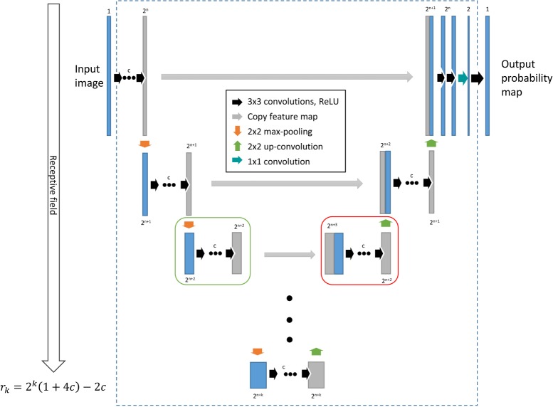
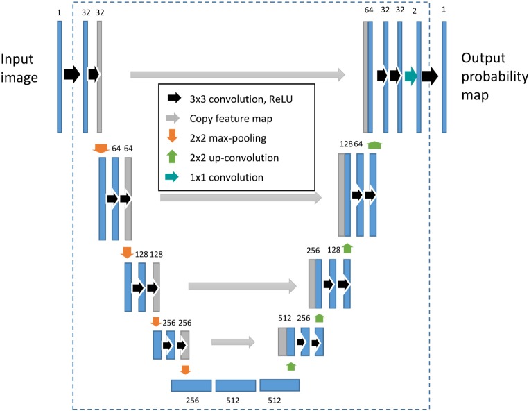
The proposed CNN architecture builds upon U-net [47], a fully convolutional network where local and contextual information is fused to obtain an accurate dense image segmentation. The typical U-net architecture consists of three components: 1) a contracting path to capture contextual information by successively reducing the size of the feature maps; 2) a symmetric expanding path for upsampling the low resolution feature map resulting from the contracting part to the full resolution of the input image; and 3) a connection path to combine feature maps from the contracting and expanding paths to incorporate local information and obtain accurate localization. Specifically, the contracting path consists of the repeated application of a 2×2 max pooling (MP) operation with stride 2 for downsampling [50] and two 3×3 convolutions (C3), each followed by a rectified linear unit (ReLU), i.e.,

$$MP\Rightarrow C3\Rightarrow ReLu\Rightarrow C3\Rightarrow ReLu$$ (1)

At each downsampling step the number of feature channels is doubled. The expanding path consists of an upsampling operation (U) of the feature map followed by a 2×2 convolution that halves the number of feature channels, a concatenation (CAT) with the corresponding feature map from the contracting path, and two 3×3 convolutions, each followed by a ReLU, i.e.,

$$U\Rightarrow C2\Rightarrow ReLu\Rightarrow CAT\Rightarrow C3\Rightarrow ReLu\Rightarrow C3\Rightarrow ReLu$$ (2)

At the final layer a 1×1 convolution is used to map each final feature vector to the desired number of classes. In total the network has 27 convolutional layers. Being fully convolutional, learning and inference are performed using whole images by dense feedforward computation and backpropagation, increasing processing speed compared to patch-based networks.

3.2. Generalized U-net architecture

As explained in the previous section, the contracting part is mainly responsible for incorporating wide spatial context by successively applying max pooling operations and thereby increasing its receptive field. For the original U-net architecture explained in [47] an effective receptive field of 140×140 pixels is obtained. For our data, this would correspond to a spatial context of 1.6 mm × 0.5 mm, which might not be enough to fully capture large disruptive abnormalities, such as fluid-filled spaces, that can expand from a few tens of microns to larger than 5 mm. In order to capture wider contextual information, we generalize the U-net architecture to obtain a receptive field tailored to the input data. Figure 2 shows a scheme of the proposed generalized U-net.

Fig. 2.

Generalized U-net architecture. The green and red boxes indicate the basic downsample and upsample units, respectively. The parameter c indicates the number of 3×3 convolutions in every unit. Making the network deeper by adding k more downsample units will increase the receptive field r_k according to Eq. (5).

Let a downsample unit in the generalized U-net architecture be the group of c 3×3 convolutions followed by a ReLU and a spatial max pooling layer with a 2×2 kernel size. Let k be the total number of downsample units. Considering that a single 3×3 convolution operation increases the receptive field by one pixel in all directions and a pooling operation halves the feature map and doubles the receptive field, the effective receptive field r_k after adding k downsample units is recursively defined as followed:

$$r_k=2(r_{k-1}+2c)$$ (3)

and can be written as a partial sum:

$$\begin{array}{l}{r}_k=2^k{r}_0+4c{\displaystyle \sum _{j=0}^{k-1}2j}\\ =2^k{r}_0+4c(2^k-1)\end{array}$$ (4)

where r₀ is the initial receptive field, i.e., 1 pixel. Adding the c convolutions at the input level, the receptive field r_k of the proposed generalized architecture can be expressed as a function of the number k of downsample units and the number c of convolutions per unit as follows:

$$r_k=2^k(1+4c)-2c$$ (5)

The original U-net architecture can be obtained in our generalized framework by setting c = 2 and k = 4, resulting in the architecture shown in Fig. 3. Equation (5) indicates the receptive field for this architecture is 140×140 pixels (1.6 mm × 0.5 mm). Taking into account that large abnormalities can cover a horizontal width of up to 5 mm, an receptive field of at least 5 mm is needed to introduce enough contextual information to account for these abnormalities. Given the pixel size of our data, that would mean a required receptive field of at least 435 pixels. Setting the number of convolution c = 2, the number of downsample units needed for our data would be k = 6. This will result in a receptive field of 572×572 pixels, large enough to capture enough contextual information even when large abnormalities are present.

Fig. 3.

Original U-net architecture. The original U-net architecture is obtained by setting c = 2 and k = 4 in the generalized U-net architecture, i.e., 2 convolutional layers per downsample unit, and 4 downsample units in total.

3.3. Network training process

The CNN was trained using RMSProp with a learning rate starting at 10⁻³ up to 10⁻⁶. The learning rate was manually decreased by a factor of 10 whenever a plateau was reached in the learning curve. Given a mini-batch $ℬ=B_1,\dots ,B_i,\dots ,B_m$ of m training B-scans B_i (x), a weighted loss function [47] was used for the network optimization:

$$C={\displaystyle \sum _{\forall x\in B_i,\forall B_i\in ℬ}{w}_i(\mathbf{x})\log \left(\left|{\tilde{S}}_i(\mathbf{x})-S_i(\mathbf{x})\right|\right)}$$ (6)

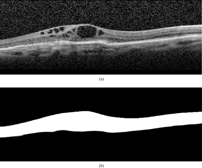
where S_i (x) is a binary image representing the annotated retina segmentation of B_i (x) and w_i (x) is the corresponding weight map for that scan. Figure 4 shows an example of a B-scan and its corresponding binary image S_i (x). The weight w_i (x) for pixel x in a training B-scan B_i (x) was defined as:

$$w_i(\mathbf{x})=\{\begin{array}{ll}\frac{N_{back}}{N_{ret}+N_{back}},& \text{if}{S}_i(\mathbf{x})=1,\text{i.e.},\mathbf{x}\in retina.\\ \frac{N_{ret}}{N_{ret}+N_{back}},& \text{if}{S}_i(\mathbf{x})=0,\text{i.e.},\mathbf{x}\in background.\end{array}$$ (7)

where N_ret and N_back are the number of pixels with S_i (x) = 1 and S_i (x) = 0, respectively. This weight map was used to balance the contribution of each class, i.e., retina or background, to the cost function and improved the convergence rate of the network parameters. To maximize the throughput of the GPU the mini-batch size was set to process six B-scans (m = 6) at the same time. Momentum was set to 0.99 in order to include a large amount of previously seen samples in the current update step. We used Glorot-normal initialization [51] for the weights of the network. Data augmentation by horizontal flipping was applied randomly to every B-scan during training to artificially increase the amount of training data. Prior to processing, the input B-scan was padded with zeros to ensure that every max pooling operation in the network was applied to a feature map with even horizontal and vertical dimensions. Even feature maps were required to have a one-to-one pixel correspondence when concatenating the feature maps in the expanding path of the network after upsampling. The padded zeros got a weight w of zero as they are not adding any information to the network. During training the validation set was used to monitor the training progress and to prevent overfitting. After every epoch the cost and the dice similarity overlap coefficient were calculated to determine convergence of the network. The network architecture and training procedures were implemented in Python 2.7 using the Theano [52] and Lasagne [53] packages for the deep learning framework. Training of the network was performed on a a Nvidia titan X GPU using CUDA 7.5 with cuDNN v4 and CNMeM optimizations enabled. Convergence of the network was reached in about 36 hours. Processing a single OCT volume comprised of 38 B-scans during training takes about 10 seconds, while a complete volume segmentation is produced in only 5 seconds during test time.

Fig. 4.

Example of a training B-scan B_i (a) and its corresponding binary image S_i (b) obtained from the provided manual annotations.

4. Post-processing

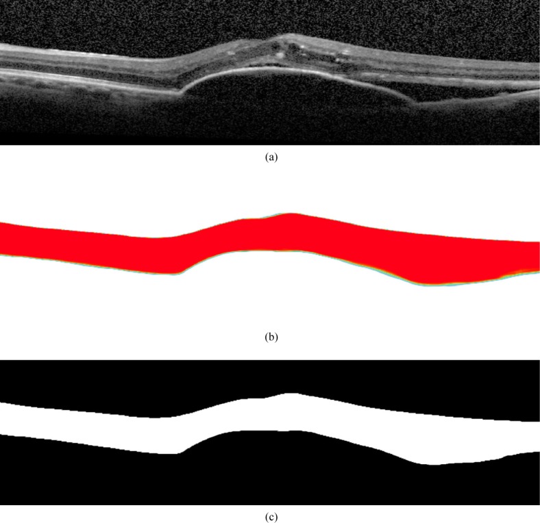
After applying the proposed generalized U-net architecture to an OCT volume the produced retina probability map is thresholded. An example of an input image, the produced probability map and the thresholded final output are shown in Fig. 5. To find the optimal threshold, the threshold value was varied between 0.5 and 1 in steps of 0.01. At each value the distance between the boundaries of the annotated segmentation and the estimated segmentation in the validation set was calculated. The value at which the distance between both boundaries was minimal was chosen as the optimal threshold. In our case the optimal threshold was found to be 0.98. This same threshold was used in processing the unseen test set. This value deviates from the typical 0.5 to offset the distribution bias [54] towards classifying pixels as belonging to the retina introduced by the class balancing described in Section 3.3 and Eq. (7).

Fig. 5.

Example of (a) an input image, (b) the corresponding probability map produced by the proposed algorithm, and (c) the final thresholded output.

5. Experimental design

The performance of the proposed algorithm for retina segmentation was qualitative and quantitatively assessed in the test set and compared to the performance of two widely used existing algorithms: the retina segmentation algorithm embedded in the clinically used Heidelberg Eye Explorer software version 1.9.10.0 (Heidelberg Engineering, Heidelberg, Germany) with HRA/Spectralis Viewing Module version 6.3.4.0 installed (Algorithm A), and the Iowa reference algorithm version 4.0 [23, 55, 56], which is often used in research settings (Algorithm B). No details about specifications and limitations of its use for both reference algorithms were found in the provided documentation.

The different algorithms were used to process the 99 OCT images in the test set and extract the retina segmentation, resulting in a total of 297 segmentation outputs.

Additionally, to allow for comparison to existing algorithms, the proposed algorithm was applied to the external set.

5.1. Qualitative assessment of the segmentation performance

As a qualitative evaluation of the algorithm performance, an experienced ophthalmologist visually rated the segmentation accuracy in the entire OCT scan by assigning an accuracy score to each segmentation output. The ophthalmologist was instructed to look for visually apparent deviations from the RPE and ILM segmentation boundaries. We did not set a strict threshold for the minimum boundary deviation still considered an error, but instead relied on the experience of the ophthalmologist to detect regions of segmentation failure with high sensitivity. This score was defined as 1) good if segmentation errors were made in 0 to 5% of the retina extension; 2) moderate if the errors were present in 5 to 15% of the retina extension; and 3) failure if the errors were present in more than 15% of the retina extension. To assign the accuracy score, the segmentation outputs of each algorithm were imported to an in-house developed workstation and presented in a random order to the observer for blind assessment.

5.2. Quantitative assessment of segmentation performance

To quantitatively assess the robustness of the segmentation algorithm, central macular thickness (CMT) measurements derived from the obtained retina segmentation were calculated and compared to the manual annotations made by an experienced grader. The location of the fovea, which is required to determine the CMT, was selected manually.

Global performance was assessed by calculating the mean absolute difference in CMT thickness compared to the manual reference, the intraclass correlation coefficient (ICC) between the manual CMT and the CMT derived from the different algorithms, and Bland-Altman statistics in the entire test set for the different AMD severity levels. Additionally we looked at the total segmented area and calculated the Dice overlap coefficient [57] between the manually annotated retina area and the segmentation output for the different algorithms. Finally, to analyze the agreement with the reference annotation in detecting the specific boundaries, i.e., the ILM and RPE, the mean absolute distance to the manual reference annotation was calculated on A-scan level for both boundaries separately.

The Dice overlap coefficient and the mean absolute distances were also calculated in the external set and compared to the human reference and automatic segmentation results provided with the publicly available dataset.

6. Results

6.1. Qualitative assessment of the segmentation performance

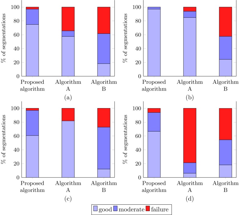
Figure 6(a) summarizes the qualitative assessment of the segmentation outputs obtained with the proposed algorithm and Algorithm A and B. The accuracy of the proposed algorithm was considered good to moderate in 97.0% of the OCT scans in the test set, compared to the 65.6% and 61.6% obtained with Algorithms A and B, respectively. Figures 6(b)–6(d) show the segmentation accuracy in OCT scans with different AMD severity levels. Manual annotations by a human grader for the central 1 mm region surrounding the fovea are indicated in green.

Fig. 6.

Qualitative assessment of segmentation performance (a) for all OCT volumes in the test set, (b) for OCT volumes with no pathology or signs of early AMD, (c) for OCT volumes with intermediate AMD, (d) for OCT volumes with advanced AMD.

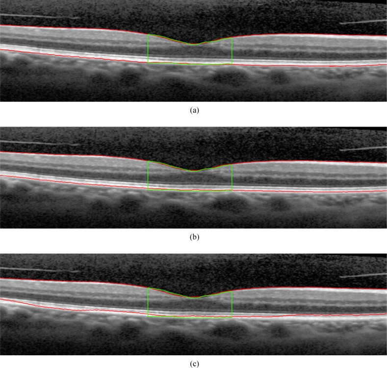
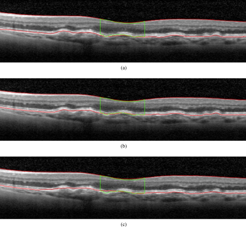
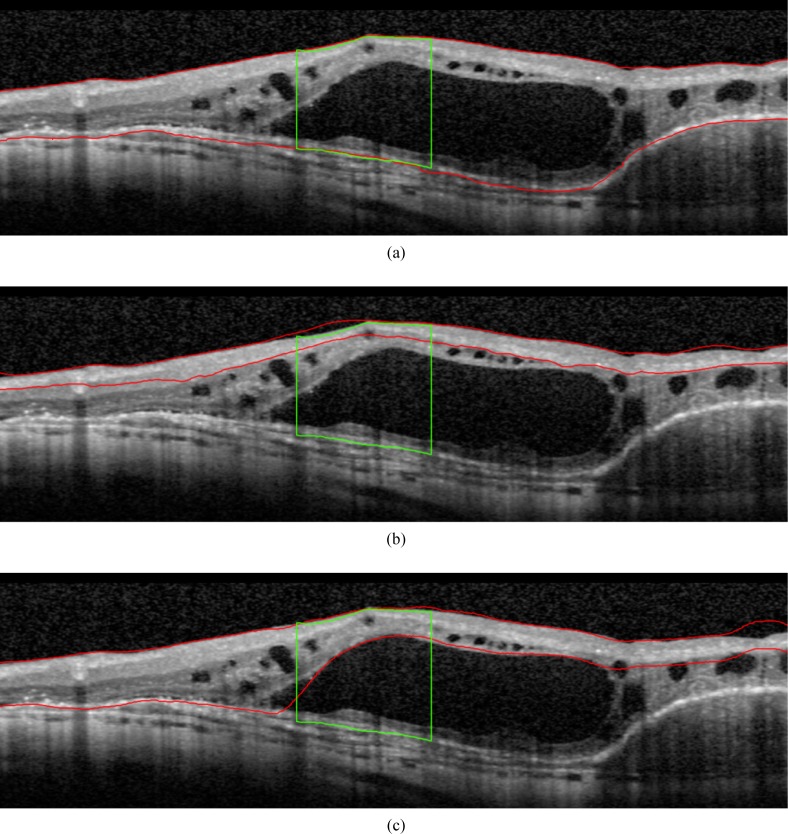
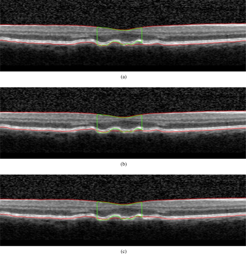
In the presence of advanced AMD, the segmentation output for Algorithm A was rated as a failure in 78.7% of the cases and in 45.5% for Algorithm B, whereas the output of the proposed algorithm was only rated as failure in 6.1% of the advanced case. Figures 7, 8 and 9 show examples of the retina segmentation obtained with each algorithm for cases with early, intermediate and advanced AMD, respectively.

Fig. 7.

Examples of B-scans showing the segmentation performance of the three different algorithms for the subgroup of early AMD: (a) Proposed algorithm, (b) Algorithm A, (c) Algorithm B. The segmentation boundaries are shown in red, while the manual annotation of A-scans intersecting with the 1 mm circle surrounding the fovea are shown in green.

Fig. 8.

Examples of B-scans showing the segmentation performance of the three different algorithms for the subgroup of intermediate AMD: (a) Proposed algorithm, (b) Algorithm A, (c) Algorithm B. The segmentation boundaries are shown in red, while the manual annotation of A-scans intersecting with the 1 mm circle surrounding the fovea are shown in green.

Fig. 9.

Examples of B-scans showing the segmentation performance of the three different algorithms for the subgroup of advanced AMD: (a) Proposed algorithm, (b) Algorithm A, (c) Algorithm B. The segmentation boundaries are shown in red, while the manual annotation of A-scans intersecting with the 1 mm circle surrounding the fovea are shown in green.

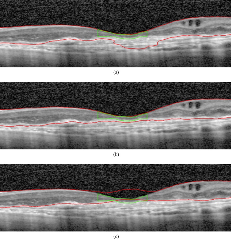
Figure 10 shows the single case graded by the human observer as failure for the proposed method in the subgroup of intermediate AMD. The segmentation results obtained by Algorithm A and Algorithm B are also included. Figure 11 shows one of the two cases graded by the human observer as failure for the proposed method in the subgroup of advanced AMD. The segmentation results obtained by the two reference algorithms are also included.

Fig. 10.

Example of a failed case for (a) the proposed method in the subgroup of intermediate AMD together with the segmentation produced by (b) Algorithm A and (c) Algorithm B for the same case. The segmentation boundaries are shown in red, while the manual annotation of A-scans intersecting with the 1 mm circle surrounding the fovea are shown in green.

Fig. 11.

Example of a failed case for (a) the proposed method in the subgroup of advanced AMD together with the segmentation produced by (b) Algorithm A and (c) Algorithm B for the same case. The segmentation boundaries are shown in red, while the manual annotation of A-scans intersecting with the 1 mm circle surrounding the fovea are shown in green.

6.2. Quantitative assessment of the segmentation performance

Based on the manual reference annotations, the average CMT on the test set was 321.4 µm (± 112.7 µm). The proposed algorithm estimated an average CMT of 328.4 µm (± 116.2 µm), whereas Algorithms A and B obtained a value of 295.4 µm (± 78.0 µm) and 315.4 µm (±93.6 µm), respectively.

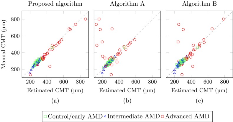
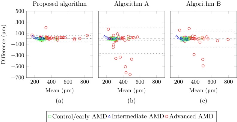
The average difference in CMT compared to the reference was 14.0 µm (± 22.1 µm) for the proposed algorithm and 42.9 µm (± 116.0 µm) and 27.1 µm (± 69.3 µm) for Algorithms A and B, respectively. Figure 12 shows the scatter plots indicating the reliability of the CMT measures derived from the proposed algorithm and Algorithms A and B, compared to the reference annotations. The corresponding Bland-Altman plots for each algorithm are shown in Fig. 13. The systematic difference between the manual CMT measures and the measures obtained by the proposed method is 7.0 µm with the 95% limits of agreement at −42.3 µm and 56.3 µm, for the lower and upper bound, respectively. The systematic difference for Algorithm A and B was −26.1 µm and −6.0 µm, respectively. The lower and upper bound of the 95% limits of agreement for Algorithm A were at −209.7 µm and 209.8 µm, and at −150.7 µm and 138.6 µm for Algorithm B.

Fig. 12.

Reliability analysis of the CMT measures obtained with (a) the proposed algorithm (b) Algorithm A and (c) Algorithm B, compared to the reference annotations. The different AMD subgroups are shown in a different color and symbol. The dashed line indicates no systematic difference.

Fig. 13.

Bland-Altman plot of the agreement between the manual central macular thickness (CMT) measures and the measures obtained with (a) the proposed algorithm, (b) Algorithm A and (c) Algorithm B. The different AMD subgroups are shown in a different color and symbol. The dotted lines indicate the bias and the 95% limits of agreement. The dashed line indicates the zero bias line.

The agreement between CMT values from the reference annotations and the estimated values obtained by the proposed method reached an ICC value of 0.974 (95% CI: 0.960 - 0.983), compared to the ICC values of 0.215 (95% CI: 0.026 - 0.392) and 0.744 (95% CI: 0.642 - 0.821) obtained using Algorithms A and B, respectively.

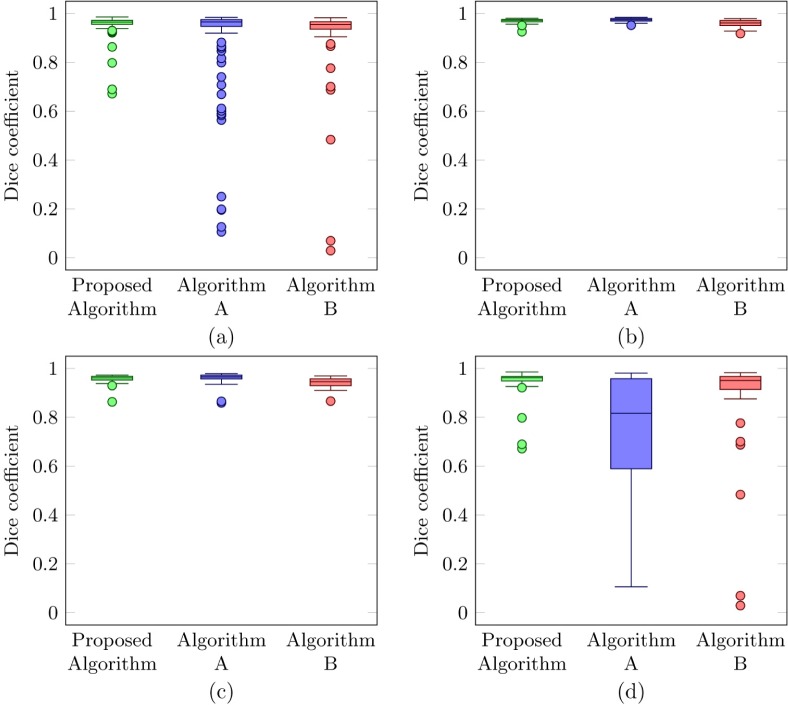
The average Dice-coefficient calculating the overlap between the segmented CMT area and the reference annotation was 0.954 (± 0.046) for the proposed algorithm, 0.887 (± 0.196) for algorithm A, and 0.920 (± 0.143) for algorithm B. Figure 14 shows the boxplots indicating the distribution of the dice coefficient from the proposed algorithm and Algorithms A and B, compared to the reference annotations.

Fig. 14.

Boxplots showing the distribution of the dice coefficient compared to the reference annotations (a) for all OCT volumes in the test set, (b) for OCT volumes with no pathology or signs of early AMD, (c) for OCT volumes with intermediate AMD, (d) for OCT volumes with advanced AMD.

The dice overlap coefficient obtained by the proposed method on the external set was 0.969 (± 0.005), while the Dice coefficient obtained by the method proposed in [32] was 0.985 (± 0.003). Human performance on this same dataset was 0.984 (± 0.002).

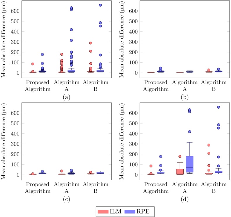
The mean absolute distance for the entire test set on an A-scan level for the proposed method was 6.8 µm (± 8.2 µm) and 18.2 µm (± 19.8 µm) for the ILM and RPE boundary respectively, whereas algorithm A obtained values of 16.9 µm (± 30.8 µm) and 56.9 µm (±125.6 µm), respectively. Algorithm B obtained a mean absolute distance of 16.4 µm (± 35.8 µm) for the ILM and 36.9 µm (± 92.4 µm) for the RPE. Figure 15 shows the boxplots indicating the distribution of the distance to the RPE and ILM boundary from the proposed algorithm and Algorithms A and B, compared to the reference annotations. Table 1 summarizes the mean CMT and the different error metrics compared to the reference annotations for the entire test set and for OCT volumes with different AMD severity levels.

Fig. 15.

Boxplots showing the distribution of the mean absolute distance from the ILM and RPE compared to the reference annotations (a) for all OCT volumes in the test set, (b) for OCT volumes with no pathology or signs of early AMD, (c) for OCT volumes with intermediate AMD, (d) for OCT volumes with advanced AMD.

Table 1.

Mean central macular thickness (CMT) and various errors metrics derived from the retina segmentation obtained with the different algorithms and compared to the reference annotations for the entire test set and for OCT volumes with different AMD severity levels.

	Reference annotation	Proposed algorithm	Algorithm A	Algorithm B
Overall
Mean CMT	321.4 ± 112.7 µm	328.4 ± 116.2 µm	295.4 78.0 µm	315.4 93.6 µm
Mean absolute CMT error	N/A	14.0 ± 22.1 µm	42.9 ±116.0 µm	27.1 ± 69.3 µm
Mean absolute distance to ILM	N/A	6.8 ± 8.2 µm	16.9 ± 30.8 µm	16.4 ± 35.8 µm
Mean absolute distance to RPE	N/A	18.2 ± 19.8 µm	56.9 ±125.6 µm	36.9 ± 92.4 µm
Mean Dice coefficient	N/A	0.954 ± 0.046	0.887 ± 0.196	0.920 ± 0.143
Early AMD
Mean CMT	288.3 ± 40.7 µm	282.3 ± 41.0 µm	287.2 ± 41.7 µm	287.6 43.2 µm
Mean absolute CMT error	N/A	8.2 ± 7.1 µm	6.5 ± 4.5 µm	9.4± 7.0 µm
Mean absolute distance to ILM	N/A	5.6 ± 1.2 µm	5.5 ± 1.1 µm	9.5 ± 4.4 µm
Mean absolute distance to RPE	N/A	14.1 ± 7.8 µm	9.5 ± 3.7 µm	13.6 ± 7.1 µm
Mean Dice coefficient	N/A	0.970 ± 0.010	0.973 ± 0.008 r	0.959 ± 0.014
Intermediate AMD
Mean CMT	266.0 ± 34.5 µm	272.5 ± 30.4 µm	269.9 29.2 µm	267.2 30.9 µm
Mean absolute CMT error	N/A	8.7 ± 8.1 µm	6.7± 7.9 µm	11.2± 9.7 µm
Mean absolute distance to ILM	N/A	5.6 ± 1.3 µm	6.7 ± 5.6 µm	10.1 ± 3.7 µm
Mean absolute distance to RPE	N/A	12.9 ± 4.7 µm	14.1 ± 7.5 µm	19.3 ± 8.1 µm
Mean Dice coefficient	N/A	0.957 ± 0.020	0.958 ± 0.027	0.942 ± 0.022
Advanced AMD
Mean CMT	409.1 ± 153.9 µm	430.5 ± 150.2 µm	329.0 118.8 µm	391.4 121.9 µm
Mean absolute CMT error	N/A	25.2 ± 34.5 µm	115.5 ± 181.6 µm	60.6 ± 113.2 µm
Mean absolute distance to ILM	N/A	9.2 ± 14.1 µm	39.4 ± 46.4 µm	30.3 ± 60.4 µm
Mean absolute distance to RPE	N/A	27.9 ± 31.5 µm	151.6 ± 188.4 µm	80.0 ±153.5 µm
Mean Dice coefficient	N/A	0.937 ± 0.075	0.721 ± 0.279	0.856 ± 0.237

The mean absolute distance from the ILM and RPE obtained by the proposed method on the external set was 5.0 µm (± 0.59 µm) and 6.3 µm (±1.3 µm), respectively. the method proposed in [32] obtained values of 4.7 µm (± 0.64 µm) and 4.95 µm (± 1.71 µm), for the ILM and RPE respectively. Human performance on this same dataset was 4.9 µm (± 0.8 µm) and 5.0 µm (±0.6 µm), for the ILM and RPE respectively.

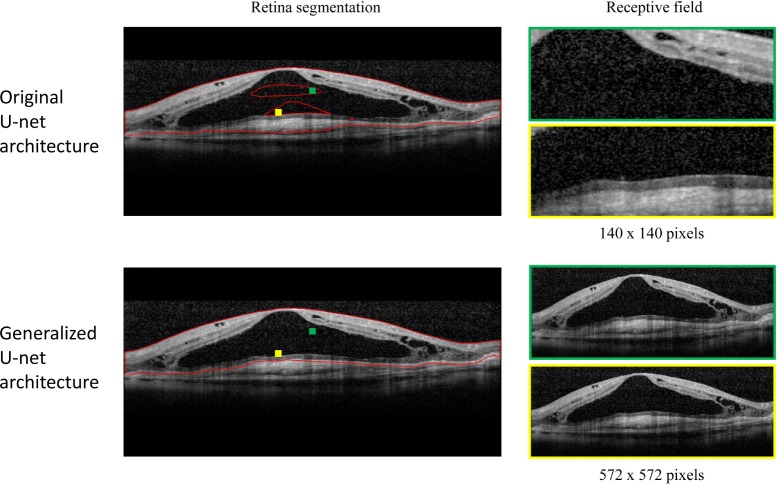
Figure 16(a) shows the Bland-Altman plot using the original U-net architecture instead of the proposed generalized architecture. The systematic difference for the original U-net architecture is 27.4 µm with the 95% limits of agreement at −52.1 µm and 106.9 µm, for the lower and upper bound, respectively. An example of the segmentation output obtained with the proposed architecture and the original U-net architecture is shown in Fig. 17.

Fig. 16.

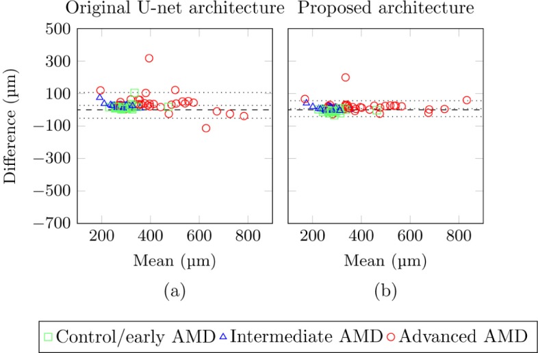
Bland-Altman plot of the agreement between the manual central macular thickness (CMT) measures and the measures obtained with (a) the original U-net architecture and (b) the proposed generalized architecture. The different AMD subgroups are shown in a different color and symbol. The dotted lines indicate the bias and the 95% limits of agreement. The dashed line indicates the zero bias line.

Fig. 17.

Effect of increasing the receptive field. Top: Original U-net architecture with a receptive field of 140 × 140 pixels, Bottom: Proposed generalized U-net architecture with a receptive field of 572 × 572 pixels. The red lines delimits the retina segmentation output obtained with each architecture. Examples of the receptive field used by each architecture for two different locations (highlighted in yellow and green boxes) are included. The receptive field for the generalized architecture is the entire image.

7. Discussion

In this work we developed and evaluated a CNN approach for retina segmentation in OCT volumes. A novelty of the developed system is its robustness and reliability in the presence of severe retinal pathology in which existing methods have been demonstrated to perform poorly [8].

Correct segmentation of the total retina in cases with severe pathology requires a segmentation algorithm that does not make too many assumptions about the structure and shape of the retina and takes a wide spatial context into account. The CNN architecture proposed in this work can fulfill both of these requirements. As opposed to fitting a segmentation boundary directly, the proposed algorithm performs a semantic segmentation where every pixel is classified as belonging to the retina or background. This indirect method of segmenting the retina adds the flexibility required to properly segment healthy retinas as well as pathological retinas. Moreover, as opposed to other pixel classification algorithms, the wide variability that can occur in the structure and shape of the retina is easily captured by the large number of free parameters that are present in a typical CNN. Another important aspect required to deal with large changes in the retina is the inclusion of spatially distant information in determining the probability of a pixel belonging to the retina. The hypo-reflective content of a fluid filled space (see Fig. 17) can easily be confused with the vitreous fluid or the choroidal tissue if only considering a small window around each pixel. The inclusion of a wide spatial context is achieved by using the generalized U-net architecture introduced in this work that is capable of providing a large receptive field while maintaining localization accuracy.

The original U-net provides a receptive field of 140×140 pixels [47], which is not large enough to cover the largest abnormalities present in our dataset. With this receptive field segmentation errors occurred for certain pixels inside large abnormalities as not enough contextual information was included to differentiate them from the vitreous fluid or the choroidal tissue. Figure 17 shows example segmentations for the original U-net and the proposed generalized architecture. It can be observed that for the original network with a receptive field of 140 × 140 segmentation errors occur inside the large fluid-filled abnormality. A possible explanation for these type of errors is that the top or bottom of the retina is not included in the receptive field, giving the network the impression that the pixel is part of the vitreous fluid or choroidal tissue, respectively. When increasing the receptive field further to 572 × 572 these type of errors did not occur anymore as the entire abnormality was included in the receptive field and enough contextual information was included to make a correct classification.

It has to be noted that recently introduced techniques like dropout [58] and batch normalization [59], that can be effective in preventing overfitting and can improve performance and convergence of the network, have not been used in the proposed architecture. The authors believe that the typical minor improvements in performance that these additions offer do not justify the additional complexity of the network architecture, and distract from the main contributions proposed in this work. A small increase in segmentation performance is therefore expected when adding techniques like drop-out and batch normalization.

The proposed algorithm was compared to two reference algorithms, one provided by a OCT camera manufacturer and the other widely used in research environments. These two algorithms are based on the segmentation of individual retinal layers to delimit the retina and obtain related measurements. Consequently, a large deviation in this layered structure, caused by for instance a fluid-filled space, often results in errors in the segmentation outputs obtained by these algorithms. A typical example of a severely disrupted retina and the segmentation boundaries for our algorithm and the two reference algorithms is shown in Fig. 9, where a large epithelial detachment and intraterinal cyst disrupt the typical organized layered structure and shape of the retina. The errors are typically large, with parts of the retina being excluded (see Fig. 9(c)) or even completely off (see Fig. 9(b)). Figure 9(a) shows a correct segmentation boundary produced by our proposed algorithm.

Figure 6(d) shows that these (large) errors are not incidental, but occurred regularly in OCT volumes with pathology present. For Algorithm A 78.8% of the segmentations contained such errors and were therefore rated as a failure by an experienced ophthalmologist. Algorithm B performs slightly better, but still 45.5% of the segmentations were rated as failure. Our algorithms improved dramatically upon these existing algorithms, with only 6.0% of the segmentations rated as failure. Moreover, the percentage of segmentations that is considered good was 66.7% for our proposed algorithm versus 6.1% and 18.1% for Algorithm A and Algorithm B, respectively.

When looking at the subgroups containing less severe pathology (Fig. 6(b) and Fig. 6(c)), the number of failures is decreased for both reference algorithms, but a substantial difference can still be observed compared to the proposed algorithm. Especially Algorithm B had surprisingly many failures in the easiest subgroup containing healthy controls and cases of early AMD (Fig. 6(b)). This is surprising as the structure of the retina, even in early AMD when only a few small drusen are present, is still largely intact. Visual inspection reveals that almost all errors could be attributed to cases where the RPE segmentation boundary makes a jump from the bottom of the RPE to the top of the RPE as shown in Fig. 7(c). The reason for this error is not entirely clear, but might be caused by the low B-scan density, ranging from 19 to 38 slices, of the OCT volumes used in this study. Algorithm B uses three-dimensional information to determine the segmentation boundaries, which makes sense for dense volumes as there is a strong correspondence between neighboring B-scans, but could cause problems in volumes with a low amount of B-scans due to the possible strong variation between consecutive B-scans.

Even though the proposed algorithm only had a single case rated as a failure in the subgroup of cases with intermediate AMD, 12 of the cases were rated as moderate (Fig. 6(c)). Upon visual inspection it turned out that the proposed algorithm tended to smooth out the small and intermediate drusen heavily present in intermediate AMD, resulting in a moderate rating for 12 cases. The reason for this under-segmentation may be caused by the under-representation of mild pathology in our training data. The performance of the proposed algorithm in this specific subgroup is expected to improve when adding more cases with intermediate AMD to the training data. Overall, the method proposed in this work can segment cases with a varying degree of pathology with a low rate of failure compared to existing methods as shown in (Fig. 6(a)).

To allow for comparison to other existing methods we evaluated the proposed algorithm on a publicly available dataset [32] and compared our results to the results obtained in the paper associated with the dataset. The algorithm could be applied without any modification and produced results close to human performance with a mean absolute distance of 5.0 µm (± 0.59 µm) to the ILM boundary compared to 4.9 µm (± 0.8 µm) for the human observer. The mean absolute distance to the RPE was 6.3 µm (± 1.3 µm) and 5.0 µm (± 0.6 µm) for the proposed algorithm and the human observer, respectively. Considering the proposed method was not trained using DME data, an increase in performance is expected when adding cases with DME to the training set. The algorithm published together with the public dataset obtained a mean absolute distance of 4.7 µm (± 0.64 µm) and 4.95 µm (± 1.71 µm) to the ILM and RPE boundary, respectively. For reference, a single pixel has an axial resolution of approximately 3.9 µm.

Robustness to severe pathology is an important and highly sought after feature in a retina segmentation algorithm, but application of an algorithm in practice also requires accurate segmentation boundaries and reliable clinical measures derived from it. When comparing the CMT produced by the proposed algorithm to annotations made by a human observer, a strong correlation (0.974) was found for the proposed algorithm compared to the two reference algorithms with correlation coefficients of 0.215 and 0.744 for Algorithm A and B, respectively. The reliability of the CMT measures was made more apparent in the scatter plots and Bland-Altman plots shown in Fig. 12 and Fig. 13. It can be observed in the scatter plots that less outliers are present for the proposed algorithm compared to the other algorithms. Moreover, the outliers that were present were all part of the subgroup containing cases with advanced AMD, indicating that the other 2 methods had trouble segmenting cases with more severe pathology. The more extreme outliers corresponded to the most severe failures where the segmentation boundaries were completely wrong, e.g. Fig. 9(b). As mentioned these type of errors occurred more frequently for Algorithm A.

The Bland-Altman plots showed a strong agreement for the proposed algorithm, indicated by the narrow 95% limits of agreement compared to the other two methods. The mean error over all cases in the test set for the proposed algorithm was 7.0 µm, indicating a small positive bias. The reference algorithms had a bias of −26.0 µm and −6.0 µm, for Algorithm A and Algorithm B respectively. Although the bias for Algorithm B was slightly smaller, the 95% limits of agreement were far larger compared to the proposed algorithm. Algorithm A, due to the earlier mentioned severe failures had very large 95% limits of agreement. As positive and negative segmentation errors cancel out, the absolute error gives a better indication of the typical size of the error that is made. The mean absolute error for Algorithm A is 42.9 µm, while Algorithm B has an error of 27.1 µm, the proposed algorithm has the lowest absolute error of 14.0 µm.

To conclude, the CNN introduced in this work has shown to be capable of modeling the wide variability in retinal appearance resulting in a robust retina segmentation even when severe pathology is present. Moreover, the method allows for reliable clinical measurements based on the retina segmentation such as CMT measurements. A robust segmentation algorithm that produces reliable clinical measurements is crucial when using the system in large clinical studies where manual verification and correction of the segmentation boundaries is undesirable or even unfeasible. Our automated system with performance in this range should therefore be considered a robust and reliable alternative for subjective and time-consuming manual measurements of retinal thickness in retinal research and clinical practice.

Funding

The author was supported by the following foundations: MD fonds, LSBS fonds and OOG fonds that contributed through UitZicht. The funding organizations had no role in the design or conduct of this research. They provided unrestricted grants.