

Abstract
We propose a unified Bayesian framework to detect both hyper- and hypo-active communities within whole-brain fMRI data. Specifically, our model identifies dense subgraphs that exhibit population-level differences in functional synchrony between a control and clinical group. We derive a variational EM algorithm to solve for the latent posterior distributions and parameter estimates, which subsequently inform us about the afflicted network topology. We demonstrate that our method provides valuable insights into the neural mechanisms underlying social dysfunction in autism, as verified by the Neurosynth meta-analytic database. In contrast, both univariate testing and community detection via recursive edge elimination fail to identify stable functional communities associated with the disorder.
Index Terms: Bayesian modeling, community detection, functional magnetic resonance imaging, population analysis
I. Introduction
UNIVARIATE analyses of fMRI activation patterns [1], [2] have allowed us to localize functional differences induced by neurological disorders, such as autism [3]–[5]. Despite the insights gained from univariate methods, there is increasing evidence that complex pathologies reflect distributed impairments across multiple brain systems [6]–[8]. These findings underscore the importance of network-based approaches for functional neuroimaging data.
The seminal works of [9]–[11] propose a series of large-scale network measures, which have precipitated the discovery of small-world functional architectures in the brain [12]. Disruptions of the small-world organization are believed to play a role in neurological disorders [13], [14]. However, these aggregate properties (e.g., small-worldness, centrality and degree distribution) do not illuminate concrete etiological mechanisms. Recently, more sophisticated models, based on directed Bayesian networks, have been proposed for fMRI data [15], [16]. Unfortunately, due to the large number of parameters, causal interactions are typically estimated on a restricted set of nodes. Moreover, these methods have difficulty estimating the directionality of connection information due to noise and subject differences. In contrast, we present a hierarchical framework that captures the underlying topology of the altered functional pathways. We extract both hyper- and hypo-active communities while simultaneously accommodating population variability.
Community detection is the process of identifying highly interconnected subgraphs within a larger network; these nodes (i.e., community members) share common properties and are crucial to understanding the organization of complex systems [17], [18]. Traditional community detection algorithms include hierarchical cluster analysis [19], which constructs an agglomerative dendrogram based on pairwise similarity measures, and spectral clustering [20], [21], which leverages higher-order network information in the Laplacian eigenvectors. Despite their prevalence, both methods fail to detect stable communities in noisy graphs, or when the clusters are significantly mixed [17], [22]. Recently, there has been a shift towards divisive algorithms, which identify and remove inter-cluster edges. The seminal work of [23] recursively eliminates network edges based on three centrality measures, and most importantly, recalculates the edge scores after each iteration. Similar approaches have been developed using modularity [24]–[26], clustering coefficient [27], and information compression [28] as selection criteria. While promising, the above methods are heuristic and do not assume a principled model of community structure [18].
Modularity-based approaches have recently been applied to fMRI data [29]–[31]. Broadly, the works of [29], [30] estimate a hierarchical community organization independently within each subject and use a post-hoc cluster matching procedure to perform group-level statistical analysis. Unfortunately, the results depend heavily on preselected thresholds and subroutines (i.e., adjacency matrix construction, subgraph alignment). Moreover, since these approaches do not impose topological constraints on the group differences, the clinical findings are difficult to interpret. The alternative method reported in [31] identifies statistical differences in betweenness centrality and average path length, neither of which informs us about the network structure and organization. In contrast, our model automatically identifies the abnormal networks with minimal user input.
Our approach goes beyond the prior literature in three crucial ways. First, we propose a unified generative model that describes the relationship between population templates and individual subject observations. Second, we perform community detection in the space of group-level functional differences, which allows us to identify both heightened and reduced synchrony. Finally, our framework can simultaneously detect multiple abnormal communities of varying type. We have previously used generative models to infer disease foci from resting-state fMRI data [32]–[34]. Our current framework identifies interconnected cliques within task fMRI data (different from an outward spreading model), and it distinguishes between hyper- and hypo-active subgraphs1. These two properties describe a fundamentally different network topology, which has not been captured by prior Bayesian models. While an early version of this work was presented in conference form [35], the present effort provides detailed derivations of the model and estimation procedure, along with more extensive experimental evaluation of the method.
We demonstrate our approach on an fMRI study of social perception in autism. Autism Spectrum Disorder (ASD) is characterized by impaired social-emotional reciprocity, communication deficits, and stereotyped behavior [36]. Furthermore, many individuals with ASD exhibit enhanced perception of detail, which is related to a sharper focus of spatial attention, or “tunnel vision” [37]. Despite ongoing efforts, the etiological complexity and acute heterogeneity of ASD has greatly limited our understanding of its pathogenesis. One prevailing theory posits that ASD alters the developmental trajectory of inter-regional connections [7], [38], [39]. Accordingly, task fMRI studies reveal both hyper- and hypo-connectivity between the prefrontal cortex, superior temporal sulcus and limbic structures [7], [4]. However, such analyses are restricted to predefined neural systems and do not reflect whole-brain information. Likewise, network approaches have detected group differences in node-based measures [40], [41] but have not illuminated a specific neural pathways for ASD. Our method provides valuable insights into ASD by extracting stable communities that reflect either heightened or reduced brain synchrony. These subnetworks map onto key functional domains, in which autistic individuals exhibit strengths and vulnerabilities, respectively. We demonstrate robustness or our results via bootstrapping and meta-analysis.
The remainder of this paper is organized as follows. We introduce our generative model in Section II and develop the corresponding inference algorithm in Section III. Section IV presents the methods used to empirically validate our framework. Sections V and VI report our experimental results based on synthetic and clinical data, respectively. Section VII discusses the behavior of our model, its advantages and drawbacks, and future directions of research. Finally, we conclude with a summary of contributions in Section VIII.
II. Generative Model of Abnormal Communities
Our graph representation assumes that each node is a region in the brain, and each edge describes the pairwise functional synchrony between nodes. The brain is partitioned into N regions based on a common atlas, which ensures that the region boundaries are consistently defined across subjects. Pairwise observations 〈i, j〉 are generated by correlating the fMRI signals in region i and region j. We assume that group-level functional differences can be represented by K interconnected subgraphs. In order to model both enhanced and impaired processes, we further stipulate that each subgraph reflects either a uniform increase or decrease relative to the neurotypical functional synchrony between regions. For simplicity, we assumes that the K networks are disjoint; this constraint helps us to infer multiple network influences.
Fig. 1 outlines our hierarchical Bayesian framework. The white boxes correspond to latent variables, which specify a template organization in the brain that we cannot directly access. Rather, we observe noisy measurements of the hidden structure via subject-wise fMRI correlations (shaded boxes), which are generated stochastically from the population-level latent structure. As seen, the K communities are grouped into subsets of regions based on the indicator variables {Ri}. Each network is associated with a binary label Yk that denotes either a hyper-active (Yk = 1) or a hypo-active (Yk = 0) subgraph. In this work Yk is specified a priori by the user for greater control over the results. This level of input is akin to setting the number of clusters or dictionary components in an unsupervised learning scenario, and it enables us to explore the network evolution in the absence of ground truth. If desired, it is straightforward to model Yk as an unknown Bernoulli random variable, as described in the Supplementary Materials.
Fig. 1.
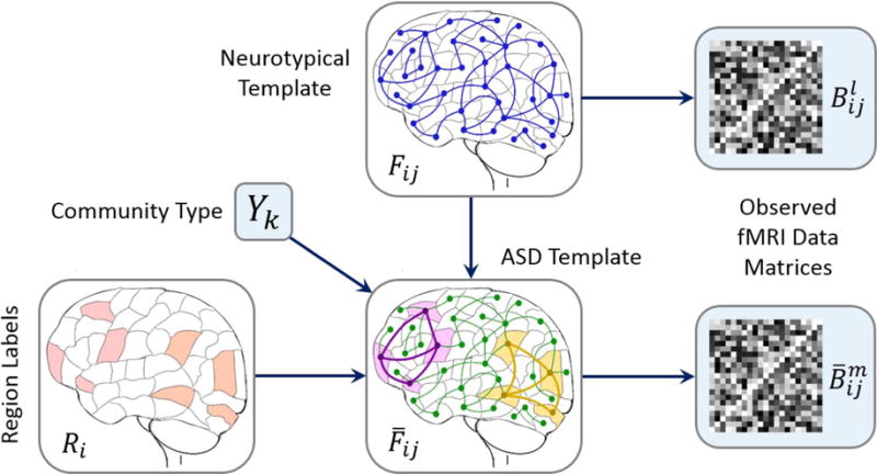
Hierarchical model of community structure for K = 2. The label Ri indicates whether region i is healthy (white) or whether it belongs to one of the two abnormal communities (red). The binary variable Yk denotes either a hyper-active (purple) or hypo-active (yellow) subgraph k. The neurotypical template {Fij} provides a baseline functional architecture for the brain, whereas the clinical template describes the latent organization of ASD. The green connections 〈i, j〉 are unchanged from baseline; the purple and yellow lines signify heightened and reduced synchrony, respectively. Each template generates a set of subject observations and for the group.
We use multinomial variables Fij and to denote the latent functional synchrony between regions i and j in the neurotypical and clincal groups, respectively. Empirically, we find that three states: low (Fij = 0), medium (Fij = 1), and high (Fij = 2), adequately capture the dynamic range and variability of our fMRI dataset. The conditional relationships are defined such that within a hyper-active community, and within a hypo-active community.
The fMRI metrics for subject l and for subject m are noisy observations of the underlying latent structure. Table I summarizes the random variables and nonrandom parameters in our generative model. Although the variable definitions are similar to [33], our current framework specifies a multi-cluster community organization. Below we formalize the mathematical representations.
Table I.
Random Variables (top) and Non-Random Parameters (Bottom) in our Graphical Model Shown in Fig. 1.
| Ri | Multinomial variable that indicates the state (healthy or belonging to community k) for each brain region i | |
| Fij | Latent functional connectivity between regions i and j in the neurotypical population | |
|
|
Latent functional connectivity between regions i and j in the clinical population | |
|
|
Observed fMRI correlation between regions i and j in subject l of the neurotypical population | |
|
|
Observed fMRI correlation between regions i and j in subject m of the clinical population | |
|
| ||
| πr | Prior for multinomial region indicator Ri (K+1 states) | |
| πf | Prior for multinomial functional connectivity Fij (3 states) | |
| η | Concentration of abnormal edges within the latent communities | |
| ε | Probability of deviating from the idealized graph of aberrant functional connectivity | |
| μs | Mean fMRI correlation given that Fij = s (s = 0, 1, 2) | |
|
|
Variance of fMRI correlation given that Fij = s (s = 0, 1, 2) | |
Node Selection
Let N represent the total number of regions in the brain. The multinomial random variable Ri (i = 1,…, N) indicates whether region is healthy (Ri = 0), or whether it belongs to an abnormal community k (Ri = k). We assume an i.i.d. multinomial prior for Rias follows:
| (1) |
The (K + 1) unknown parameters specify the a priori probabilities of a node assignment such that . Our model assumes that these values are shared by all regions.
Neurotypical Connectivity
The latent functional synchrony Fij denotes the co-activation between regions i and j in the neurotypical template. As previously described, Fij is modeled as a tri-state random variable. For notational convenience, we represent Fij as a length-three indicator vector, such that exactly one of its elements [Fij0 Fij1 Fij2]T is equal to one. The multinomial prior is i.i.d. across all pairwise connections, i.e.,
| (2) |
Abnormal Network Topology
The clinical variable in Fig. 1 is also tri-state; its value depends on the control template Fij and the abnormal communities defined by the region labels R and subgraph types Y. To derive the conditional distribution P( , R, Y), we first define an auxiliary graph {Tij}, which describes the idealized functional differences between member nodes of a community. Mathematically, Tij is a binary random variable that indicates either a healthy (Tij = 0) or an abnormal (Tij = 1) edge between nodes i and j:
| (3) |
Notice that the first case in (3) specifies the community organization of our abnormal subnetworks. Specifically, if regions i and j are not part of the same subnetwork (i.e., they have different labels or are both normal), then the corresponding functional edge is modeled as healthy (Tij = 0 deterministically). By extension, the functional edges that differ between groups must concentrate among member nodes of the same subnetwork; this defines a community topology.
On the flip side, when both regions are in the same community (i.e., Ri = Rj > 0), then we have two scenarios. First, the border conditions Yk = 1, Fij = 2 and Yk = 0, Fij = 0 represent hard constraints based on our variable definitions. Specifically, if Fij = 2, then cannot assume a higher state, as indicated by the community type Yk = 1, and likewise for the lower bound Fij = 0 and Yk = 0. In these cases, we assume that the latent functional synchrony is unaltered between the groups (i.e., Tij = 0). Alternatively, if the border conditions do not apply (last two cases), then Tij is Bernoulli with unknown parameter η. Notice that (3) is a special case of the planted ℓ-partition model [18], where η controls the density of edges within the abnormal communities.
Ideally, for healthy edges. However, if Tij = 1, then for Yk = 1, and for Yk = 0. However, to accommodate the complexities of fMRI data, we introduce a second level of noise, in which the scalar parameter ε controls the probability of deviating from the above rules. We marginalize the graph {Tij} to better estimate the community assignments Ri. Beginning with the first condition in (3), if regions i and j are not in the same community, then Tij = 0 and we obtain the following baseline distribution:
| (4) |
such that if the functional synchrony is the same between groups, and otherwise.
The conditional relationships between community members (i.e., Ri = Rj > 0) are given in Table II. Due to the distinction between hyper- and hypo-synchronous connections, the overall distribution cannot be represented compactly, as in our previous works [33], [42]. In practice, we expect the latent noise to be small (ε < 0.5) and the edge density to be moderate (0.4 < η < 0.6). Hence, the largest entries in Table II will involve the term 1 – ε. Notice that this term appears in the upper quadrant (i.e., ) for the hyper-active case and in the lower quadrant (i.e., ) for the hypo-active case. For notational convenience, we denote entries of Table II as , where Fij = s, , and Yk ∈ {1, 0}, for the top and bottom sub-tables.
Table II.
Conditional Distribution P( , R, Y; η, ε) for Hyper-Active (top) and Hypo-Active (Bottom) Communities.
| Ri = Rj = k > 0 and Yk = 1 | |||||||
|
|
|||||||
| 0 | 1 | 2 | |||||
| Fij | 0 | (1 − η)(1 − ε) + ηε |
|
|
|||
| 1 | ε/2 | (1 − η) (1 − ε) + η(ε/2) | (1 − η)(ε/2) + η(1 − ε) | ||||
| 2 | ε/2 | ε/2 | 1 − ε | ||||
| Ri = Rj = k > 0 and Yk = 0 | |||||||
|
|
|||||||
| 0 | 1 | 2 | |||||
| Fij | 0 | 1 − ε | ε/2 | ε/2 | |||
| 1 | (1 − η) (ε/2) + η(1 − ε) | (1 − η)(1 − ε) + η(ε/2) | ε/2 | ||||
| 2 |
|
|
(1 − η)(1 − ε) + ηε | ||||
Data Likelihood
The fMRI correlation between regions i and j in neurotypical subject l is a noisy realization of the latent functional template Fij. We assume a gaussian distribution, with mean and variance controlled by Fij:
| (5) |
The likelihood for a clinical patient has the same functional form as (5) but relies on the clinical template . We compute via pearson correlation coefficients. Our prior work [42] has demonstrated that Gaussian distributions can adequately capture the global fMRI statistics, while greatly simplifying the parameter estimation steps.
III. Model Inference
Given the observed fMRI measurements , we employ a maximum likelihood (ML) framework to fit our hierarchical Bayesian model to the data. Let Θ = {πr, πf, η, ε, μ, σ2} denote the collection of non-random model parameters, and let L and M be the number of subjects in the neurotypical and clinical populations, respectively. For convenience, we now switch to a binary vector representation for the region labels Ri. Specifically, Ri = [Ri0 Ri1…RiK]T, such that the state Ri = k implies that Rik = 1 and the remaining entries are equal zero.
Combining the distributions in (1)–(5) with the expressions in Table II yields the following joint density for the latent and observed random variables:
| (6) |
We observe that the community structure is specified by the third and fourth lines of (6), which denote the natural logarithm of the baseline distribution in (4). Also, while (6) assumes that the subgraph types {Yk} are given, the contribution of Yk in lines 5–6 is equivalent to that of a Bernoulli random variable. Therefore, by adding an i.i.d. Bernoulli prior: log P(Yk; πy) = Yk log(πy) + (1 − Yk) log(1 − πy), we can model these values as unknown. The incremental changes to our model are presented in the Supplementary Materials.
The community assignments Ri induce a complex coupling across pairwise connections 〈i, j〉. Therefore, we adopt a variational approximation [43] to infer the latent posterior distribution Q(·) and corresponding parameters , which minimize the variational free energy
| (7) |
Notice that the quantity is a lower bound to the marginal log-likelihood P(X|Y; Θ) in the original ML framework.
Our approximate posterior assumes the factorized form:
| (8) |
As seen, is a multinomial distribution with K + 1 states, parameterized by . Likewise, is a multinomial distribution with 9 states, parameterized by , which account for the 9 configurations in Table II. Essentially, is the posterior probability that Ri = k, and is the posterior probability that Fij = s and . The factorization in (8) preserves the region-to-connection dependencies and is scalable to accommodate a large number of parcels N.
Using (8), we can expand the entropy term ℋ(Q) in (7) as shown below:
| (9) |
The expectation with respect to Q(·)of the complete log-likelihood shares the same form as (6), but with the following substitutions:
In the next section, we describe a coordinate descent algorithm to estimate both the parameters of the variational posterior and the nonrandom model parameters Θ.
A. Variational EM Algorithm
1) E-Step
For a fixed setting of model parameters , we iteratively update the elements of Qr(·) and Qc(·) to minimize the variational free energy. The iterations for can be expressed in closed form given :
| (10) |
where the proportionality constant is computed such that . The first three lines in (10) leverage the prior and latent functional interactions, whereas the last line incorporates the data likelihood for both populations.
In contrast, differentiating with respect to results in coupled update expressions
| (11) |
Since (11) depends on the other region posterior estimates , we perform an inner fixed-point iteration until convergence of the distribution Qr (R).
The estimates for Θ in the following section rely on marginal probabilities of . We compute these quantities after convergence of the full variational posterior:
| (12) |
| (13) |
2) M-Step
We update the model parameters by fixing the posterior distribution Q(R, F, ) and setting the gradient of (7) with respect to equal to zero. The expressions for the multinomial prior parameters {πr, πf} reduce to averages over the marginal posterior distributions:
| (14) |
| (15) |
where C = N (N − 1)/2 is the total number of unique pairwise connections between N regions.
The fMRI likelihood parameters are estimated as weighted statistics of the data. The updates parallel those of a standard Gaussian mixture model:
| (16) |
| (17) |
We jointly update the edge concentration η and latent noise ε via Newton’s method. Details of this step are presented in the Supplementary Materials. We emphasize that given the community types Y, both the posterior distribution and the model parameters are estimated directly from the observed data. We do not tune any auxiliary parameters or thresholds.
B. Initialization
Like many gradient-based methods, the final solution to our model will depend on proper initialization. At a minimum, the variational EM algorithm in Section III-A requires us to initialize the non-random model parameters and the region posterior variables . The algorithm proceeds by updating the connectivity posteriors in the E-step and iterating between the distributions until convergence. We then estimate the parameters in the M-step and repeat the outer loop.
We initialize the functional prior πf and the Gaussian means μ and variances σ2 based on statistics of the data. For regularization, we opt to center the correlation distributions of each subject and fix μ1 = 0 in subsequent analysis. This procedure effectively models the relative deviations from the baseline functional synchrony for each subject. We set the initial latent noise parameter to ε = 0.01, which encourages consistency between the region labels and the observed fMRI data, and we uniformly sample the edge concentration η from the interval [0.2, 0.5]. Larger values of η encourage more abnormal functional edges between community members. Likewise, we randomly initialize the region prior as πr = [(1−α) (α/K) … (α/K)]T, such that α ∈ [0.2, 0.5]. As α increases, the algorithm is biased towards larger communities during the first iteration.
Finally, we initialize the region posterior parameters via a two step procedure. First, we average the fMRI correlations across subjects and cluster these values to approximate the discrete latent functional connectivity. Second, we separate the hyper- and hypo-synchronous connections and apply a clique detection algorithm to each grouping. The initial communities are based on the regions associated with largest interconnected cliques. In practice, the initial communities consist of 4–6 regions, which is significantly less than in the final solution.
We mitigate the influence of local minima by randomly initializing the variational EM algorithm 10 times and select the optimal solution. This procedure is applied to both synthetic and real-world experiments.
IV. Model Evaluation
A. Estimating the Abnormal Network Topology
The idealized graph of functional differences {Tij} provides valuable insights into the topological properties of each abnormal community by removing the effects of the latent noise ε. Tij also describes the subset of community edges that strongly differ between the control and clinical populations.
We can retrospectively approximate these variables based on the maximum a posteriori (MAP) solution for R and the parameter estimates . Specifically, given R and Y, our model decouples by pairwise connection, so we can assign each Tij independently. Furthermore, (3) implies that Tij = 0 for Ri ≠ Rj and Ri = Rj = 0 (i.e., when the nodes belong to different communities and when they are healthy, respectively). For the remaining case (Ri = Rj > 0), we select the value Tij ∈ {0, 1} according to the following optimization:
| (18) |
The right-hand side of (18) can be computed by multiplying the natural logarithm of entries in Table II with the corresponding variational posterior parameter and summing across all nine configurations of {Fij, }. This computation weighs the influence of the edge density η, which controls the proportion of abnormal connections, against the latent noise ε, which encourages the functional templates to deviate from the rules outlined in (3).
B. Robustness of the Identified Communities
The marginal posterior statistics inform us whether region i is healthy or if it belongs to one of the K abnormal communities. We evaluate the robustness of these region assignments via bootstrapping. In particular, we fit the model to random subsets of the data, such that the ratio of neurotypical controls to ASD patients is preserved. Each subset contains only 80% of the total number subjects. We re-sample the data subsets 50 times and average the estimated posterior across runs to quantify the influence of region i.
We focus on region stability for three reasons. First, due to the community organization built into our model, abnormal edges are constrained to lie between member nodes of the same subnetwork. Moreover, the sign of each edge (i.e., hyper- vs. hypo-synchronous) is given by the binary vector Y. Therefore, the topology of the group-level functional differences is largely specified by just the region assignments and community types. Second, the bulk of our knowledge about the brain is organized around regions (i.e., functional localization, tissue properties, morphometry) and not the connections between them. From a clinical perspective, we can use the region assignments to perform follow-up analyses (see Neurosynth below); but the connectivity pattern is much harder to interpret. Finally, our previous work [33], [44] suggests that connection-wise differences may not be as robust as region measures.
C. Baseline Methods
We compare our generative model with two alternative techniques: statistical testing and a well-known community detection procedure, which prunes edges from the original network. These comparisons evaluate the benefits of (1) an imposed community organization, and (2) explicitly differentiating between hyper- and hypo-active communities.
Univariate testing is one of the standard approaches used in population studies of functional connectivity. Specifically, the two sample t-test confirms or rejects the null hypothesis that the group means of a given fMRI correlation are equal. Here, we vary the significance threshold in order to determine whether univariate functional differences naturally exhibit an underlying community structure.
Our second comparison implements the seminal method of [23], which iteratively removes edges from the network in order to discover community structure. The edges are selected according to a current-flow betweenness measure, which favors connections that lie between communities rather than ones that span a single community. This procedure requires a sparse binary input graph A that describes the group-wise functional differences. Rather than averaging and thresholding the fMRI correlation values, we construct A via the Bayesian connection model described in [42]. Specifically, Aij = 1 if the posterior probability that the latent functional connectivity templates differ exceeds 0.5. We take this approach because data thresholding introduces nonlinear dependencies into the analysis, which are known to bias network results [45]. Moreover, since the fMRI likelihood in [42] is the same as (5), we can directly evaluate the gain from our community priors.
D. Meta-Analysis via Neurosynth
The Neurosynth database (www.neurosynth.org) provides an unbiased and comprehensive evaluation of the functionality supported by each hyper- and hypo-active community. Specifically, the database aggregates both the MNI activation coordinates reported in prior fMRI studies along with a set of descriptive words and phrases pulled from the abstracts. The meta-analytic framework leverages the power of large datasets to calculate the posterior probability P(Feature|Coordinate) for an individual psychological feature (i.e., word or phrase) at a given spatial location [46]. Essentially, this reverse inference procedure identifies psychological constructs that have consistently been associated with a particular activation coordinate across a range of fMRI studies (varying paradigms, demographics and clinical statuses). Neurosynth has precomputed and stored 3,099 brain maps based on this posterior information; each map is associated with a given feature term. Additionally, the website creators have used Latent Dirichlet Allocation (LDA) [47] to identify a set of high-level topics from the original 3,099 words and phrases.
In this work, we correlate the spatial regions defined by each hyper- and hypo-active community with the statistical maps stored in the Neurosynth database; terms with a correlation above the default threshold (r > 0.001) were retained. We then apply the methods of [46], [48] to perform a whole-brain reverse inference for each LDA topic and rank them according to their association with each abnormal community.
V. Results on Synthetic Data
In this section, we use simulated experiments to demonstrate that our variational EM algorithm recovers the ground truth region labels. We assume group differences can be explained by one hyper-active and one hypo-active community (K = 2). Subject correlations are generated according to Fig. 1 for different noise statistics and community organizations.
A. Experiment I: Preliminary Evaluation
As a baseline, we first generate subject observations using the same signal-to-noise ratio and community properties estimated by the maximum likelihood solution of our clinical dataset. In particular, we set (μ1 – μ0) = 0.13, (μ2 – μ1) = 0.2, and for the data likelihood. Notice that there is significant overlap in the correlation distributions for the three latent connectivity states, i.e, the standard deviation of each Gaussian is 2–3 times greater than the separation between the means. We mimic the organization of our clinical dataset by specifying an underlying network with 150 regions and sampling 50 subjects in each population. The latent concentration and noise parameters are fixed at η = 0.5 and ε = 0.03.
During each trial, we uniformly sample the region prior πr such that 11–16% of regions belong to each abnormal cluster. We generate the latent variables in the following order , and we use the variational EM algorithm to infer the region posterior statistics . Fig. 2 (left) illustrates the average errors across 50 random trials. As seen, the probability of a false alarm or wrong assignment is negligible. While the probability of a missed detection is slightly higher, the median error is only 7%, and the 75th percentile error is under 9%. Fig. 2 (right) suggests an inverse relationship between the detection error and the minimum community size. Intuitively, larger communities have more abnormal edges and are easier to identify, whereas smaller communities are more likely to be overwhelmed by noise.
Fig. 2.
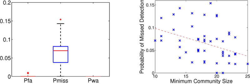
Results of Experiment I across 50 synthetic trials. Left: Errors in region assignment corresponding to the probability of false alarm (Pfa), the probability of a miss (Pmiss) and the probability of an abnormal region being assigned to the wrong community (Pwa). Right: Inverse relationship between Pmiss and the minimum community size.
B. Experiment II: Effect of Community Organization
Next, we evaluate the sensitivity and robustness of our algorithm with respect to the edge concentration η and the latent noise ε. We expect the region assignment errors to be positively correlated with ε and negatively correlated with η. This is because higher values of η increase the density of abnormal connections within each community, thus making them more distinctive. Conversely, larger ε results in more functional connections deviating from the ideal community organization (i.e., Tij). Here, we present only the probability of a missed detection.
We sweep the parameters of interest across the range η ∈ [0.1, 1] and ε ∈ [0.01, 0.1] in increments of 0.1 and 0.01, respectively. For each (η, ε) pair, we generate the latent variables and observed data as described in Section V-A. Once again, the region prior πr is sampled such that 11–16% of region belong to each community. We consider two likelihood parameterizations {μ, σ2}. The Good Data parameterization clearly separates the data distributions for each latent functional state. Specifically, we set (μ1 – μ0) = (μ2 – μ1) = 0.35 and for s = 0, 1, 2. This configuration allows us to accurately infer the latent templates {F, }, which are then used to delineate abnormal communities. The Noisy Data parameterization uses the same likelihoods as Section V-A.
Figs. 3 and 4 report the proportion of missed community nodes (Type I error) across 50 synthetic trials for the Good data and Noisy Data parameterizations, respectively. These results highlight three particularly striking trends. First, the performance of our model and algorithm worsens with increasing ε. Intuitively, ε controls the proportion of both missing and spurious connections within the multi-class community organization, which hinders our ability to identify the abnormal subnetworks. Second, in accordance with our initial hypothesis, there is an inverse relationship between the concentration η and the Type I error, with an inflection point at η = 0.5. The parameter η controls the percentage of nonzero edges between community members and is closely linked to the probability pin from the planted ℓ-partition model [49]. Hence, our model can only extract dense subgraphs. Finally, we observe that the error rates are similar for both likelihood parameterizations. This suggests that errors in community detection are primarily due to inconsistent functional differences rather than to noisy data observations.
Fig. 3.
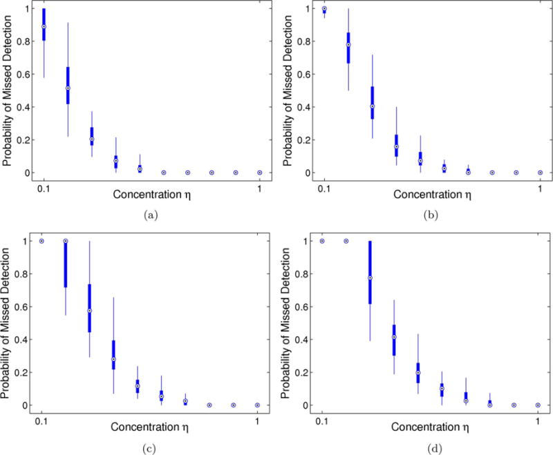
Probability of missed detection (Type I error) for the Good Data parameterization across 50 random samplings of the observed data. Thick lines correspond to the interquartile interval, and the whiskers extend to the 10–90% range. (a) Latent noise ε = 0.01 (b) Latent noise ε = 0.04 (c) Latent noise ε = 0.07 (d) Latent noise ε = 0.10.
Fig. 4.
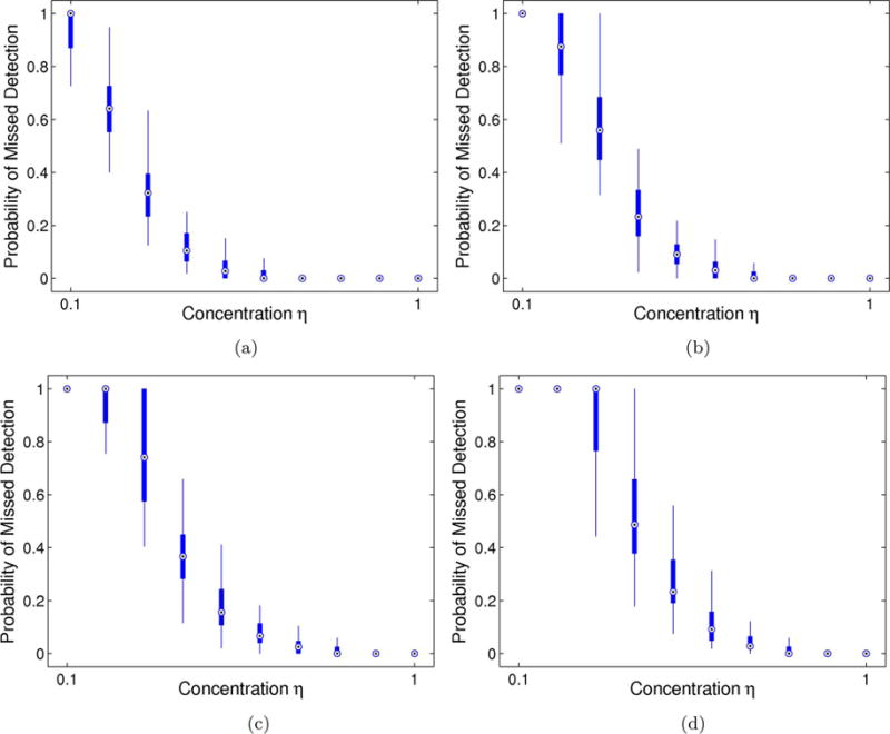
Probability of missed detection (Type I error) for the Noisy Data parameterization across 50 random samplings of the observed data. Thick lines correspond to the interquartile interval, and the whiskers extend to the 10–90% range. (a) Latent noise ε = 0.01 (b) Latent noise ε = 0.04 (c) Latent noise ε = 0.07 (d) Latent noise ε = 0.10.
VI. Social Perception in Autism
A. Biopoint Dataset and FMRI Preprocessing
We demonstrate our methods on a clinical study of 72 ASD children and 43 age-matched (p > 0.124) and IQ-matched (p > 0.122) neurotypical controls. For each subject, a T1-weighted scan (MPRAGE, TR = 1900 ms, TE = 2.96 ms, flip angle = 9°, res = 1 mm3) and a task fMRI scan (BOLD, TR = 2000 ms, TE = 25 ms, flip angle 60°, res = 3.44 × 3.44 × 4 mm, 164 volumes) were acquired on a Siemens MAGNETOM Trio TIM 3T scanner.
The experimental paradigm features coherent and scrambled point-light animations created from motion capture data. The coherent biological motion depicts an adult male actor performing movements relevant to early childhood experiences [50]. The scrambled animations combine the trajectories of 16 randomly selected points from the coherent displays. Snapshots of these stimuli are illustrated in Fig. 5. Six biological motion clips and six scrambled motion clips were presented in an alternating-block design (24s per block).
Fig. 5.
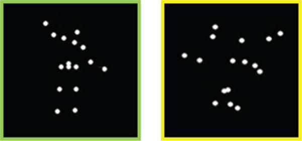
Snapshot of the visual stimuli. The protocol alternates between coherent biological motion (left) and scrambled animations (right).
We segment the anatomical images into 150 cortical and subcortical regions based on the Destrieux atlas in Freesurfer [51]. The fMRI data was preprocessed using FSL [52]. The pipeline was developed at Yale and consists of: 1) motion correction using MCFLIRT, 2) interleaved slice timing correction, 3) BET brain extraction, 4) spatial smoothing with FWHM 5mm, and 5) high-pass temporal filtering. The functional and anatomical data were registered to the MNI152 standard brain. The fMRI measure is computed as the Pearson correlation coefficient between the mean time courses of regions i and j. As previously stated, we center the correlation distribution of each subject and fix the likelihood mean μ1 during the model estimation procedure.
B. Abnormal Communities
We vary the number and type of communities Yk to explore the evolution of abnormal subnetworks. Recall that these subgraphs reflect atypical functional synchrony across the entire stimulus paradigm. Figs. 6 and 7 illustrates the community-based differences inferred by our model for K = 1 and K > 1, respectively. Table III reports the corresponding ML parameter values estimated by the variational EM algorithm.
Fig. 6.
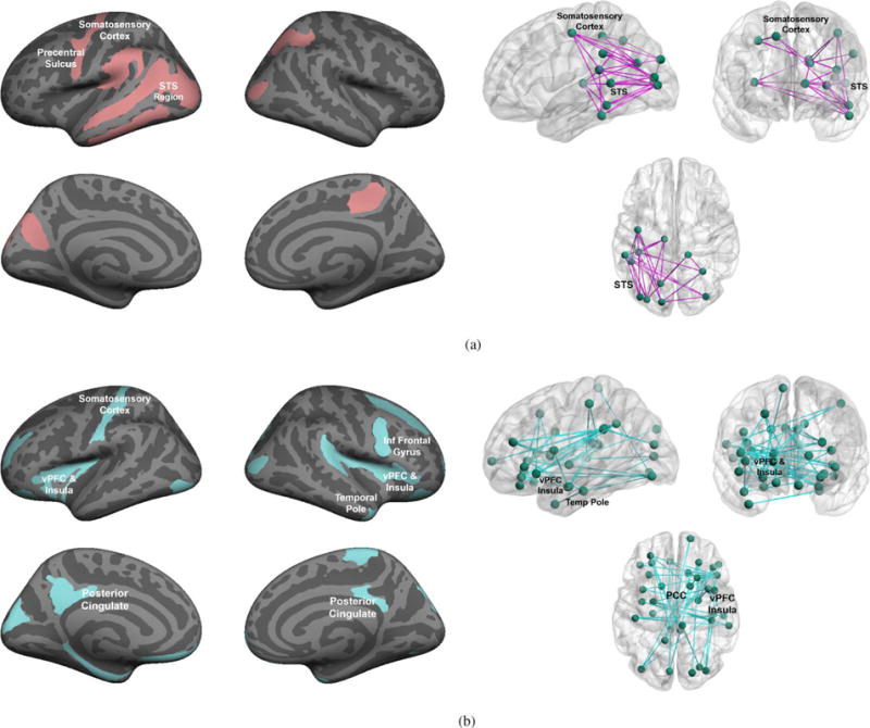
Abnormal communities inferred by our Bayesian model for K = 1. Left: Region membership in each community. Red nodes indicate the hyper-active community, whereas blue areas delineate the hypo-active cluster. Right: Estimated network of abnormal functional synchrony. Each node corresponds to one of the predefined regions, and each edge represents an abnormal functional connection between two community members. Blue lines signify reduced functional synchrony in ASD across the paradigm; magenta lines denote increased functional synchrony in ASD. (a) Hyper-active community: Y1 = 1 (b) Hypo-active community: Y1 = 0.
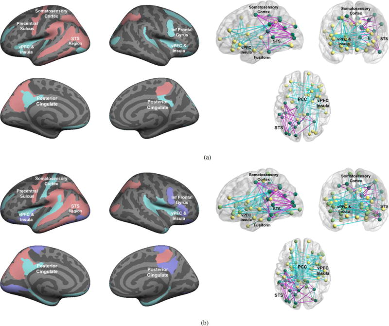
Fig. 7.
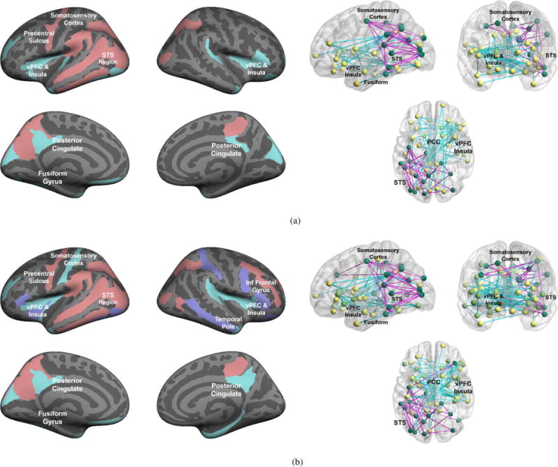
Abnormal communities inferred by our Bayesian model for K = 2 (top) and K = 3 (bottom). Left: Region membership in each community. Red nodes indicate the hyper-active community, whereas blue areas delineate the hypo-active cluster. Right: Estimated network of abnormal functional synchrony. Each node corresponds to one of the predefined regions, and each edge represents an abnormal functional connection between two community members. Blue lines signify reduced functional synchrony in ASD across the paradigm; magenta lines denote increased functional synchrony in ASD. (a) One hyper- and one hypo-active community: Y1 = 1 and Y2 = 0 (b) One hyper-active and two hypo-active communities: Y1 = 1 and Y2 = Y3 = 0.
Table III.
Latent Community Parameters (top) and Data Likelihood (Bottom), Estimated by the ML Solution for the Clinical Data.
|
|
|
|
|
|
|
η | ε | μ0 | μl | μ2 |
|
|
|
||||||||||
|---|---|---|---|---|---|---|---|---|---|---|---|---|---|---|---|---|---|---|---|---|---|---|---|
|
| |||||||||||||||||||||||
| Y1 = 1 | 0.094 | — | — | 0.34 | 0.44 | 0.22 | 0.65 | 0.041 | −0.13 | 0 | 0.19 | 0.072 | 0.062 | 0.058 | |||||||||
| Y1 = 0 | 0.25 | — | — | 0.34 | 0.44 | 0.22 | 0.45 | 0.034 | −0.13 | 0 | 0.19 | 0.072 | 0.062 | 0.059 | |||||||||
| Y1 = 1, Y2 = 0 | 0.11 | 0.22 | — | 0.34 | 0.44 | 0.22 | 0.54 | 0.031 | −0.13 | 0 | 0.19 | 0.072 | 0.062 | 0.059 | |||||||||
| Y1 = 1, Y2 = Y3 = 0 | 0.12 | 0.11 | 0.18 | 0.34 | 0.44 | 0.22 | 0.52 | 0.029 | −0.13 | 0 | 0.19 | 0.072 | 0.062 | 0.059 | |||||||||
Encouragingly, we observe a steady progression with the number of communities K in Figs. 6 and 7. In particular, as K increases, our model augments the previous community organization with an additional subnetwork of the required type. Similarly, the functional prior πf and data likelihood parameters {μ, σ2} in Table III are identical between model realizations. Differences in community organization seem to be captured by the region prior πr, the edge concentration η, and the noise level ε. This behavior indicates stability of the inferred latent functional templates, which are subsequently used to identify the abnormal communities. Further, these nested solutions provide empirical evidence for the validity of our model and inference algorithm.
Clinically, the hyper-active communities are depicted in red/pink and concentrate in the left superior temporal sulcus (STS), the visual cortex, and the somatosesory cortex. Conversely, the blue regions indicate hypo-activity. As seen, they localize to the bilateral ventral prefrontal cortex (vPFC), insula, and posterior cingulate. The hypo-active networks also includes subcortical activations in the caudate and amgydala, which are not shown on the cortical surface plots. The corresponding network diagrams [53] reveal increased synchrony between temporal and occipital nodes (magenta lines), along with reduced synchrony between the frontal and parietal nodes (blue lines). These results support a view of impaired social communication in ASD. Consistent with neurocognitive findings, Figs. 6 and 7 suggest hyper-connectivity, and perhaps hyper-functionality, in a visual perception network. Hypo-active circuits include two networks that are well known for their role in social cognition and the high-level interpretation of social stimuli [6], [7], [4].
C. Model Robustness
Figs. 8 and 9 report the average posterior probability of each region across 50 resamplings of the data for K = 2 and 3. We display only the regions for which , thereby emphasizing the most prominent patterns.
Fig. 8.
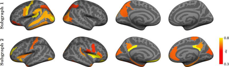
Average marginal posterior probability for each of the K = 2 communities across 50 random samplings of the fMRI data. Each sample includes 80% of the subjects, such that the ratio of ASD patients to neurotypical controls is preserved. The colorbar denotes the average posterior probability for each region i and community k.
Fig. 9.
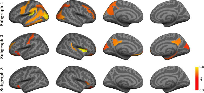
Average marginal posterior probability for each of the K = 3 communities across 50 random samplings of the fMRI data. Each sample includes 80% of the subjects, such that the ratio of ASD patients to neurotypical controls is preserved. The colorbar denotes the average posterior probability for each region i and community k. The clusters are aligned to the final solution in Fig. 7 to maintain correspondence of Yk.
Favorably, our bootstrapping analysis in Fig. 8 consistently recovers both the red hyper-active and blue hypo-active communities in Fig. 7(a). Additionally, subgraph 2 in Fig. 8 uncovers medial activations in the right hemisphere that are not present in the full solution. This behavior suggests that while some regions are weakly implicated by the data, they are not included in the full variational EM solution. Despite the inconsistency, reproducibility across 80% subsets has not been demonstrated in prior fMRI studies of ASD. Instead, prior works employ leave-one-out techniques, which artificially impose a stronger bias between samples.
The K = 3 model in Fig. 9 is able to recover the hyper-active community (Subgraph 1) with the same frequency as in Fig. 8. However, the reproducibility of the two hypo-active networks is much lower. Empirically, we observe that the nodes are shuffled between communities during the bootstrapping experiment, which reduces the overall consistency between trials. At the same time, highly-implicated regions, such as the posterior cingulate and insula, manage to survive our selection criterion. We note that the weakened robustness for K > 2 provides an important direction for future refinements to our model and inference algorithm.
D. Baseline Comparison
Figs. 10 and 11 illustrate the connectivity differences based on the two sample t-tests and the current-flow betweenness algorithm, respectively. For ease of visualization, we have colored each pairwise connection such that blue corresponds to reduced synchrony in ASD, and magenta denotes increased synchrony in ASD. However, we do not differentiate between heightened and reduced connections when applying the baseline methods. Hence, these results underscore the importance of our multi-cluster region labels and the community types Yk.
Fig. 10.
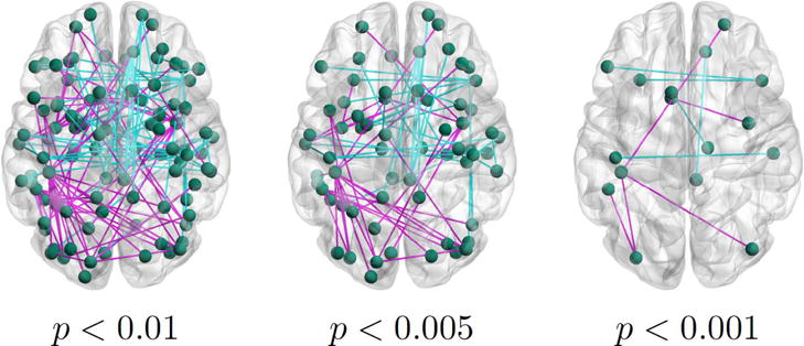
Population differences in functional connectivity when varying the significance threshold. Blue lines denote a lower average correlation across ASD patient than for neurotypical controls. Magenta lines signify the opposite relationship.
Fig. 11.
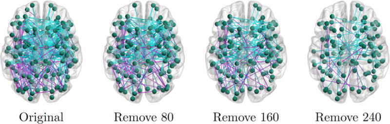
Community detection based on current-flow betweenness. Left to right depicts the original network of pairwise functional differences (294 edges) and the iterative removal of 80, 160 and 240 edges. Blue and magenta lines correspond to reduced and increased functional synchrony in ASD, respectively.
In Fig. 10 we threshold the (uncorrected) p-value to enforce different levels of statistical significance. As an aside, none of the connections survive a false discovery rate (FDR) correction for multiple comparisons, which suggests that the univariate functional differences are relatively weak in our dataset. Similar to Fig. 7, we observe interconnected magenta lines in STS region and a high concentration of blue lines in the default mode and precentral cortices for p < 0.01. There is also a second magenta cluster in the left frontal regions. Reducing the threshold to p < 0.005 prunes some of the connections; however, the frontal areas no longer exhibit a clique-like organization. Finally, the result for p < 0.001 contains isolated groups of vertices rather than a unified network.
The community detection procedure was applied to an original network of 294 edges, which corresponds to connection-wise latent functional differences, as computed via [42]. We notice that the initial graph is a superset of the connections identified by our model in Figs. 6 and 7. However, pruning the edges according to the current-flow betweenness measure does not reveal interconnected communities. For example, despite removing 80% of the edges in the rightmost figure, the overall number of nodes is fairly similar to the original network. Consequently, we cannot identify a natural stopping point for the algorithm. The observed behavior suggests that pairwise betweenness measures are insufficient to distinguish the core subnetworks associated with ASD.
E. Neurosynth Results
The polar plots in Fig. 12 illustrates the top nine meta-analytic constructs implied by the regions in each community, as inferred by our generative model. Recall that these topics reflect unbiased, aggregate findings across the fMRI literature. The functional dimensions in Fig. 12 expose a clear functional distinction between the two community types. Specifically, the hyper-active network maps onto visual perception and pattern recognition domains for both K = 2 and K = 3. Correspondingly, individuals with ASD tend to outperform their neurotypical peers in such tasks [54]. In contrast, the hypo-active networks implicate areas of clear deficit in ASD, such as emotion regulation and social communication, perception and reward. There is also considerable overlap in the functionality of the blue and green networks in Fig. 12(b), likely driven by community membership of the bilateral STS, vPFC and insulae. At a high level, our Neurosynth results support the hypothesis that ASD children are more stimulated by the point-light animations but are failing to grasp the social context. This conclusion fits nicely both with behavioral observations when administering the fMRI paradigm, and with a prevailing theory that ASD includes areas of cognitive strengths amidst the social deficits [37], [55], [56].
Fig. 12.
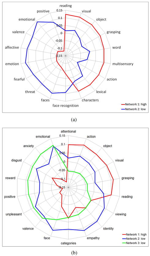
Correlation values of the top 9 features for each network based on the Neurosynth database. These topics represent the specificity of neurocognitive functions derived from meta-analytic decoding. Red corresponds to the hyper-active community, and blue/green denotes the hypo-active subgraphs. These networks map onto functional domains that highlight both the relative strengths (basic visual processing) and vulnerabilities (interpreting social cues and emotional processing) of ASD, respectively. (a) Y1 = 1 and Y2 = 0 (b) Y1 = 1 and Y2 = Y3 = 0.
VII. Discussion
Community detection procedures enable us to identify important subcomponents of a complex network. As such, we have presented a unified Bayesian framework that models both hyper- and hypo-active communities based on group-level functional differences. We formulate a variational EM algorithm for maximum likelihood estimation of the model parameters. The algorithm simultaneously infers the region labels and the graph of abnormal functional synchrony. Effectively, our approach highlights the core deficits of a given neurological disorder, and it facilitates a biological interpretation of the pathological brain circuitry.
We validate the model on synthetic data, and we apply it to a task fMRI study of social perception in ASD. Unlike conventional fMRI analysis, which identifies separate activation patterns for each category of stimuli, we compute subject-level correlations across the entire paradigm. We have previously mined this dataset for differences between ASD patients and neurotypical controls as a functional of stimulus condition [3]. Therefore, in this work, we are interested in functional subnetworks across both social (coherent motion) and nonsocial (scrambled) processing. We emphasize that our Bayesian framework can just as easily be applied to individual stimulus blocks within a block-design fMRI paradigm.
Figs. 6 and 7 depict the altered subnetworks associated with ASD when varying the number and type of communities. We observe a desirable nesting property, in which the inferred topologies for larger K are supersets of the solutions for smaller K values. At the same time, the latent functional prior and the likelihood parameters remain unchanged in Table III. These results suggest an evolution of hyper- and hypo-active subnetworks, such that additional clusters explain progressively weaker phenomena. Conversely, while the baseline methods detect altered functional edges in the vicinity of our model result, both p-value thresholds and iterative edge removal fail to identify core interconnected communities. Moreover, the distributed pattern in Figs. 10 and 11 are difficult to interpret post hoc, since our knowledge of the brain is organized around region properties (e.g., functional localization, tissue composition, cortical thickness) and not the potentially indirect connections between them. Our method overcomes such limitations by explicitly modeling the information flow from regions to connections. The resulting communities have a straightforward interpretation and can be used to design follow-up experiments for ASD.
Our approach reveals two pathways of reduced functional synchrony. Automatic decoding of these circuits by the Neurosynth meta-analytic framework in Fig. 12 implicates high-level topics linked to social and emotional processing. Key elements of the hypo-active communities include the ventral prefrontal cortex (vPFC), the insula and the posterior cingulate. The prefrontal cortex plays a vital role in executive functions, such as working memory, social development and language processing. Intuitively, this area reflects many of the core deficits of ASD and has been implicated in prior studies [39], [57]–[59]. It has also been hypothesized that genes associated with ASD influence the deep layer projection neurons in the prefrontal cortex during development [60]. Exploring the relationship between our hypo-active communities and the underlying genetic factors of ASD remains an important direction for future work. The insula is linked to emotional processing and empathy. It also acts as a hub, which mediates interactions between large-scale cognitive systems [61]. Aberrant striatal connectivity in ASD has been reported in both task and resting-state fMRI studies [62]–[64]. Finally, the posterior cingulate is a key element of the default mode network. Individuals with ASD exhibit reduced long-range connectivity with the both posterior cingulate and limbic structures [7], [65], [4], which has been linked to higher-order integration processes, such as social, emotional and communication functions [5], [66].
Concurrent with the reduced clusters, out model identifies a hyper-active community for which the pairwise functional synchrony is greater in ASD patients, relative to neurotypical controls. Most studies and theories of ASD have focused on reductions in functional synchrony; our results are generally consistent with these prior findings and demonstrate system-specific (not globally) reduced coherence in circuits known to contribute to emotion regulation and social cognition/perception. However, interestingly, the pathways that exhibit over-connectivity in ASD involve reading the printed word, object recognition, visual memory, and visual processing. Strikingly, these are the very areas of functioning that, on average, are preserved or are even relative strengths of individuals with ASD [37], [54]–[56].
The main presentation of our Bayesian framework requires the user to specify the number and types of the abnormal communities via the binary vector Y = [Y1 … YK]T. For comparison, we implement the variational EM extension in the Supplementary Materials to infer the variables Yk given just the total number of clusters K. Fig. 13 illustrates the model results when extracting K = 2 and K = 3 subgraphs. Encouragingly, the communities for K = 2 clusters are nearly identical to Fig. 7(a), and likewise for the K = 3 hyper-active network. The hypo-active clusters for K = 3 jointly contain similar regions when fixing and estimating Yk, but the assignments between the two communities vary slightly. While the above results are promising, empirically, the reproducibility across bootstrapped samples is lower when estimating Yk. Moreover, the algorithm occasionally returns degenerate solutions with one or more empty clusters. This behavior is highly dependent on initialization, particularly for K = 3. Unfortunately, we were unable to design an initialization scheme that completely avoids degenerate solutions without making strong a priori assumptions about the network organization. The robustness issues can be partially attributed to inter-subject variability and possibly weak differentiation between communities of the same type. Therefore, we recommend that the user start by fixing Y, which allows for greater control over the results.
Fig. 13.
Abnormal subnetworks inferred by our Bayesian model for K = 2 (top) and K = 3 (bottom) when estimating the community types Yk. Left: Region membership in each community. Red nodes indicate the hyper-active community, whereas blue areas delineate the hypo-active cluster. Right: Estimated network of abnormal functional synchrony. Blue lines signify reduced functional synchrony in ASD across the paradigm; magenta lines denote increased functional synchrony in ASD. (a) Model solution for K = 2 (b) Model solution for K = 3.
We acknowledge that setting the community types a priori may be difficult in certain applications, and that this requirement is a potential drawback of our method. However, ASD is clinically described both in terms of deficits, which usually map onto hypo-activation and hyper-connectivity [5], [6], and in terms of isolated cognitive improvements, which often relate to hyper-activation and hyper-connectivity [54], [55]. This binary categorization of ASD fits nicely into our Bayesian framework. Moreover, we can formulate an initial guess for the number of hyper- and hypo-active communities based on existing theories of ASD. We also observe that many clustering techniques use model selection procedures, such as the Bayesian Information Criterion (BIC), to determine the appropriate number of clusters K. If desired, BIC and similar metrics can also be applied to our method to select the optimal Yk.
Anatomical connectivity based on Diffusion Weighted Imaging (DWI) provides complimentary information about pairwise region interactions. Our prior work [32], [33] describes a straightforward approach to incorporating anatomical data into the Bayesian model. In the future, we might constrain the abnormal functional edges between community members according to the underlying white matter connections. This extension would focus the results on salient pathways that are consistent with the structural organization of the brain.
Finally, we recognize many areas of improvement for our model, particularly due to its simplicity. For example, we assume disjoint hyper- and hypo-active communities, which do not capture overlapping processes. In the case of ASD, the social and language circuitry in the brain contain many of the same regions. Future refinements to the model may draw on the matrix factorization and dictionary learning literatures. Another area of exploration is to leverage prior clinical knowledge. Such methods would enable us to identify more focused networks that pertain to a specific cognitive process. Nonetheless, the current modeling choices are deliberate on our part. Specifically, despite advancements in the field, the effects of ASD and of other cognitive disorders remain largely unknown. Therefore, we have formulated simplistic relationships between the region labels and latent functional synchrony templates. We also reduce the number of nonrandom parameters to avoid overfitting the data.
VIII. Conclusion
We have demonstrated that a unified Bayesian framework for abnormal community detection supports a binary view of ASD. Specifically, we observe hyper-synchrony between key visual processing areas of the brain, which corresponds to a relative strength (visual perception) in autistic individuals. Concurrently, we detect hypo-synchrony within social information processing and social motivation networks; this finding relates to the hallmark socioemotional impairments of ASD [6]. Unlike prior methods, we explicitly model differences in the global functional organization of the brain, from latent region properties to the observed fMRI measures. We use bootstrapping to verify the robustness of our region assignments. Subsequent decoding via the Neurosynth meta-analytic database confirms the clinical validity of our results within the fMRI literature.
Acknowledgments
This work was supported in part by R01 NS035193 (NINDS) and by R01 MH100028 (NIMH). D. Yang is also supported by the Autism Speaks Meixner Postdoctoral Fellowship in Translational Research (#9284). Asterisk indicates corresponding author.
Footnotes
This paper has supplementary downloadable material available at http://iee-explore.ieee.org, provided by the authors.
Color versions of one or more of the figures in this paper are available online at http://ieeexplore.ieee.org.
Contributor Information
Archana Venkataraman, Department of Diagnostic Radiology, Yale School of Medicine, New Haven, CT 06520 USA.
Daniel Y.-J. Yang, Center for Translational Developmental Neuroscience, Yale School of Medicine, New Haven, CT 06520 USA
Kevin A. Pelphrey, Center for Translational Developmental Neuroscience, Yale School of Medicine, New Haven, CT 06520 USA
James S. Duncan, Department of Diagnostic Radiology, Yale School of Medicine, New Haven, CT 06520 USA and also with the Department of Biomedical Engineering, Yale University, New Haven, CT 06519 USA
References
- 1.Friston K, et al. Statistical parametric maps in functional imaging: A general linear approach. Human Brain Map. 1995;2:189–210. [Google Scholar]
- 2.Friston K, Jezzard P, Turner R. Analysis of functional mri time-series. Human Brain Map. 1994;1:151–174. [Google Scholar]
- 3.Kaiser M, et al. Neural signatures of autism. Proc Nat Acad Sci USA. 2010;107(49):21223–21228. doi: 10.1073/pnas.1010412107. [DOI] [PMC free article] [PubMed] [Google Scholar]
- 4.Koshino H, et al. Functional connectivity in an fmri working memory task in high-functioning autism. Neuroimage. 2005;24:810–821. doi: 10.1016/j.neuroimage.2004.09.028. [DOI] [PubMed] [Google Scholar]
- 5.Rippon G, Brock J, Brown C, Boucher J. Disordered connectivity in the autistic brain: Challenges for the “new psychophysiology”. Int J Psychophysiol. 2007;63:164–172. doi: 10.1016/j.ijpsycho.2006.03.012. [DOI] [PubMed] [Google Scholar]
- 6.Pelphrey K, Yang DY-J, McPartland J. Building a social neuroscience of autism spectrum disorder. Curr Topics Behav Neurosci. 2014;16:215–233. doi: 10.1007/7854_2013_253. [DOI] [PubMed] [Google Scholar]
- 7.Just M, Keller T, Malave V, Kana R, Varma S. Autism as a neural systems disorder: A theory of frontal-posterior underconnectivity. Neurosci Biobehav Rev. 2012;36:1292–1313. doi: 10.1016/j.neubiorev.2012.02.007. [DOI] [PMC free article] [PubMed] [Google Scholar]
- 8.Tandon R, Sra S. Sparse nonnegative matrix approximation: New formulations and algorithms. Max Planck Inst Biol Cybern, Tech Rep. 2010 [Google Scholar]
- 9.Sporns O, Chialvo D, Kaiser M, Hilgetag C. Organization, development and function of complex brain networks. TRENDS Cognitive Sci. 2004;8:418–425. doi: 10.1016/j.tics.2004.07.008. [DOI] [PubMed] [Google Scholar]
- 10.Bullmore E, Sporns O. Complex brain networks: Graph theoretical analysis of structural and functional systems. Nature Rev. 2009;10:186–198. doi: 10.1038/nrn2575. [DOI] [PubMed] [Google Scholar]
- 11.Rubinov M, Sporns O. Complex network measure of brain connectivity: Uses and interpretation. NeuroImage. 2010;52:1059–1069. doi: 10.1016/j.neuroimage.2009.10.003. [DOI] [PubMed] [Google Scholar]
- 12.Bassett D, Bullmore E. Small-world brain networks. Clin Neurol. 2006;12:512–523. doi: 10.1177/1073858406293182. [DOI] [PubMed] [Google Scholar]
- 13.Liu Y, et al. Disrupted small-world networks in schizophrenia. Brain. 2008;131:945–961. doi: 10.1093/brain/awn018. [DOI] [PubMed] [Google Scholar]
- 14.Sanz-Arigata E, et al. Loss of small-world networks in alzheimer's disease: Graph analysis of fMRI resting-state functional connectivity. PLOS One. 2010;5:E13788. doi: 10.1371/journal.pone.0013788. [DOI] [PMC free article] [PubMed] [Google Scholar]
- 15.Smith S, et al. Network modelling methods for fMRI. NeuroImage. 2011;54:875–891. doi: 10.1016/j.neuroimage.2010.08.063. [DOI] [PubMed] [Google Scholar]
- 16.Mumford J, Ramsey J. Bayesian networks for fMRI: A primer. NeuroImage. 2014;86:573–582. doi: 10.1016/j.neuroimage.2013.10.020. [DOI] [PubMed] [Google Scholar]
- 17.Fortunato S. Community detection in graphs. Phys Rep. 2010;486:75–174. [Google Scholar]
- 18.Lancichinetti A, Fortunato S. Community detection algorithms: a comparative analysis. Phys Rev. 2010;80:1–12. doi: 10.1103/PhysRevE.80.056117. [DOI] [PubMed] [Google Scholar]
- 19.Everitt B. Cluster Analysis. New York: Wiley; 1974. [Google Scholar]
- 20.Donath W, Hoffman A. Lower bounds for the partitioning of graphs. IBM J Res Develop. 1973;17:420–425. [Google Scholar]
- 21.Shi J, Malik J. Normalized cuts and image segmentation. IEEE Pattern Anal Mach Intell. 2000 Aug.22(8):888–905. [Google Scholar]
- 22.Newman M. The structure and function of complex networks. SIAM Rev. 2003;45:167–256. [Google Scholar]
- 23.Newman M, Girvan M. Finding and evaluating community structure in networks. Phys Rev. 2004;69:ArXiv. doi: 10.1103/PhysRevE.69.026113. cond-mat/0 308 217. [DOI] [PubMed] [Google Scholar]
- 24.Girvan M, Newman M. Community structure in social and biological networks. Proc Nat Acad Sci. 2002;99:7821–7826. doi: 10.1073/pnas.122653799. [DOI] [PMC free article] [PubMed] [Google Scholar]
- 25.Guimera R, Amaral L. Functional cartography in complex metabolic networks. Nature. 2005;433:895–900. doi: 10.1038/nature03288. [DOI] [PMC free article] [PubMed] [Google Scholar]
- 26.Blondel V, Guillaume J-L, Lambiotte R, Lefebvre E. Fast unfolding of communities in large networks. J Stat Mech. 2008;ArXiv:0803.0476:1–6. [Google Scholar]
- 27.Radicchi F, Castellano C, Cecconi F, Loreto V, Parisi D. Defining and identifying communities in networks. Proc Nat Acad Sci. 2004;101:2658–2663. doi: 10.1073/pnas.0400054101. [DOI] [PMC free article] [PubMed] [Google Scholar]
- 28.Rosvall M, Bergstrom C. An information-theoretic framework for resolving community structure in complex networks. Proc Nat Acad Sci. 2007;104:7327–7331. doi: 10.1073/pnas.0611034104. [DOI] [PMC free article] [PubMed] [Google Scholar]
- 29.Alexander-Bloch A, et al. The discovery of population differences in network community structure: New methods and applications to brain functional networks in schizophrenia. NeuroImage. 2012;59:3889–3900. doi: 10.1016/j.neuroimage.2011.11.035. [DOI] [PMC free article] [PubMed] [Google Scholar]
- 30.Mumford J, et al. Detecting network modules in fMRI time series: A weighted network analysis approach. NeuroImage. 2010;52:1465–1476. doi: 10.1016/j.neuroimage.2010.05.047. [DOI] [PMC free article] [PubMed] [Google Scholar]
- 31.Lord A, Horn D, Breakspear M, Walter M. Changes in community structure of resting state functional connectivity in unipolar depression. PLoS One. 2012;7:E41282. doi: 10.1371/journal.pone.0041282. [DOI] [PMC free article] [PubMed] [Google Scholar]
- 32.Venkataraman A, Kubicki M, Golland P. From brain connectivity models to identifying foci of a neurological disorder,” in. Proc MICCAI. 2012:697–704. doi: 10.1007/978-3-642-33415-3_88. [DOI] [PMC free article] [PubMed] [Google Scholar]
- 33.Venkataraman A, Kubicki M, Golland P. From brain connectivity models to region labels: Identifying foci of a neurological disorder. IEEE Trans Med Imag. 2013 Nov.32(11):2078–2098. doi: 10.1109/TMI.2013.2272976. [DOI] [PMC free article] [PubMed] [Google Scholar]
- 34.Venkataraman A, Duncan J, Yang D, Pelphrey K. An unbiased bayesian approach to functional connectomics implicates social-communication networks in autism. NeuroImage Clin. 2015;8:356–366. doi: 10.1016/j.nicl.2015.04.021. [DOI] [PMC free article] [PubMed] [Google Scholar]
- 35.Venkataraman A, Yang D, Pelphrey K, Duncan J. Baysian Graph Models Biomed Imag. LNCS; 2015. Community detection in the space of functional abnormalities reveals both heightened and reduced brain synchrony in autism. [Google Scholar]
- 36.American Psychiatric Association, Diagnostic and Statistical Manual of Mental Disorders Arlington. VA: Am Psychiatric; 2013. [Google Scholar]
- 37.Robertson C, Kravitz D, Freyberg J, Baron-Cohen S, Baker C. Tunnel vision: Sharper gradient of spatial attention in autism. J Neurosci. 2013;33:6776–6781. doi: 10.1523/JNEUROSCI.5120-12.2013. [DOI] [PMC free article] [PubMed] [Google Scholar]
- 38.Melillo R, Leisman G. Autistic spectrum disorders as functional disconnection syndrome. Rev Neurosci. 2011;20:111–131. doi: 10.1515/revneuro.2009.20.2.111. [DOI] [PubMed] [Google Scholar]
- 39.Courchesne E, Pierce K. Why the frontal cortex in autism might be talking only to itself: Local over-connectivity but long-distance disconnection. Curr Op Neurobiol. 2005;15:225–230. doi: 10.1016/j.conb.2005.03.001. [DOI] [PubMed] [Google Scholar]
- 40.Cherkassky V, Kana R, Keller T, Just M. Functional connectivity in a baseline resting-state network in autism. NeuroReport. 2006;17:1687–1690. doi: 10.1097/01.wnr.0000239956.45448.4c. [DOI] [PubMed] [Google Scholar]
- 41.Paakki J, et al. Alterations in regional homogeneity of resting-state brain activity in autism spectrum disorders. Brain Res. 2010;1321:169–179. doi: 10.1016/j.brainres.2009.12.081. [DOI] [PubMed] [Google Scholar]
- 42.Venkataraman A, Rathi Y, Kubicki M, Westin C-F, Golland P. Joint modeling of anatomical and functional connectivity for population studies. IEEE Trans Med Imag. 2012 Feb.31(2):164–182. doi: 10.1109/TMI.2011.2166083. [DOI] [PMC free article] [PubMed] [Google Scholar]
- 43.Jordan M, Ghahramani Z, Jaakkola TS, Saul LK. An introduction to variational methods for graphical models. Mach Learn. 1999;37:183–233. [Google Scholar]
- 44.Venkataraman A, Whitford T, Westin C-F, Golland P, Kubicki M. Whole brain resting state functional connectivity abnormalities in schizophrenia. Schizophrenia Res. 2012;139:7–12. doi: 10.1016/j.schres.2012.04.021. [DOI] [PMC free article] [PubMed] [Google Scholar]
- 45.Scheinost D, et al. The intrinsic connectivity distribution: A novel contrast measure reflecting voxel level functional connectivity. NeuroImage. 2012;62:1510–1519. doi: 10.1016/j.neuroimage.2012.05.073. [DOI] [PMC free article] [PubMed] [Google Scholar]
- 46.Yarkoni T, Poldrack R, Nichols TE, Essen DV, Wager T. Large-scale automated synthesis of human functional neuroimaging data. Nature Methods. 2011;8:665–670. doi: 10.1038/nmeth.1635. [DOI] [PMC free article] [PubMed] [Google Scholar]
- 47.Blei D, Ng A, Jordan M. Latent Dirichlet allocation. J Mach Learn Res. 2003;3:993–1022. [Google Scholar]
- 48.Yarkoni T, Barch D, Gray J, Conturo T, Braver T. Bold correlates of trial-by-trial reaction time variability in gray and white matter: A multi-study fMRI analysis. PLoS One. 2009;4:E4257. doi: 10.1371/journal.pone.0004257. [DOI] [PMC free article] [PubMed] [Google Scholar]
- 49.Condon A, Karp R. Algorithms for graph partitioning on the planted partition model. Random Structures Algorithms. 2001;18:116–140. [Google Scholar]
- 50.Klin A, Lin D, Gorrindo P, Ramsay G, Jones W. Two-year-olds with autism orient to non-social contingencies rather than biological motion. Nature. 2009;459:257–261. doi: 10.1038/nature07868. [DOI] [PMC free article] [PubMed] [Google Scholar]
- 51.Fischl B, et al. Sequence-independent segmentation of magnetic resonance images. NeuroImage. 2004;23:69–84. doi: 10.1016/j.neuroimage.2004.07.016. [DOI] [PubMed] [Google Scholar]
- 52.Smith S, et al. Advances in functional and structural MR image analysis and implementation as FSL. NeuroImage. 2004;23:208–219. doi: 10.1016/j.neuroimage.2004.07.051. [DOI] [PubMed] [Google Scholar]
- 53.Xia M, Wang J, He Y. Brainnet viewer: A network visualization tool for human brain connectomics. PLoS One. 2013;8:E68910. doi: 10.1371/journal.pone.0068910. [DOI] [PMC free article] [PubMed] [Google Scholar]
- 54.Baron-Cohen S. Mindblindness: An Essay on Autism and Theory of Mind. Cambridge, MA: MIT Press; 1995. [Google Scholar]
- 55.Turkeltau P, et al. The neural basis of hyperlexic reading: An fMRI case study. Neuron. 2004;41:11–25. doi: 10.1016/s0896-6273(03)00803-1. [DOI] [PubMed] [Google Scholar]
- 56.Iuculano T, et al. Brain organization underlying superior mathematical abilities in children with autism. Biol Psychiatry. 2014;75:223–230. doi: 10.1016/j.biopsych.2013.06.018. [DOI] [PMC free article] [PubMed] [Google Scholar]
- 57.Just M, Cherkassky V, Keller T, Minshew N. Cortical activation and synch during sentence comprehension in high-functioning autism: Evidence of underconnectivity. Brain. 2004;127:1811–1821. doi: 10.1093/brain/awh199. [DOI] [PubMed] [Google Scholar]
- 58.Baron-Cohen S, et al. Social intelligence in the normal and autistic brain: an fMRI study. Eur J Neurosci. 1999;11:1891–1898. doi: 10.1046/j.1460-9568.1999.00621.x. [DOI] [PubMed] [Google Scholar]
- 59.Gilbert S, Bird G, Brindley R, Frith C, Burgess P. Atypical recruitment of medial prefrontal cortex in autism spectrum disorders: An fMRI study of two executive function tasks. Neuropsychologia. 2008;46:2281–2291. doi: 10.1016/j.neuropsychologia.2008.03.025. [DOI] [PMC free article] [PubMed] [Google Scholar]
- 60.Tebbenkamp A, Willsey A, State M, Sestan N. The developmental transcriptome of the human brain: Implications for neurodevelopmental disorders. Curr Op Neurol. 2014;27:1–8. doi: 10.1097/WCO.0000000000000069. [DOI] [PMC free article] [PubMed] [Google Scholar]
- 61.Uddin L, Menona V. The anterior insula in autism: Under-cc-nnected and under-examined. Neurosci Biobehav Rev. 2009;33:1198–1203. doi: 10.1016/j.neubiorev.2009.06.002. [DOI] [PMC free article] [PubMed] [Google Scholar]
- 62.Dapretto M, et al. Understanding emotions in others: Mirror neuron dysfunction in children with autism spectrum disorders. Nature Neurosci. 2005;9:28–30. doi: 10.1038/nn1611. [DOI] [PMC free article] [PubMed] [Google Scholar]
- 63.Silani G, et al. Levels of emotional awareness and autism: An fMRI study. Social Neurosci. 2008;3:97–112. doi: 10.1080/17470910701577020. [DOI] [PubMed] [Google Scholar]
- 64.Martino AD, et al. Aberrant striatal functional connectivity in children with autism. Biol Psychiatry. 2011;69:847–856. doi: 10.1016/j.biopsych.2010.10.029. [DOI] [PMC free article] [PubMed] [Google Scholar]
- 65.Wolff J, et al. Differences in white matter fiber tract development from 6 to 24 months in infants with autism. Am J Psych. 2012;169:589–600. doi: 10.1176/appi.ajp.2011.11091447. [DOI] [PMC free article] [PubMed] [Google Scholar]
- 66.Oberman L, Ramachandran V. Preliminary evidence for deficits in multisensory integration in autism spectrum disorders: The mirror neuron hypothesis. Social Neurosci. 2008;3:348–355. doi: 10.1080/17470910701563681. [DOI] [PubMed] [Google Scholar]