Adaptive Nonparametric Kinematic Modeling of Concentric Tube Robots

Abstract

Concentric tube robots comprise telescopic precurved elastic tubes. The robot’s tip and shape are controlled via relative tube motions, i.e. tube rotations and translations. Non-linear interactions between the tubes, e.g. friction and torsion, as well as uncertainty in the physical properties of the tubes themselves, e.g. the Young’s modulus, curvature, or stiffness, hinder accurate kinematic modelling. In this paper, we present a machine-learning-based methodology for kinematic modelling of concentric tube robots and in situ model adaptation. Our approach is based on Locally Weighted Projection Regression (LWPR). The model comprises an ensemble of linear models, each of which locally approximates the original complex kinematic relation. LWPR can accommodate for model deviations by adjusting the respective local models at run-time, resulting in an adaptive kinematics framework. We evaluated our approach on data gathered from a three-tube robot, and report high accuracy across the robot’s configuration space.

I. INTRODUCTION

While surgical robot design for laparoscopy has converged around a standard architecture, the design of robots for minimally invasive treatment of deep-seated legions is still an area of research. Catheter-like robots can navigate anatomical pathways such as the vessels or urinary tract to perform interventions; however, the compliance and passive shape control of traditional catheters preclude their use for procedures requiring tissue manipulation.

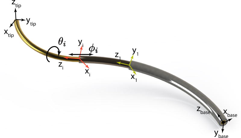
Concentric tube robots (CTR; Fig.1) alleviate these limitations by actively controlling the pose (i.e. position and orientation) of the robot’s distal end (tip) [1], [2]. Moreover, certain concentric tube robot designs enable partial control of the robot’s shape. These devices offer a means to perform elaborate tip motion, tissue interaction, and navigation of anatomical pathways. Concentric tube robots consist of precurved, superelastic tubes, which rotate and telescopically extend relative to each other. These relative motions enable shape and tip pose control. The pre-curvature, stiffness, and curved length of each tube can be computationally selected to accomplish the desired surgical tasks [3], [4], [5], which range from cardiac surgery [6], to neurosurgery [7], and prostate surgery [8].

Fig. 1.

Exemplary concentric tube robot comprising three pre-curved tubes.

CTR kinematic models predict the tip’s pose given the relative displacement of the tubes. Mechanics-based models exist that account for torsion [1], [9], friction [10], and known external forces [11], [12]. Although exteroceptive sensing via EM trackers or proprioceptive sensing via Fiber-Bragg-Gratings may also be available [13], the importance of accurate kinematics is paramount for planning and control.

Inverse kinematics provide an estimation of the relative tube motion that would yield a desired tip pose (feedforward control). Sensor measurements are then used within this scheme to reduce the estimation error further (closed loop control). Closed loop control, however, also relies on kinematics: closed-loop schemes use the robot’s inverse Jacobian to map tip-error minimizing directions onto respective tube motion. Besides control, motion planners also require a kinematic model [14], [15]. Moreover, kinematics may drive the robot ”blindly” between low-frequency measurements. Finally, accurate kinematics, combined with an appropriate recursive estimation algorithm, may provide graceful degradation in case of sensor failure.

What current approaches do not fully account for is complex nonlinear interactions between tubes. For example, existing friction models have seen limited experimental evaluation on multi-tube robots. Further, even though NiTi, the common material of concentric tubes, is well characterised, measurements of Young’s modulus and Poisson ratio for a particular tube will contain inaccuracies. Similarly, the precurvature, stiffness, and length estimations for each tube will contain errors. All these lead to misestimation of tip pose and robot shape, even when the most advanced kinematics models are used. Adaptive kinematics-model estimation is, thus, desirable. Ongoing research on online adaptation of the truncated Fourier series defining the kinematics model of [1] in [16], and neural-network-based kinematics trained through observation in [17] are preliminary approaches that address the above issues. However, both [16], [17] will overfit locally, tuning the parameters of a global model based on local information. Local regression methods can remedy the problem of overfitting by adapting only where necessary, preserving global model accuracy.

Here, we present a machine learning approach for adaptively modeling concentric tube robots kinematics based on Locally Weighted Projection Regression (LWPR) [18], yielding an accurate, non-parametric representation of the robot’s kinematics. Incoming pose measurements refine the local models at runtime, in situ, to accommodate complex non-linear phenomena. Local adaptation improves model accuracy while preserving global goodness-of-fit. Our approach is evaluated experimentally using a three-tube robot and a tip-mounted EM tracker. High accuracy across the robot’s configuration space is achieved, outperforming existing models.

II. KINEMATICS

A kinematic model is a map between two spaces: the configuration space and the task space. The configuration space for an n-tube CTR is the set of relative tube rotations α_i1 = θ_i − θ₁ and translations d_i1 = ϕ_i − ϕ₁, i ∈ {2,…,n}; both relative rotations and translations are computed with respect to the first tube. Hence, for an n-tube robot, a point in the configuration space is defined as: x = [α_i1,d_i1,…,α_n1,d_n1]^T ∈ ℝ²ⁿ⁻². The task space comprises all feasible end-effector (tip) poses. A pose is represented as a homogeneous transformation y ∈ SE(3) between a coordinate frame attached at the robot’s tip and a static reference frame attached at the robot’s base. Finally, the robot’s base can move as a rigid body in space. Hence, the full kinematic representation is defined as follows:

$$\mathbf{y}={\mathbf{H}}_{\text{base}}f(\mathbf{x})$$ (1)

where H_base ∈ SE(3) is the homogeneous transformation that accounts for the motion of the robot’s base, and f (x) : ℝ²ⁿ⁻² ↦ SE(3) is the robot’s non-linear kinematics.

In this paper, we use non-parametric regression, specifically Locally Weighted Projection Regression [18], to approximate the kinematic map f (x). This section describes the application of this technique to kinematic modeling.

A. Locally Weighted Projection Regression

Regression is used to approximate relations between variables from an input space X to an output space Y; e.g., the kinematic model f : ℝ²ⁿ⁻² ↦ SE(3). The spaces X and Y are known as the domain and range of the target function f (x). Kernel-based regression, specifically, will predict the tip’s pose f (x), for any configuration x ∈ ℝ²ⁿ⁻², using training data; i.e., tuples of the form (x_train,y_train) such that y_train = f (x_train), x_train ∈ X. Configurations close to x provide information for the robot’s tip pose f (x). Like a distance metric, a kernel quantifies proximity in the configuration space by assigning a scalar value k (weight) to any pair of robot configurations. For regression, training data for which k(x, x_j) > ε > 0 all contribute to the function estimation at x; these data correspond to robot configurations sufficiently close to the query point.

Locally Weighted Projection Regression approximates nonlinear functions using a collection of linear models. To this end, the function’s input space is partitioned into local neighborhoods. At each neighborhood, the target function is approximated by a hyperplane. To partition the space into such neighborhoods, we utilize Gaussian kernels. The mean (center) and covariance (width) define a Gaussian kernel uniquely. The Gaussian kernel assigns a weight to any point in the domain, defined as follows:

$$w(\mathbf{x})=\mathit{\text{exp}}(-\frac{1}{2}{(\mathbf{x}-\mathbf{c})}^T\mathbf{D}(\mathbf{x}-\mathbf{c}))$$ (2)

where c ∈ ℝ²ⁿ⁻² is the center of the Gaussian kernel and D⁻¹ ∈ ℝ^{(2n−2)×(2n−2)} is the covariance; equivalent to the kernel’s width. The points around the center with w > ε > 0 define the kernel’s receptive field.

Ideally, the union of all receptive fields covers the domain of the target function. In practice, this is not guaranteed, as it depends on the distribution of the training data. For each receptive field, LWPR fits training data with a linear model through Partial Least Squares (PLS; [19]). Partial Least Squares combines linear regression with dimensionality reduction. For this reason, LWPR’s accuracy is preserved for high-dimensional problems.

B. Learning

Learning the kinematic model entails partitioning the robot’s configuration space with kernels and fitting local models to each kernel’s receptive field. To this end, the center and width of each receptive field should be specified. For each neighborhood in the robot’s configuration space, the coefficients of the hyperplane that fits the training data locally are also required. All these parameters are updated by minimizing the following cost function:

$$C=\frac{{\sum }_{i=1}^M{w}_i{({\mathbf{y}}_i-{\mathbf{ŷ}}_{i,-i})}^2}{{\sum }_{i=1}^M{w}_i}+\frac{\gamma }{N}\sum _{i,j=1}^N{D}_{ij}^2$$ (3)

where (x_i, y_i) are M training examples, and ŷ_i,−i is the estimation of the target function with the i-th data point excluded from the training set [20]. In the above equation, N is the number of activated Receptive Fields. The first term in (3) is the leave-one-out-cross-validation error of the model [21]. The second term penalizes infinitely small receptive fields to avoid model overfitting. The parameters of each RF are updated by applying Stochastic Gradient Descent on cost C:

$$\mathit{\theta }≔\mathit{\theta }-\eta {\nabla }_{\mathit{\theta }}C(\mathit{\theta })$$ (4)

where θ summarizes all the training parameters of LWPR (center and width of each receptive field, local hyperplane parameters), and η is the step of the stochastic gradient descent (also known as the learning rate). The difference between stochastic and standard gradient descent lies in the computation of the cost gradient: in gradient descent, all data samples are used to compute the expected value of the gradient; whereas, stochastic gradient descent calculates the cost gradient locally at the neighborhood of the incoming training data sample. Therefore, the standard gradient descent yields a batch optimization method, whereas stochastic gradient descent affords incremental parameter updates. The update rules for the model parameters have been omitted due to space limitations; readers are referred to [18].

C. Model Prediction

Given the set of all local models, LWPR combines individual, local predictions into a final estimation of the tip’s pose. For a configuration x_q, LWPR detects all models, relevant to that estimation; namely, all models k ∈ {0,…,K} for which x_q ∈ RF_k, where RF_k denotes the receptive field of the k-th model. The kernel associated with each of the K models assigns a weight to each local prediction of the tip’s pose. The final estimation ŷ, i.e. the predicted end-effector pose, is the weighted sum of all activated model-predictions:

$$\mathbf{ŷ}={\left(\sum _{k=1}^K{w}_k\right)}^{-1}\sum _{k=1}^K{w}_k{\mathbf{ŷ}}_k$$ (5)

where w_k denotes the weight, as indicated by each kernel (see Equation (2)), and ŷ_k the local prediction of the respective model.

D. Adaptation

Using Stochastic Gradient Descent, LWPR continuously incorporates new information. LWPR’s parameters are updated as follows: when a new set of joint variables and tip pose (x_i, y_i) is provided, the algorithm first detects the activated models by checking which of the respective kernels yield weights w_k above a predefined threshold ε. Next, the activated models update the local parameters using (4). When none of the models produces a sufficiently large weight, LWPR creates a new Receptive Field, centered on this particular training sample. Given a second sample within the newly created receptive field, PLS computes the local hyperplane. This procedure is repeated as more data become available. In this way, LWPR adapts at runtime, effectively incorporating new information into the initial model. This feature is exploited to refine the kinematic model in real-time, given an initial approximation of the kinematics.

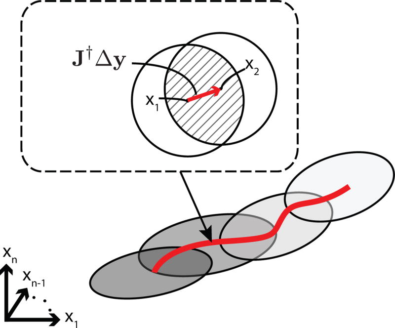
Adapting the kinematics at one point in the configuration space improves model estimation at nearby configurations, as well. While at configuration x₁, LWPR adapts all active models in the neighborhood of x₁ (see Fig. 2). The union of the receptive fields of all activated models defines a region in configuration space around x₁. Note that the same models are responsible for model prediction at x₁. Given a small displacement Δy in the task space, the robot’s configuration becomes x₂ = x₁ + J^†Δy, where J^† stands for the pseudoinverse of the robot’s Jacobian matrix J. Similarly, a new region is defined at x₂, based on the models activated by x₂. For a small Δx = x₂ − x₁ the two successive regions of activation overlap. The activated models within the overlapping region, have been already updated once when the robot was at x₁. Hence, the prediction at x₂ is improved, even before adapting again at x₂.

Fig. 2.

Model-estimation improvement due to overlapping adaptation regions.

The above concept is depicted in Fig. 2, where the gray ellipses represent activated regions as the robot moves along a trajectory in configuration space (marked as a red line). Zooming in, the activation region at x₁ (left circle) partially overlaps with activation region at x₂. The overlapping region (shaded area) is responsible for the rapid improvement of model accuracy during online adaptation. The magnitude of Δx directly influences the size of the overlapping regions, and depends on the desired displacement Δy in the workspace, as well as the magnitude of 1/det(J^T J). From that follows that close to singular configurations, where det(J^T J) → 0, the robot needs to move very slowly to maintain the overlap of successive regions of activation.

III. GENERATING A NOMINAL KINEMATIC MODEL

LWPR can be trained on a synthetic dataset to yield an initial kinematic model. The mechanics-based parametric model of [1], [12] is used here to generate a training data set. Initially, an n-dimensional grid is created, spanning the robot’s configuration space. The grid consists of equispaced points, ensuring in this way uniform sampling of the configuration space. For each configuration x, the parametric model is applied, yielding a pose y for the robot’s end-effector. The resulting {x, y} pairs are used to train the initial LWPR model.

The generated data are split into two datasets: the training and test datasets. The training dataset consists of 85% of the original data and is used to identify LWPR’s internal parameters. The remaining data (test dataset) are used to estimate the model’s generalization capability. Generating data is not essential to apply LWPR; i.e., the model can be trained online while controlling the robot. However, an initial model, even a crude one, will exhibit high accuracy much faster.

Two parameters may influence LWPR’s learning performance: the width of a newly created receptive field (D_init) and the learning rate η in (4). Initial width was chosen based on the density of the grid. Specifically, initial width was set to three times larger than the distance between successive training configurations. Model accuracy is not very sensitive to this parameter since it is refined online by the algorithm. The learning rate η is, in turn, adjusted using the Incremental Delta Bar Delta (IDBD) algorithm [22].

Relative tube rotations require some special handling. Rotational joint variables are constrained in the closed interval [−π, π] with the limit points −π, π identified. Identification declares two points equivalent. The endpoints of the line segment (corresponding to the limit points of the closed interval) are “glued” together, forming a closed loop. During distance computation, the loop can be traversed in both directions. In this way, points that are in the neighborhood of the two endpoints get closer. The distance metric should reflect this property of the target function’s domain.

To alleviate this issue, we replicate data from the bounds and extend the training dataset to [−π − ε, π + ε], ε > 0. Specifically, data that correspond to [π − ε, π] will be replicated in the range of [−π − ε, −π]; whereas, data from [−π,−π + ε] will be copied at [π, π + ε]. Modifying the dataset in this way has the same result as changing the metric, but it does not require modification of the algorithm’s implementation.

IV. EXPERIMENTS

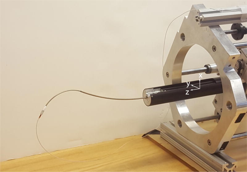
In this paper, we used the CTR shown in Fig. 3 that consists of three NiTi tubes. Tubes 1 and 2 have one constant curvature section and are equally stiff. Moreover, curved sections of both tubes have the same radius of curvature. The second tube is merely allowed to rotate relatively to the first; conversely, relative tube translation is fixed at zero (d₂₁ = 0). Based on the above, tubes 1 and 2 form a balanced pair; i.e., the combination of the two tubes at α₂₁ = π yields a straight robot body. The third tube comprises two sections: one straight and one with nonzero constant curvature. Table I summarizes all robot parameters:

Fig. 3.

Robot comprised of three tubes with tip-mounted EM sensor.

TABLE I.

Robot Parameters

	Tube 1	Tube 2	Tube 3
	Section 1	Section 1	Section 1	Section 2
Length (mm)	150	150	150	87
Curvature (m−1)	3.7736	3.7736	0	14.29
Relative Stiffness	1	1	0.2857	0.2857

The configuration space of this robot consists of all x = [α₂₁,α₃₁,d₃₁]^T, where α₂₁, α₃₁ ∈ [−π, π] and d₃₁ ∈ [0,87]. The task space consists of end-effector position and orientation. In this experiment, we controlled just the direction of z_tip (tangent vector at robot’s tip). For this reason, the representation for the orientation is merely the 3-dimensional coordinates of this unit vector. Due to the unit-vector constraint, only two of the three coordinates of z_tip are independent. Therefore, pose y belongs to a five-dimensional manifold (ℝ³ × 𝕊²) embedded in ℝ⁶. LWPR approximates the map f : ℝ³ ↦ ℝ⁶. Next, the result corresponding to z_tip is normalized to a unit vector, projecting the LWPR estimation from ℝ⁶ onto the manifold. The robot can also translate and rotate as a whole along z_base, which adds two more degrees of freedom for control. Since this is merely a rigid body transformation, LWPR does not consider these two degrees of freedom during training.

For training, we generated a 80 × 80 × 80 grid covering the robot’s configuration space uniformly. For each configuration, we computed the corresponding end-effector position, as described in Section III. Then an LWPR model was trained on the generated data. Table II provides the absolute and normalized Root Mean Square Error (RMSE) of the model predictions computed on the test dataset for all task space dimensions. For evaluating orientation accuracy, we used the relative angle between the predicted and measured tangent vectors at the robot’s tip. Next, the trained kinematics model was tested on the robot. The experimental setup consists of the three-tube robot mounted on a drive system, a haptic device (Phantom Omni) for teleoperation, and a Trackstar EM-tracker by NDI. Control software is implemented in C++ and is executed on a Intel(R) Core(TM) i7-4800MQ CPU @ 2.70GHz with 8Gb of RAM. Communication between the computer and the motors of the drive system is accomplished using a Controller Area Network (CAN) adapter with 1Mbps maximum bit-rate. The CAN adapter provides both position and velocity control of the individual motors. In all experiments, the control law is as follows:

$$\mathbf{u}={\mathbf{J}}^{†}{\mathbf{K}}_P\odot ({\mathbf{y}}_{\text{des}}-{\mathbf{y}}_{\text{current}})$$ (6)

$${\mathbf{J}}^{†}={({\mathbf{J}}^T\mathbf{J}+\epsilon \mathbf{I})}^{-1}{\mathbf{J}}^T,\epsilon >0$$ (7)

where y_des, y_current ∈ ℝ⁶ represent the goal and current end-effector pose respectively, K_P ∈ ℝ⁶ is a vector of gains, J^† is the damped least-square pseudo-inverse of Jacobian J ∈ ℝ^6×5, and ⊙ is the Schur product of two vectors (element-wise multiplication). Damped least squares inverse provides robustness to kinematic singularities [23]. J is computed numerically by successive perturbation of each joint coordinate. For Jacobian computation, the full configuration is considered; including the rigid body transformation of the base. The configuration space velocity u ∈ ℝ⁵ is applied to the motors via the CAN card.

TABLE II.

Model Validation

	x	y	z	orientation
RMSE	0.97mm	0.87mm	0.41mm	1.89 deg
nRMSE [100%]	0.68	0.58	0.52	1.05

To test model accuracy, we performed trajectory-following experiments, in which we provided the robot with time-stamped end-effector target poses. The robot used the learned kinematic model to estimate the current pose of the end-effector. We used two types of trajectories: a circular one on the x − y plane, and a random one that we recorded by teleoperating the robot.

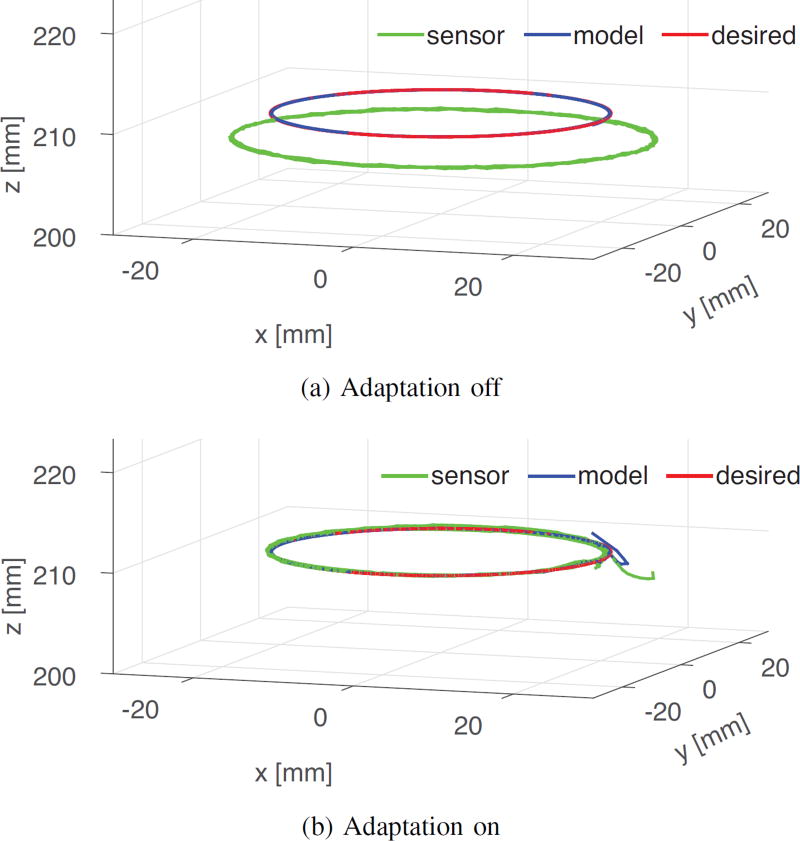
Figure 4a compares the desired, model-predicted and actual robot tip positions when moving on the commanded circle. Since model adaptation is off, there is a consistent error throughout the experiment. When adaptation is turned on, the result is shown in Fig. 4b. It is observed that the model-predicted path, and thus the sensed path, rapidly converge to the desired path.

Fig. 4.

Circular trajectory with and without online adaptation.

The speed of convergence is clearly shown in Fig. 5, which depicts model error as a function of time. The position error is less than 1mm for most of the experiment duration. Likewise, the orientation error drops to about one degree.

Fig. 5.

Difference between sensor measurements and kinematic model prediction for the circular trajectory.

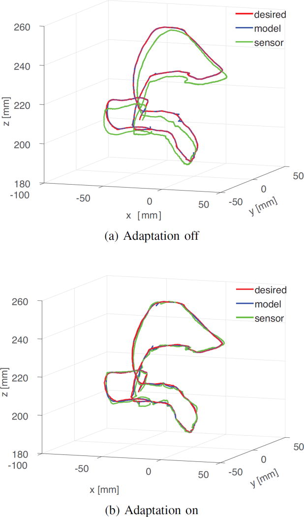
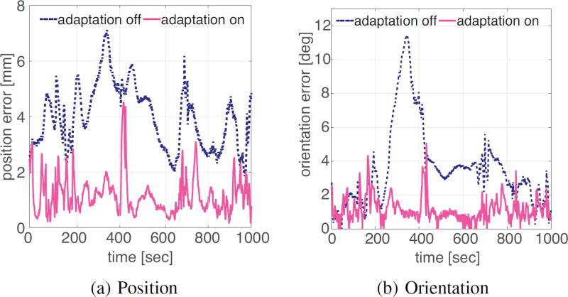
For a more general trajectory, the robot was moved under teleoperation, while recording tip pose. The resulting path is more convoluted, providing a stronger test for online adaptation. We used the recorded trajectory to perform a second set of experiments. Initially, adaptation is switched off. As previously, the initial model estimate deviates from sensor measurements. Figure 6a shows the desired trajectory juxtaposed with the model predictions and the sensor measurements. Next, we switched adaptation back on and repeated the experiment. As shown in Fig. 6b the model predictions, and consequently the actual robot trajectory, match the desired path accurately. Figure 7 shows the error of the kinematic model for the two experiments; online mode adaptation improves the prediction accuracy significantly. Table III summarizes the tracking error for both position and orientation for all experiments.

Fig. 6.

Teleoperation generated trajectory with and without online model adaptation

Fig. 7.

Difference between sensor measurements and kinematic model prediction for a trajectory generated by teleoperation.

TABLE III.

Experimental Results

trajectory	adaptation	x[mm]	y[mm]	z[mm]	θ[deg]
circle	off	3.34	3.03	2.66	2.96
circle	on	0.28	0.33	0.13	1.09
teleop	off	2.01	1.67	2.785	3.39
teleop	on	0.63	0.65	0.38	1.11

V. CONCLUSIONS

We presented a novel approximate kinematic model for Concentric Tube Robots, based on Locally Weighted Projection Regression, that approximates complex relations with multiple locally linear models. The main strength of our approach is efficient model adaptation due to incremental learning of local model parameters. The model is updated based on sensor information while it preserves goodness-of-fit across the rest of the configuration space. All the above yield an accurate kinematic representation that can account for unmodeled phenomena. Using non-parametric regression eliminates the need to define model order or parameters of any sort; all internal parameters are learned autonomously during training.

A kinematic model for a three-tube CTR was learned and evaluated on experimental data. Adaptation improved accuracy significantly on both a predefined regular shaped (circular) trajectory, as well as on a trajectory generated by teleoperation. This last experiment was performed to ensure that the algorithm performs well for random non-smooth trajectories generated such as may be generated by a surgeon during a procedure. In both experiments, adaptation substantially reduced model error.

References

- 1.Dupont PE, Lock J, Itkowitz B, Butler E. Design and control of concentric tube robots. IEEE Trans. Robotics. 2010;26(2):209–225. doi: 10.1109/TRO.2009.2035740. [DOI] [PMC free article] [PubMed] [Google Scholar]
- 2.Webster RJ, Romano JM, Cowan NJ. Mechanics of precurved-tube continuum robots. IEEE Trans. Robotics. 2009;25(1):67–78. [Google Scholar]
- 3.Bergeles C, Gosline A, Vasilyev NV, Codd P, del Nido PJ, Dupont PE. Concentric tube robot design and optimization based on task and anatomical constraints. IEEE Trans. Robotics. 2015;31(1):67–84. doi: 10.1109/TRO.2014.2378431. [DOI] [PMC free article] [PubMed] [Google Scholar]
- 4.Baykal C, Torres LG, Alterovitz R. Optimizing design parameters for sets of concentric tube robots using sampling-based motion planning; IEEE Int. Conf. Robotics and Automation; 2015. pp. 4381–4387. [DOI] [PMC free article] [PubMed] [Google Scholar]
- 5.Burgner J, Gilber HB, Webster RJ., III On the computational design of concentric tube robots: incorporating volume-based objectives; IEEE Int. Conf. Robotics and Automation; 2013. pp. 1185–1190. [Google Scholar]
- 6.Gosline AH, Vasilyev NV, Butler EJ, Folk C, Cohen A, Chen R, Lang N, Del Nido PJ, Dupont PE. Percutaneous intracardiac beating-heart surgery using metal MEMS tissue approximation tools. The International Journal of Robotics Research. 2012;31(9):1081–1093. doi: 10.1177/0278364912443718. [DOI] [PMC free article] [PubMed] [Google Scholar]
- 7.Burgner J, Rucker DC, Gilbert HB, Swaney PJ, Russell PT, Weaver KD, Webster RJ., III A telerobotic system for transnasal surgery. IEEE/ASME Trans. Mechatronics. 2014;19(3):996–1006. doi: 10.1109/TMECH.2013.2265804. [DOI] [PMC free article] [PubMed] [Google Scholar]
- 8.Hendrick RJ, Richard J, Mitchell Christopher R, Herrell S Duke, Webster Hand-held transendoscopic robotic manipulators: A transurethral laser prostate surgery case study. The International Journal of Robotics Research. 2015;34(13):1559–1572. doi: 10.1177/0278364915585397. [DOI] [PMC free article] [PubMed] [Google Scholar]
- 9.Rucker DC, Webster RJ, Chirikjian GS, Cowan NJ. Equilibrium conformations of concentric-tube continuum robots. The International Journal of Robotics Research. 2010;29(10):1263–1280. doi: 10.1177/0278364910367543. [DOI] [PMC free article] [PubMed] [Google Scholar]
- 10.Lock J, Dupont PE. Friction modeling in concentric tube robots; IEEE Int. Conf. Robotics and Automation; 2011. pp. 1139–1146. [DOI] [PMC free article] [PubMed] [Google Scholar]
- 11.Lock J, Laing G, Mahvash M, Dupont PE. Quasistatic modeling of concentric tube robots with external loads; IEEE/RSJ Int. Conf. Intelligent Robots and Systems; 2010. pp. 2325–2332. [DOI] [PMC free article] [PubMed] [Google Scholar]
- 12.Rucker DC, Jones BA, Webster RJ., III A geometrically exact model for externally-loaded concentric-tube continuum robots. IEEE Trans. Robotics. 2010;26(5):769–780. doi: 10.1109/TRO.2010.2062570. [DOI] [PMC free article] [PubMed] [Google Scholar]
- 13.Ryu SC, Dupont PE. FBG-based shape sensing tubes for continuum robots; IEEE Int. Conf. Robotics and Automation; 2014. pp. 3531–3537. [Google Scholar]
- 14.Bergeles C, Dupont PE. Planning stable paths for concentric tube robots; IEEE/RSJ Int. Conf. Intelligent Robots and Systems; 2013. pp. 3077–3082. [Google Scholar]
- 15.Torres LG, Kuntz A, Gilbert HB, Swaney PJ, Hendrick RJ, Webster RJ, Alterovitz R. A motion planning approach to automatic obstacle avoidance during concentric tube robot teleoperation; IEEE Int. Conf. Robotics and Automation; 2015. pp. 2361–2367. [DOI] [PMC free article] [PubMed] [Google Scholar]
- 16.Kim C, Ryu SC, Dupont PE. Real-time adaptive kinematic model estimation of concentric tube robots; IEEE/RSJ Int. Conf. Intelligent Robots and Systems; 2015. pp. 3214–3219. [DOI] [PMC free article] [PubMed] [Google Scholar]
- 17.Bergeles C, Lin F, Yang G. Concentric tube robot kinematics using neural networks; Hamlyn Symposium on Medical Robotics; 2015. pp. 1–2. [Google Scholar]
- 18.Vijayakumar S, D’Souza A, Schaal S. LWPR: A scalable method for incremental online learning in high dimensions. 2005 doi: 10.1162/089976605774320557. [DOI] [PubMed] [Google Scholar]
- 19.Wold H. Partial least squares. Encyclopedia of statistical sciences. 1985 [Google Scholar]
- 20.Schaal S, Atkeson CG. Constructive incremental learning from only local information. Neural computation. 1998;10(8):2047–2084. doi: 10.1162/089976698300016963. [DOI] [PubMed] [Google Scholar]
- 21.Schaal S, Atkeson CG, Vijayakumar S. Scalable techniques from nonparametric statistics for real time robot learning. Applied Intelligence. 2002;17(1):49–60. [Google Scholar]
- 22.Sutton RS. Adapting bias by gradient descent: An incremental version of delta-bar-delta. AAAI. 1992:171–176. [Google Scholar]
- 23.Siciliano B. Kinematic control of redundant robot manipulators: A tutorial. Journal of intelligent and robotic systems. 1990;3(3):201–212. [Google Scholar]