Do More of Those in Misery Suffer from Poverty, Unemployment or Mental Illness?

SUMMARY

Studies of deprivation usually ignore mental illness. This paper uses household panel data from the USA, Australia, Britain and Germany to broaden the analysis. We ask first how many of those in the lowest levels of life-satisfaction suffer from unemployment, poverty, physical ill health, and mental illness. The largest proportion suffers from mental illness. Multiple regression shows that mental illness is not highly correlated with poverty or unemployment, and that it contributes more to explaining the presence of misery than is explained by either poverty or unemployment. This holds both with and without fixed effects.

I. INTRODUCTION

Increasingly, policy-makers are considering the life-satisfaction of the population as a possible policy goal (O’Donnell et al. 2014). This makes it more important than ever to have a comprehensive account of what determines life-satisfaction. In the current debate most of the factors considered are ‘external’ to the individual – ‘situational’ factors like income, employment, family status, community safety, and religious participation (Layard et al. 2012). The chief ‘internal’ variable that is considered is general health; but this in practice relates mainly to physical health. Mental health is strikingly absent from most empirical analyses of life-satisfaction, and consequently from much of the policy debate. This may help to explain why only 5% of health expenditure in rich countries goes on average to mental health (Layard and Clark 2014).

The purpose of this paper is to remedy the omission of mental health from the analysis. The data are household panel data from the USA, Australia, Britain, and Germany. In them, a typical life-satisfaction question is “How satisfied are you with your life, all things considered?”, with possible responses on a numerical scale running from “completely dissatisfied” to “completely satisfied” – what Kahneman calls a measure of evaluated wellbeing (Kahneman 2011).

In our analysis we focus on the lowest levels of life-satisfaction (roughly the bottom 10%) which we call ‘misery’. Directly comparable results on life-satisfaction treated as a continuous variable are given in the Supplementary Information. Those results are extremely similar to the results on misery, andin themselves represent a significant contribution to the literature on life-satisfaction.

There are many reasons why the relationship between mental health and life-satisfaction has been so widely overlooked in the wellbeing debate. One is the fact that mental illness is a subjective state and so is life-satisfaction. But our data have a key advantage: they include the most “objective” measures available of mental illness – that the person has been diagnosed with depression/anxiety by a health professional, or that the person is in treatment. In addition, because individuals are observed over several years, we can examine how mental illness and misery co-vary within the same lifetime.

Even so, some people might argue that mental illness and misery are the same thing. In this paper we show that, to the contrary, the correlation between misery and mental health (between 0.1 and 0.4) is not high enough to suggest they are measures of the same construct. We find that there are many causes of misery but mental illness is one important cause, even holding constant all other causes.

So treating mental illness directly is one way to reduce misery (Roth and Fonagy 2005). But how large a part should the treatment of mental illness play in a strategy to reduce misery? This depends on how big a problem mental health is compared with other problems: how much of the misery in a society is associated with mental illness, as opposed to issues like poverty, unemployment or physical ill-health? That is what this paper is about.

In what follows we begin with the simplest possible, descriptive question: What are the characteristics of the most miserable sections of the community? As we show, many more of those in the lowest levels of life-satisfaction suffer from mental illness than from unemployment, poverty or physical illness. This is true in all four countries. We then move to multivariate analysis where we find that the presence or absence of mental illness explains more of the variance of misery than is explained by either poverty, unemployment or physical illness. This is true in cross-sectional analysis, but also using fixed effects or including the lagged dependent variable.

II. DATA AND METHODS

Our analysis uses five household surveys, all of which provide information on both life-satisfaction and on mental health. Three of these surveys have the key advantage of including “objective” data on whether the person has been diagnosed with depression/anxiety, with two of them also including data on whether the person is in treatment for a mental health problem. These three surveys are: for the USA, the Behavioral Risk Factor Surveillance System (BRFSS) and the Panel Study of Income Dynamics (PSID); and for Australia, the Household, Income and Labour Dynamics in Australia (HILDA) Survey.

Of these, the BRFSS is purely cross-sectional, giving data on different people for 2006–2013. But the two other studies have data on the same individual’s diagnostic condition for two different years. This enables us to examine the effect of changes in mental health on changes in life-satisfaction, thus mitigating the influence of unobserved individual characteristics.

However, to obtain multiple repeated observations on the same individual, we have to use data on self-reported symptomatology of mental illness provided by three household panel surveys: for Australia, HILDA annually 2001–2010; for Britain, the British Household Panel Survey (BHPS) annually 1996–2008; and for Germany, the German Socio-Economic Panel (GSOEP) biannually 2002–2008.

All the five surveys provide information on income, employment, family status, education and physical health. Thus we can isolate the impact of mental and physical health on misery, holding constant other potential sources of misery. All the data are from representative samples of people aged 25 and over, and all variables are based on questionnaires set out in full in the Supplementary Information (SI).

II.1. Mental illness

Mental illness is measured either by “objective” data (as above) or by self-reported mental health symptomatology (in Australia from the Short Form 36 Health Survey; in the UK from the General Health Questionnaire 12; and in Germany from the Short Form 12 Health Survey). We exclude “happy” items from the Short Form Health Survey and the General Health Questionnaire.

II.2. Misery

We define misery as being in the bottom levels of life-satisfaction. The exact proportion of the population in misery differs between countries because life-satisfaction is measured in discrete integers. Misery in Australia is the bottom 7.5% of life-satisfaction (0–5 on a scale from 0 to 10); in the US (BRFSS) the bottom 5.6% (1–2 on a scale from 1 to 4); in the US (PSID) the bottom 6% (1–2 on a scale from 1 to 5); in Britain the bottom 9.9% (1–3 on a scale from 1 to 7) and in Germany, the bottom 8.7% (0–4 on a scale from 0 to 10).

II.3. Other variables

Physical health is defined in the U.S. by the number of health conditions diagnosed by a health professional; in Australia and Germany by self-reported symptomatology; and in Britain by the self-reported number of conditions. Household income is equivalised, with household income per adult equivalent equal to the family income divided by (1 + 0.7(other adults) + 0.5 children). All regression equations also control linearly for age, age², living with a partner, education and gender – known to be significant predictors of life-satisfaction.

Not all questions are asked in all years and when they are included they are not always answered.¹ In each analysis we include only observations for which there are replies to all questions, sample sizes being reported in each table. Means and standard deviations of all variables are shown with the Correlation Matrices in the SI.

III. RESULTS

III.1. Descriptive statistics

We begin in Figure 1 with descriptive statistics, to see what percentage of the people in misery have different specific characteristics.

Figure 1.

Percentage of Those in Misery Having the Characteristics Shown. Australia. United States (BRFSS).

Notes: Misery in Australia is the bottom 7.5% of life-satisfaction, and in the United States (BRFSS) the bottom 5.6%. In Australia, the sample size is 16,896 (and 8,855 for the question on treatment). In US, the sample size is 268,300 (and 217,225 for the question on treatment). In Australia, 40 % of the least satisfied segment of the population are poor when poverty is defined as the bottom 20% and in the United States, 47%. The analysis for the USA was first published in Layard and Clark (2014).

In Australia only 20% of the least satisfied segment of the population are poor. The proportion who are unemployed is even smaller. By contrast 48% of those in misery have ever been diagnosed with depression or anxiety disorders, and 31% are currently in treatment. The position in the USA is broadly similar: many more of the least satisfied segment of the population have mental health problems than are poor or unemployed.

What accounts for these differences? Two forces are at work. The first is how likely people with each condition are to be miserable, relative to the likelihood in the general population. Without implying causality, we can call this the “relative impact” of the factor. The second is the overall “prevalence” of the condition in the total population. Thus, if M_i is the number in misery who have condition i, M is the total number of people in misery, T_i is the total number of people with condition i in the population, and T is the total population, then the numbers in Figure 1 are given by.

$$\frac{\text{Mi}}{\mathrm{M}}\equiv \frac{\text{Mi}/\mathrm{T}}{\mathrm{M}/\mathrm{T}}\equiv \frac{\mathrm{T}}{\mathrm{T}}\equiv \text{Relative impact × Prevalence}$$

Table 1 uses this breakdown to account (arithmetically) for the share of the dissatisfied who have each characteristic.

Table 1.

Decomposition of Sources of Misery

	% of those in misery having each characteristic		≡	Relative impact of each characteristic on misery		X	% Prevalence of each characteristic
	(1)		(2)			(3)
Australia
Poor (bottom 10%)	20	(0.4)		2.0	(0.1)		10	(0.1)
Unemployed	7	(0.3)		2.9	(0.1)		2.5	(0.1)
Ever diagnosed with depression/anxiety	48	(1.4)		2.6	(0.1)		18	(0.3)
Currently in treatment for a mental health condition	31	(1.7)		3.4	(0.2)		9	(0.3)
Physical health problems (bottom 10%)	22	(0.5)		2.2	(0.05)		10	(0.1)
United States (BRFSS)
Poor (bottom 10%)	27	(0.1)		2.7	(0.1)		10	(0.0)
Unemployed	13	(0.1)		3.2	(0.1)		4	(0.0)
Ever diagnosed with depression/anxiety	61	(0.4)		2.7	(0.1)		22	(0.1)
Currently in treatment for a mental health condition	40	(0.4)		3.0	(0.1)		13	(0.1)
Physical health problems (bottom 10%)	14	(0.1)		1.4	(0.0)		10	(0.0)

Notes. Standard errors in parentheses. Misery in Australia is the bottom 7.5% of life-satisfaction and in the United States (BRFSS) the bottom 5.6%. In Australia, the sample size is 16,896 (and 8,855 for the question on treatment). In US, the sample size is 268,300 (and 217,225 for the question on treatment).

The high share of those who are mentally ill, compared with the share who are poor, is due to a mixture of the greater prevalence of mental illness and its greater relative impact. There is no danger that we have overstated the importance of mental illness since the prevalence of a mental health diagnosis in these surveys is rather below the prevalence in specific household surveys of psychiatric morbidity (McManus et al. 2009; Kessler et al. 2005; Wittchen and Jacobi 2005). The table also suggests that physical health problems (as measured) have a somewhat lower relative impact than mental health problems.

Description is a proper way to start. But an obvious question is whether much of the mental illness is not itself due to poverty and unemployment, in which case the proper policy priority might be to focus on reducing poverty and unemployment rather than directly attacking mental illness. To answer this question requires multivariate analysis.

III.2. Cross-sectional regressions

We choose to use linear multiple regression, with misery as the dependent variable treated as a 0/1 dummy variable. We also use logit analysis which gives almost identical results (shown in the SI). But linear multiple regression using standardised variables has a major advantage: the resulting partial correlation coefficients (or β-statistics) shown in Table 2 reflect the “power” of each variable to explain the presence or absence of misery, holding all other variables in the equation constant. They therefore reflect the impact of the variable times its standard deviation, which in the case of a dichotomous variable is $\sqrt{\left(T_i/T\right)\left(1-T_i/T\right)}$ where Ti/T is its prevalence.

Table 2.

Predictors of Misery: Cross-section Analysis (partial correlation coefficients)

	Australia						United States (BRFSS)
Income (log)	−0.08	(17)	−0.06	(7)	−0.05	(5)	−0.14	(27)	−0.12	(14)	−0.13	(19)
Unemployed	0.07	(12)	0.06	(5)	0.05	(3)	0.07	(41)	0.06	(18)	0.07	(14)
Ever diagnosed with depression/anxiety			0.14	(14)					0.17	(44)
Currently in treatment for mental health condition					0.12	(9)					0.16	(39)
Physical health problems	0.17	(34)	0.16	(14)	0.16	(10)	0.09	(35)	0.05	(14)	0.09	(22)
N Observations	81,285		16,896		8,855		1,961,708		268,300		217,225
R2	0.061		0.090		0.097		0.055		0.084		0.082

Notes. Robust t-statistics in parentheses. Controls for age, age², living with partner, education, and gender.

To increase the explanatory power of income and physical health, we now treat them as continuous variables. Table 2 shows the results. Each column represents one equation. For each country the first equation omits mental health, and therefore shows the standardised ‘effect’ of income and unemployment in a way that includes their effects via mental health. As the t-statistics show, the effects are highly significant. But, when we introduce mental health, the effects barely change. This is because of the strikingly low correlation between mental health and income or unemployment. Moreover, once mental health is introduced, it exerts a bigger influence on misery than either income or unemployment.

How about the comparison of mental with physical health? In the table the mental health variables (which are binary) have similar explanatory power to the continuous physical health variables. But it is difficult to draw clear conclusions due to possible problems of measurement. To help with this problem, the BRFSS provided a separate measure of mental health that is exactly analogous to a measure of physical health: each respondent was asked “For how many days during the past 30 days was your mental health not good?”, and an identical question for physical health. The replies to the mental health question had a much stronger predictive power than those on physical health (β = 0.31 and 0.11 respectively), even though the most miserable people reported almost the same number of days with bad mental and physical health (15 and 13 days respectively). The overall conclusion must be that mental and physical illness have similar power to explain misery, and in both cases greater power than variations in income or employment.

The analysis so far is purely cross-sectional. It barely begins to approach any attempt at causality – for example, the cross-sectional correlations are partly the product of permanent genetic or personality differences affecting both the correlated variables. We can come closer to causality by looking at the same individual at multiple points in time, and examining how changes in different variables within the same person are interconnected.

III.3. Time-series descriptive statistics

We begin with the two surveys which give two years of repeated data on the diagnostic state of the same individual. These are HILDA and the U.S. PSID. (In the PSID the percentage of diagnosed mental illness is only 7%, much smaller than is normal in household surveys of psychiatric morbidity (McManus et al. 2009; Kessler et al. 2005; Wittchen and Jacobi 2005) which is why we have not used it earlier.)

We can start again with simple descriptive statistics. Table 3 examines those people who entered misery within a given period, and asks what else changed in their lives over the same period. In Australia 14% of these people had acquired a diagnosis of depression or anxiety disorder, while only 7% had become poor, 6% had become unemployed, and 8% had become physically ill. In the United States the role of recent poverty in explaining newly-acquired misery was greater than that of mental illness, partly due to the narrow definition of mental illness and partly due to the huge flows in and out of poverty.

Table 3.

Decomposition of Sources of Newly-Acquired Misery

	% of those entering misery who have each characteristic		≡	Relative impact of each characteristic upon entering misery		X	% of population who have each characteristic
Australia (2007 to 2009)
Became poor (bottom 10%)	7.3	(1.3)		1.9	(1.1)		3.7	(0.2)
Became unemployed	5.9	(1.2)		3.5	(1.5)		1.7	(0.1)
Became diagnosed with depression/anxiety	13.5	(2.1)		2.4	(0.7)		5.6	(0.3)
Became physically ill (bottom 10%)	8.4	(1.7)		2.1	(1.0)		3.9	(0.2)
USA (PSID) (2009 to 2011)
Became poor (bottom 10%)	19.1	(1.5)		3.2	(0.5)		5.9	(0.1)
Became unemployed	11.1	(1.2)		2.3	(0.7)		4.9	(0.1)
Became diagnosed with emotional, nervous or psychiatric problems	13.3	(1.3)		3.9	(0.5)		3.4	(0.1)
Became physically ill (bottom 10%)	8.6	(1.1)		2.7	(0.4)		3.2	(0.1)

Notes. Standard errors in parentheses. Misery in Australia is the bottom 7.5% of life-satisfaction and in the USA (PSID) the bottom 6%. In Australia, the sample size is 16,896. In US, the sample size is 27,095.

III.4. Time-series regressions

However to get nearer to causality we have to look simultaneously at the impact of all variables and to include movements out of misery as well as into it. This is done in Table 4, which is the dynamic equivalent of Table 2. For each country we start with equations including a fixed effect for each individual. This removes the effect of all permanent differences between individuals. When this is done, the coefficients on all variables are substantially reduced, as the comparison for Australia shows. For example, in the case of mental illness we have removed the effect of all permanent differences between individuals in their mental health. But diagnosed mental illness remains a more important explanation of the fluctuation in misery over the life-course than are either income or unemployment. The same is true in the U.S. using the PSID.

Table 4.

Predictors of Misery: Dynamic Analysis (partial correlation coefficients)

	Australia				United States (PSID)
Income (log)	−0.01	(0.3)	−0.03	(4.0)	−0.04	(2.7)	−0.06	(6.0)
Unemployed	0.02	(1.3)	0.05	(3.8)	0.02	(2.3)	0.05	(7.0)
Ever diagnosed with depression/anxiety*	0.04	(1.8)	0.10	(11.5)	0.09	(5.7)	0.08	(10.4)
Physical health problems	0.08	(4.0)	0.11	(12.2)	0.04	(2.6)	0.03	(4.4)
Misery in previous year			0.33	(20.2)			0.24	(29.9)
N Observations	16,896		15,767		27,095		12,450
R2	0.010		0.186		0.006		0.116
Individual fixed effect	YES		NO		YES		NO

Notes. Robust t-statistics in parentheses. Controls for age, age², living with partner, education, and gender.

^*In the U.S. “emotional, nervous or psychiatric problems”.

An alternative way to investigate the dynamics of misery is by replacing the fixed effect by the lagged dependent variable. This takes out less of the fixed effect but also allows for other lagged effects of the observed and unobserved variables. This procedure is used in the remaining columns of Table 4 and again shows mental illness as a more important explanatory factor than income or unemployment.

III.5. Analyses using self-reported symptomatology

The major limitation of the preceding analysis is that we only have data on diagnosed illness for two years. By contrast, if we use self-reported symptoms as the basis for identifying mental illness, we have many more years data from the Australian, British and German household panel surveys (up to 9, 12 and 6 years respectively). Figure 2 shows for these countries the share of misery accounted for by people in the bottom 10% of self-reported mental health. Even if we measure this variable six years earlier, it accounts for more of those in misery than are accounted for by being in poverty or unemployment today.

Figure 2.

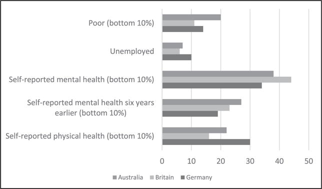
Percentage of Those in Misery Having the Characteristics Shown.

Notes. Those in misery comprise the bottom 7.5% of life-satisfaction in Australia, the bottom 9.9% in Britain, and the bottom 8.7% in Germany.

But again, to attempt to move towards causality, we need to run multiple regressions. Table 5 shows the results of such analysis including fixed effects and treating mental health as a continuous variable. This shows that when we include measures of current symptoms, the estimated effect of mental health is larger than in our previous tables. But this could partly reflect time-varying fluctuations in reporting style. When, to obviate this problem, we replace current by lagged mental health, the explanatory power of mental health is less – but most frequently greater than that of current income or employment.

Table 5.

Predictors of Misery: Using Symptomatology and Fixed Effects (partial correlation coefficients)

	Australia				Britain				Germany
Income (log)	−0.02	(2.8)	−0.01	(1.7)	−0.02	(3.6)	−0.02	(3.5)	−0.03	(5.0)	−0.02	(2.2)
Unemployed	0.03	(5.1)	0.03	(4.1)	0.02	(5.4)	0.03	(6.6)	0.03	(3.6)	0.04	(5.1)
Self-reported mental health problems	0.15	(24.9)			0.33	(60.9)			0.23	(24.8)
Self-reported mental health problems in previous year			0.02	(3.3)			0.08	(15.0)			0.06	(7.2)
Physical health problems	0.03	(3.7)	0.06	(7.9)	0.03	(5.6)	0.06	(10.2)	0.04	(5.6)
Physical health problems in previous year											0.03	(3.5)
N Observations	81,285		67,003		126,987		113,522		53,407		53,699
N Individuals	15,375		12,652		20,758		18,672		22,673		20,041
R2	0.029		0.007		0.096		0.009		0.049		0.007
Individual fixed effect	YES		YES		YES		YES		YES		YES

Notes. Robust t-statistics in parentheses. Controls for age, age², living with a partner.

IV. DISCUSSION

We have shown that, to understand the sources of misery, one should look not only at traditional variables like income, employment and physical health but also at mental health. Though we do not claim anywhere to have a fully causal analysis, our results suggest that mental illness is an important form of deprivation, which receives far too little attention, even within the health sector.²

Indeed our findings confirm earlier work comparing the effects of physical and mental illness. Here Graham et al. and Dolan and Metcalfe have regressed life-satisfaction on reported mental and physical pain using the EQ5D, and found that mental pain had a bigger effect than physical pain (Graham et al. 2011; Dolan and Metcalfe 2012). Those studies were cross-sectional (as was another (Mukuria and Brazier 2013)), but in a further study Dolan et al. repeated the analysis using two separate observations per person, with similar results (Dolan et al. 2012). The authors hypothesised that mental pain is more difficult to adapt to – it occupies more of a person’s mental space. Like their work, our results strongly suggest that health policy should give greater weight to mental health and that the weights used in calculating QALYs should be reconsidered (Dolan and Kahneman 2008).

However when it comes to policy-making, two more key questions are the efficacy of treatment and the cost. To compare these, the policy-maker will want to evaluate their effects on life-satisfaction, which is a preferred policy measure to ‘misery’ (O’Donnell et al. 2014). So how does treatment increase life-satisfaction, and how does cost reduce it?

We can illustrate this by considering the case for better access to cognitive behavioural therapy for people with depression or anxiety disorders. We shall use coefficients from the life-satisfaction regressions shown in the SI. On the benefit side these show that, holding constant the fixed effect, acquiring a diagnosis in the USA reduces life-satisfaction by 0.3 standard deviations (.07/.26). So losing a diagnosis raises life-satisfaction by an equal amount, and from field trials we know that therapy leads at least 1 in 3 to recover who would not otherwise have done so (Roth and Fonagy 2005). So treatment yields an average gain of 0.1 standard deviations of life-satisfaction per person treated, lasting for at least a year.

This has to be compared with the cost. The therapy costs some 5% of average annual income per person, which is about 0.05 standard deviations of annual equivalised log income in the USA. This reduces annual life-satisfaction by 0.0015 standard deviations (0.05 × 0.03). This compares with the benefit of 0.1 standard deviations: the benefit is some 70 times the cost.

In practice the cost would of course be spread across more people than those who benefit from the treatment, but this spreading of the cost would only serve to reduce its total impact. For Australia the ratio of benefit to cost is about 10 times. These calculations are extremely rough but simply illustrate how this approach could provide policy-makers with a quite new perspective on orders of magnitude.

The analysis of the paper is of course subject to a host of caveats. The analysis is not fully causal, though it becomes more so through the inclusion of fixed effects or the lagged dependent variable. Moreover, question-ordering can introduce spurious correlation between variables (Schwarz and Strack 1999). For example, in the BHPS mental health questions precede the question on life-satisfaction and the former may influence the latter. But the BRFSS, PSID and GSOEP ask about life-satisfaction before mental health, and HILDA asks the question on separate occasions. Moreover in fixed effects analysis the bias resulting from question-ordering largely disappears provided the question-ordering does not change.

We conclude that time-varying mental health really has an important independent influence on life-satisfaction. And so surely does the non-varying component of mental health, though this is less easily studied. There are policy implications. For too long the debate on deprivation has focussed mainly on poverty, jobs, education and physical sickness. It needs broadening to include the inner person (Layard 2014).

References

- Boyce CJ, Wood AM, Powdthavee N. Is personality fixed? Personality changes as much as “variable” economic factors and more strongly predicts changes to life satisfaction. Social Indicators Research. 2013;111(1):287–305. [Google Scholar]
- Diener E, Seligman M. Very happy people. Psychological Science. 2002;13(1):81–84. doi: 10.1111/1467-9280.00415. [DOI] [PubMed] [Google Scholar]
- Dolan P, Kahneman D. Interpretations of utility and their implications for the valuation of health. Economic Journal. 2008;118(525):215–234. [Google Scholar]
- Dolan P, Metcalfe R. Valuing health: a brief report on subjective well-being versus preferences. Medical Decision Making. 2012;32(4):578–82. doi: 10.1177/0272989X11435173. [DOI] [PubMed] [Google Scholar]
- Dolan P, Lee H, Peasgood T. Losing sight of the wood for the trees: Some issues in describing and valuing health, and another possible approach. PharmacoEconomics. 2012;30(11):1035–49. doi: 10.2165/11593040-000000000-00000. [DOI] [PubMed] [Google Scholar]
- Graham C, Higuera L, Lora E. Which health conditions cause the most unhappiness? Health Economics. 2011;20:1431–1447. doi: 10.1002/hec.1682. [DOI] [PubMed] [Google Scholar]
- Headey B, Kelley J, Wearing A. Dimensions of mental health: Life satisfaction, positive affect, anxiety and depression. Social Indicators Research. 1993;29:63–82. [Google Scholar]
- Kahneman D. Thinking, fast and slow. London: Allen Lane; 2011. [Google Scholar]
- Kessler RC, Chiu WT, Demler O, Merikangas KR, Walters EE. Prevalence, severity, and comorbidity of 12-month DSM-IV disorders in the National Comorbidity Survey Replication. Archives of General Psychiatry. 2005;62(6):617–627. doi: 10.1001/archpsyc.62.6.617. [DOI] [PMC free article] [PubMed] [Google Scholar]
- Layard R. Mental Health: the new frontier for labour economics. In: McDaid D, Cooper CL, editors. Wellbeing: A complete reference guide Volume 5 The economics of wellbeing. Oxford: Wiley-Blackwell; 2014. [Google Scholar]
- Layard R, Clark DM. Thrive: the power of evidence-based psychological therapies. London: Penguin; 2014. [Google Scholar]
- Layard R, Clark AE, Senik C. The causes of happiness and misery. In: Helliwell JF, Layard R, Sachs J, editors. World Happiness Report. New York: The Earth Institute, Columbia University; 2012. pp. 58–89. [Google Scholar]
- McManus S, Meltzer H, Brugha T, Bebbington P, Jenkins R, editors. Adult psychiatric morbidity in England, 2007: results of a household survey. Leeds: The Health & Social Care Information Centre, Social Care Statistics; 2009. [Google Scholar]
- Mukuria C, Brazier J. Valuing the EQ-5D and the SF-6D health states using subjective well-being: A secondary analysis of patient data. Social Science & Medicine. 2013;77:97–105. doi: 10.1016/j.socscimed.2012.11.012. [DOI] [PubMed] [Google Scholar]
- O’Donnell G, Deaton A, Durand M, Halpern D, Layard R. Wellbeing and policy. London: Legatum Institute; 2014. [Google Scholar]
- Roth A, Fonagy P, editors. What works for whom? A critical review of psychotherapy research. Second. New York: Guilford Press; 2005. [Google Scholar]
- Schwarz N, Strack F. Reports of Subjective Well-Being: Judgmental Processes and Their Methodological Implications. In: Kahneman D, Diener E, Schwarz N, editors. Well-Being: The Foundations of Hedonic Psychology. New York: Russell Sage Foundation; 1999. [Google Scholar]
- Vazquez C, Rahona JJ, Gomez D, Caballero FF, Hervas G. A National Representative Study of the Relative Impact of Physical and Psychological Problems on Life Satisfaction. Journal of Happiness Studies. 2015;16(1):135–148. [Google Scholar]
- Wittchen HU, Jacobi F. Size and burden of mental disorders in Europe: a critical review and appraisal of 27 studies. European Neuropsychopharmacology. 2005;15:357–376. doi: 10.1016/j.euroneuro.2005.04.012. [DOI] [PubMed] [Google Scholar]
Associated Data
This section collects any data citations, data availability statements, or supplementary materials included in this article.