Potential and limitations of inferring ecosystem photosynthetic capacity from leaf functional traits

Abstract

The aim of this study was to systematically analyze the potential and limitations of using plant functional trait observations from global databases versus in situ data to improve our understanding of vegetation impacts on ecosystem functional properties (EFPs). Using ecosystem photosynthetic capacity as an example, we first provide an objective approach to derive robust EFP estimates from gross primary productivity (GPP) obtained from eddy covariance flux measurements. Second, we investigate the impact of synchronizing EFPs and plant functional traits in time and space to evaluate their relationships, and the extent to which we can benefit from global plant trait databases to explain the variability of ecosystem photosynthetic capacity. Finally, we identify a set of plant functional traits controlling ecosystem photosynthetic capacity at selected sites. Suitable estimates of the ecosystem photosynthetic capacity can be derived from light response curve of GPP responding to radiation (photosynthetically active radiation or absorbed photosynthetically active radiation). Although the effect of climate is minimized in these calculations, the estimates indicate substantial interannual variation of the photosynthetic capacity, even after removing site‐years with confounding factors like disturbance such as fire events. The relationships between foliar nitrogen concentration and ecosystem photosynthetic capacity are tighter when both of the measurements are synchronized in space and time. When using multiple plant traits simultaneously as predictors for ecosystem photosynthetic capacity variation, the combination of leaf carbon to nitrogen ratio with leaf phosphorus content explains the variance of ecosystem photosynthetic capacity best (adjusted R ² = 0.55). Overall, this study provides an objective approach to identify links between leaf level traits and canopy level processes and highlights the relevance of the dynamic nature of ecosystems. Synchronizing measurements of eddy covariance fluxes and plant traits in time and space is shown to be highly relevant to better understand the importance of intra‐ and interspecific trait variation on ecosystem functioning.

1. Introduction

Accurate predictions of land–atmosphere feedbacks under climate change require an in‐depth understanding of how climatic and other environmental controls on ecosystem functioning are mediated by vegetation characteristics, diversity, and structure (Bonan, 2008). Eddy covariance (EC) measurements of carbon dioxide (CO₂), water, and energy fluxes are widely employed to monitor ecosystem processes and functions (Baldocchi et al., 2001). The increased number of EC flux sites contributing to the FLUXNET network allows for monitoring ecosystem processes and responses to environmental conditions for different ecosystems and time scales (Baldocchi, 2008). In many applications, both in terrestrial biosphere models and in experimental analyses, the characteristics and structure of the vegetation are given by plant functional types (PFTs), which represent a grouping of functionally similar plant types (Lavorel, Mcintyre, Landsberg, & Forbes, 1997). However, plant traits and model parameters derived from EC data can be highly variable within PFTs and species (Alton, 2011; Groenendijk et al., 2011; Kattge et al., 2011; Reichstein, Bahn, Mahecha, Kattge, & Baldocchi, 2014). Vegetation characteristics and the variation therein are assumed to be determined by the abundance and traits of the respective plant species (Garnier et al., 2004; Lavorel & Garnier, 2002). Therefore, both modeling (Pappas, Fatichi, & Burlando, 2016; Van Bodegom et al., 2012; Verheijen, Aerts, Bonisch, Kattge, & Van Bodegom, 2015) and observational efforts (Meng et al., 2015) increasingly aim to account for the variation of traits within and between PFTs, in order to better understand the relationship between vegetation characteristics and ecosystem functioning. Most efforts so far have focused on specific regions (e.g., Ollinger et al., 2008) and have not systematically analyzed the importance of spatiotemporal variation in traits and ecosystem functional variables for their relationship. Plant traits contribute to different ecosystem processes where our knowledge is often limited. Furthermore, efforts have mostly focused on leaf nitrogen as a functional trait (in relation to ecosystem productivity, e.g., Kattge, Knorr, Raddatz, & Wirth, 2009), whereas other plant traits could also be suitable candidates. Foliar phosphorus, for example, improves the model prediction of carbon fluxes as reported by Mercado et al. (2011), Goll et al. (2012), and Yang, Thornton, Ricciuto, and Post (2014).

The short‐term (half‐hourly to daily) variability of carbon fluxes measured with the EC technique is controlled by meteorological, environmental conditions (Richardson, Hollinger, Aber, Ollinger, & Braswell, 2007), and endogenous plant controls (De Dios et al., 2012). In contrast, biotic responses (e.g., temporal variability in plant abundance and traits) seem to be more important than environmental variation for long‐term (e.g., annual) variation of fluxes (Richardson et al., 2007; Stoy et al., 2009). Evaluating the relationship between plant traits and eddy covariance fluxes is not straight forward because the former is usually measured only a couple of times per year (mostly during the growing season), whereas the latter is measured continuously at half‐hourly intervals. It is possible to derive so‐called ecosystem functional properties (EFP) from EC measurements, a concept recently introduced to characterize the long‐term patterns underlying carbon, water, and energy fluxes (Musavi et al., 2015; Reichstein et al., 2014).

The EFPs are ecosystem properties related to physical and ecohydrological parameters relevant for land surface–atmosphere interactions (Reichstein et al., 2014) and are assumed to be affected by vegetation characteristics. Analogous to leaf level ecophysiological characteristics, such as carboxylation capacity (Vc_max), EFPs are less variable in time than the fluxes themselves, which makes them a suitable quantity to be linked to plant functional traits (Musavi et al., 2015; Reichstein et al., 2014). Therefore, EFPs can be used to characterize long‐term variation in key process characteristics, such as ecosystem photosynthetic capacity and respiration rates under standardized environmental conditions, or they can represent the sensitivity of processes to temperature and light availability (for a more detailed collection; see Table 1, Musavi et al., 2015). Deriving EFP estimates from EC fluxes is not trivial, because they should represent intrinsic ecophysiological properties of the ecosystem; effects of short‐term meteorological conditions on functional responses should be factored out.

Table 1.

Definitions of ecosystem photosynthetic capacity estimated using light response curve

Ecosystem photosynthetic capacity	Radiation	Definition
GPPsat	PAR	GPP at light saturation using PAR as driving radiation and 2110 μmol m−2 s−1 as saturating light
GPPsat.structure	APAR	GPP at light saturation using APAR as driving radiation and 2000 μmol m−2 s−1 as saturating light
A max	PAR	Light saturated GPP—parameter of Equation (1) with PAR as driving radiation
A max.sructure	APAR	Light saturated GPP—parameter of Equation (1) but with APAR as driving radiation
GPPcum	PAR	Integral of the light curve GPP up to the saturation point 2110 μmol m−2 s−1 of PAR
GPPcum.structure	APAR	Integral of the light curve GPP up to the saturation point 2000 μmol m−2 s−1 of PAR

In the column “Radiation,” the independent variable used in Equation (1) is reported.

Another constraint for testing the links between plant traits and EFPs is that so far, measurements of plant functional traits have not yet been carried out systematically at FLUXNET sites. Consequently, a number of studies linking plant traits and EFPs using a wide range of ecosystems are few (e.g., Kergoat, Lafont, Arneth, Le Dantec, & Saugier, 2008). Although plant trait data from FLUXNET sites are currently limited, the global database of plant traits—TRY (Kattge et al., 2011)—facilitates the identification of many different traits for most of the plant species present at FLUXNET sites, which could potentially help testing such relationships. However, the use of trait values derived from such broadscale databases may suffer from inaccuracies, when trait values for a particular site deviate from those reported in databases, which may hamper deducing the patterns of plant traits influences on EFPs. Hence, it is important to test the potentials and limitations of using plant functional traits derived from a global database (e.g., TRY) versus in situ measurements obtained from the sites to infer the impact of plant traits on ecosystem processes derived from EC flux data. We still do not know how temporal and spatial variations in both EFPs and plant functional traits are linked. Likewise, the uncertainties of the relationship between EFPs to plant functional traits related to the temporal dynamics of both ecosystem functioning and traits have not been evaluated before. This is the first time to our knowledge that the relationship between an EFP (here ecosystem photosynthetic capacity) derived from EC CO₂ fluxes and plant traits and the associated uncertainties have been systematically investigated for spatiotemporal variation and the relevance of synchronized observations. Using ecosystem photosynthetic capacity as an example for an EFP derived from selected FLUXNET sites, the goals of this study were as follows:

1. Providing an objective approach to characterize ecosystem photosynthetic capacity from different estimates of gross primary productivity (GPP) derived from EC measurements.

2. Assessing how relaxing the time‐space synchronization of ecosystem photosynthetic capacity estimates and plant functional trait measurements introduces uncertainty to their relationships (with a particular focus on leaf nitrogen content per leaf mass).

3. Identifying (a set of) plant traits that control the spatial variability (i.e., across sites) of ecosystem photosynthetic capacity.

2. Materials and Methods

The overall methodological approach consisted of comparing different ways to estimate ecosystem photosynthetic capacity at each FLUXNET site. Ecosystem photosynthetic capacity is an EFP related to the photosynthetic processes at ecosystem scale. It is computable from estimates of GPP from EC, incoming photosynthetically active radiation (PAR) and the fraction of absorbed photosynthetically active radiation (FAPAR) retrieved from remote sensing. Given the attempt to characterize properties related to long‐term variation of ecosystem function that are not affected by short‐term meteorological variability, the ecosystem photosynthetic capacity estimates with the least interannual variation (IAV) were assumed as the most appropriate to characterize the EFP. These estimates of ecosystem photosynthetic capacity were correlated with leaf nitrogen content per leaf mass (N) measured in situ or derived from the TRY database to identify the relevance of time and space synchronizing measurements of EC data and plant traits. Finally, ecosystem photosynthetic capacity was correlated with a suite of other photosynthesis‐related plant traits to identify those that control its spatial (i.e., across site) variability.

2.1. Eddy covariance flux measurements

The analysis used data from the FLUXNET La Thuile database (Baldocchi, 2008), referred hereafter as “La Thuile.” Very dry sites and forest site‐years with disturbances (i.e., forest thinning, harvesting, and planting) were removed opting for optimal conditions to avoid confounding factors. For the remaining dataset, 20 sites responded to a request for providing leaf traits sampled in 2011/2012 (for some sites, trait measurements from previous years were used) and the flux data from the year of sampling. Depending on the site, different years of flux data were available in the La Thuile database in addition to the fluxes from the sampling year 2011/2012.

To characterize ecosystem photosynthetic capacity, we used half‐hourly values of GPP (μmol CO₂ m⁻² s⁻¹) and the corresponding PAR (μmol m⁻² s⁻¹). The GPP values were computed using the commonly used algorithm for flux partitioning, which is based on the extrapolation of nighttime net ecosystem exchange measurements using an ecosystem respiration model based on air temperature (Reichstein et al., 2005). As PAR was not always available at the selected sites, we derived PAR by multiplying global incoming shortwave radiation (Rg, Wm⁻²) by 2.11 (Britton & Dodd, 1976).

Only GPP data derived from measured net ecosystem exchange were used for the analysis and gap‐filled values were omitted. In addition, only daytime GPP data were used (Rg > 10 Wm⁻²). For each site‐year, we estimated the number of days with more than 80% gaps in half‐hourly net ecosystem exchange measurements during the period from April to September. Site‐years with more than 25% of such days were excluded.

2.2. MODIS TIP‐FAPAR and leaf area index (LAI)—vegetation structure

For the selected sites, estimates of FAPAR and LAI (see Pinty et al., 2011a,b) derived at 1 km spatial resolution by the JRC‐TIP (Pinty et al., 2007) from the MODIS broadband visible and near‐infrared surface albedo products (Schaaf et al., 2002) were used to quantify the vegetation phenology and changes in the structure of the ecosystem with 16‐day temporal resolution (Musavi et al., 2015; Figure 1). We used the FAPAR time series of the pixels where the towers of FLUXNET sites were located. To fill gaps in FAPAR and LAI, we performed a distance correlation between the time series of all pixels around the central pixel for each flux site (Szekely, Rizzo, & Bakirov, 2007). We subsequently chose pixels with a correlation of r > .75 with the central pixel. Afterward, we used the data of those pixels to fill the gaps in the central pixel, prioritizing the pixels with highest correlation. In case where gaps remained after this procedure, we used a spatiotemporal gap‐filling approach for the remaining gaps (v. Buttlar, Zscheischler, & Mahecha, 2014). To derive daily time series of FAPAR, a smoothing spline approach was used to derive daily time series of FAPAR (see also Filippa et al., 2016; Migliavacca et al., 2011). FAPAR was then used to compute half‐hourly APAR (absorbed photosynthetic active radiation) values (μmol m⁻² s⁻¹). Annual maximum LAI was derived using the 90^th percentile of the satellite retrieved estimates of LAI from JRC‐TIP of the same year of sampling (Pinty et al., 2011a).

Figure 1.

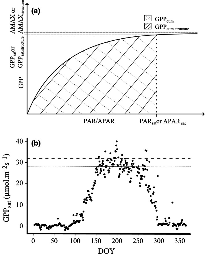
(a) Conceptual figure of the different estimates of ecosystem functional property (EFP) related to ecosystem photosynthetic capacity. Light response curves are fitted using GPP flux and PAR or APAR according to Table 1. (b) Time series of GPP _sat for 1 year. Higher values of GPP _sat occur during the growing season (usually around mid‐spring to end‐summer). For this study, we use the 90th percentile as the maximum GPP _sat of each year, which is indicated with the dashed line. For comparison the 60th percentile of GPP _sat is indicated with the dotted line

2.3. Plant functional trait collection—vegetation characteristics

Plant traits known to be relevant for photosynthesis at ecosystem scale, specifically leaf nutrient content and stoichiometry of the nutrients, were determined (Sardans & Penuelas, 2012): leaf nitrogen content per dry mass (N_mass or per 100 g leaf dry mass‐ N%), leaf nitrogen content per leaf area (N_area, g/m²), leaf phosphorus content per leaf dry mass (P_mass, mg/g) and per leaf area (P_area, g/m²), leaf carbon content per leaf dry mass (C, mg/g), leaf C/N ratio (C/N, g/g), leaf stable isotope concentration (δ¹³C), and specific leaf area, (SLA, mm/mg).

In situ leaf samples from the selected sites were collected in the period 2011–2012 (except for two sites in 2003 and in 2004). The leaf sampling protocol was based on “Protocols for Vegetation Sampling and Data Submission” of the terrestrial carbon observations panel of the global terrestrial observing system (Law et al., 2008). Samples were collected from the dominant species present in the footprint of the flux towers (defined by the site's principal investigator). Depending on accessibility, multiple individuals per species were sampled. Sampling was carried out mostly at peak growing season on fully developed and nondamaged leaves and from different levels of the canopy (top, middle, and bottom, representing fully sunlit and shaded leaves). For forest sites, the understory vegetation was not sampled.

After grinding the dried leaves, total carbon and nitrogen concentrations were determined by dry combustion with an elemental analyzer (Perkin Elmer 2400 Series II). Phosphorus concentrations were determined by digesting ground leaf material in 37% HCl: 65% HNO₃. Phosphorus was subsequently measured colorimetrically at 880 nm after a reaction with molybdenum blue. δ¹³C was determined by an elemental analyzer (NC2500, ThemoQuest Italia, Rodana, Italy) coupled online to a stable isotope ratio mass spectrometer (Deltaplus, ThermoFinnigan, Bremen, Germany). Leaf area was calculated with the ImageJ freeware (http://rsb.info.nih.gov/ij/).

Species abundance information was collected for each site, or if not available (e.g., for one tropical forest site), all species were considered equally abundant. Abundance information for each species was used to calculate the community weighted means (CWM, Garnier et al., 2004) of the different plant traits considered in the analysis: foliar N, P, and C concentration of leaves, SLA, and δ¹³C. Plant trait data were also extracted from the TRY global database (Kattge et al., 2011). Species mean values were calculated from the observed plant trait values included in TRY, which were subsequently used to compute CWM trait values at each site. TRY data used in this study based on the following references: Atkin, Westbeek, Cambridge, Lambers, & Pons, 1997; Bahn et al., 1999; Campbell et al., 2007; Cavender‐Bares, Keen, & Miles, 2006; Coomes, Heathcote, Godfrey, Shepherd, & Sack, 2008; Cornelissen, 1996; Cornelissen et al., 2003; Cornelissen, Diez, & Hunt, 1996; Cornelissen et al., 2004; Cornwell et al., 2008; Craine et al., 2009; Craine, Lee, Bond, Williams, & Johnson, 2005; Diaz et al., 2004; Freschet, Cornelissen, Van Logtestijn, & Aerts, 2010; Fyllas et al., 2009; Garnier et al., 2007; Han, Fang, Guo, & Zhang, 2005; Hickler, 1999; Kattge et al., 2011, 2009; Kazakou, Vile, Shipley, Gallet, & Garnier, 2006; Kerkhoff, Fagan, Elser, & Enquist, 2006; Kleyer et al., 2008; Laughlin, Leppert, Moore, & Sieg, 2010; Louault, Pillar, Aufrere, Garnier, & Soussana, 2005; Loveys et al., 2003; Medlyn et al., 1999; Messier, Mcgill, & Lechowicz, 2010; Meziane & Shipley, 1999; Niinemets, 2001; Ogaya & Penuelas, 2003; Onoda et al., 2011; Ordonez et al., 2010; Poorter, Niinemets, Poorter, Wright, & Villar, 2009; Poschlod, Kleyer, Jackel, Dannemann, & Tackenberg, 2003; Quested et al., 2003; Reich, Oleksyn, & Wright, 2009; Reich et al., 2008; Sack, Cowan, Jaikumar, & Holbrook, 2003; Sack, Melcher, Liu, Middleton, & Pardee, 2006; Shipley, 1995, 2002; Shipley & Vu, 2002; Vile, 2005; White, Thornton, Running, & Nemani, 2000; Willis et al., 2010; Wright et al., 2007, 2004, 2010.

2.4. Estimates of ecosystem photosynthetic capacity

To estimate the ecosystem photosynthetic capacity, we used ecosystem level light response curves, using half‐hourly GPP estimates and a variety of radiation data. The resulting six different formulations of ecosystem photosynthetic capacity estimates are reported in Table 1 and described in the following.

We fitted nonrectangular hyperbolic light response curves (Gilmanov et al., 2003):

$$\text{GPP}=\frac{1}{2\mathrm{\theta }}\left(\mathrm{\alpha }Q+A_{\max }-\sqrt{{\left(\mathrm{\alpha }Q+A_{max}\right)}^2-4\mathrm{\alpha }{A}_{max}\mathrm{\theta }Q}\right)$$ (1)

where α is the initial slope of the light response curve, θ is the curvature parameter (ranging from 0 to 1), A _max is the plateau of the light response curve, GPP is the half‐hourly GPP values, Q is the incoming radiation used to drive the model. Specifically, two different estimates of radiation were used (PAR, and APAR): In the estimation of the EFPs, APAR was used to account for seasonal and across‐site variations in canopy structure (e.g., LAI) as it stands for the amount of light that is absorbed by the leaves of the ecosystem.

The ecosystem photosynthetic capacity values were estimated using a 5‐day moving window. The parameters of the light response curves were estimated and attributed to the day at the center of the window (Figure 1a). The parameters were estimated by minimizing the model observation residual sum of square with the quasi‐Newton optimization method that allows box constraints (Byrd, Lu, Nocedal, & Zhu, 1995). To this purpose, we used the optim function implemented in R (http://CRAN.R-project.org/). For comparison, a Michaelis–Menten‐based light response curve (Hollinger et al., 2004) was used. Results were comparable with the nonrectangular hyperbolic light response curve (data not shown).

Each light response curve fitting was used to derive the A _max parameter, the value of GPP at light saturation and the integral of the light response curve at light saturation (Falge et al., 2001). For light saturation, we defined a threshold of Rg of 1,000 Wm² (corresponding to PAR of 2,110 μmol m⁻² s⁻¹) (see also Jacobs et al., 2007). This resulted in six different estimates describing ecosystem photosynthetic capacity: (1) A _max: parameter of the Equation (1); (2) A _{max.structure}: parameter of Equation (1) but with APAR as driving radiation to account for canopy structure; (3) GPP_sat: GPP at light saturation using PAR as driving radiation (4) GPP_{sat.structure}: as GPP_sat but with APAR as radiation variable; (5) GPP_cum: integral of the fitted light response until light saturation; and (6) GPP_{cum.structure}: as GPP_sat but using APAR as radiation until light saturation (Figure 1a, Table 1).

A time series of daily values of A _max, A _{max.structure}, GPP_sat, GPP_{sat.structure}, GPP_cum, and GPP_{cum.structure} was then derived for each year. In Figure 1b, GPP_sat is shown as an example. Daily parameters were retained for further analysis only if the R ² of the fit of light response curve was higher than 0.6. In this way, we first retain parameters estimated when the performance of the fitting is good, and second, we retain data only in the active growing season as the R ² of the model fit was typically higher than 0.6 only within the growing season (Fig. S1).

To extract the corresponding annual ecosystem photosynthetic capacity for each site‐year, maximum and different percentiles (90th to 60th) of the time series of the estimated parameters were computed. Finally, the coefficient of variation (CV, Everitt, 1998) of the annual ecosystem photosynthetic capacity estimates was computed for each site. For example, at each site, we computed the annual value for GPP_sat (i.e., 90th percentile of GPP_sat daily time series). The CV was subsequently computed as the standard deviation of annual GPP_sat of all years available, divided by the mean annual GPP_sat for all years available at the respective site (CV GPP_sat). The CV was used as a measure of the interannual variability (IAV) of the ecosystem photosynthetic capacity estimates. Low IAV (i.e., the lowest CV) was used as criteria to identify the most appropriate estimates to characterize the ecosystem photosynthetic capacity at each site. This was repeated for both ecosystem photosynthetic capacity estimates with and without the effect of canopy structure included (i.e., using PAR and APAR, respectively). This comparison was made using sites with at least 5 years of data. The average of annual ecosystem photosynthetic capacity of the selected estimates was used to relate to leaf functional traits.

2.5. Relationship between ecosystem photosynthetic capacity and leaf nitrogen concentration

This study evaluates the relevance of synchronizing measurements of plant functional traits and EFPs in space and time for joint analyses. We analyzed the relationship between the best estimates for ecosystem photosynthetic capacity selected as described above, and CWM of plant traits, for example, N%. N% is chosen here, as the relationship between N% and photosynthetic processes is well established (e.g., Field & Mooney, 1986; Reich, Walters, & Ellsworth, 1997) at the leaf scale and to a lesser extent at ecosystem scale (e.g., Kergoat et al., 2008; Ollinger et al., 2008). The relationship with other traits is included in the supporting information (Fig. S2). Three different combinations of synchronizing ecosystem photosynthetic capacity and N% were tested:

(1) Ecosystem photosynthetic capacity derived from the La Thuile database and species N% derived from TRY (no synchronization in space and time); (2) ecosystem photosynthetic capacity derived from the La Thuile database and the N% sampled at the FLUXNET sites (in situ, synchronization in space); (3) ecosystem photosynthetic capacity derived for the same year of trait sampling and N% in situ (synchronization in space and time).

For each combination of ecosystem photosynthetic capacity and N%, the slope and R ² of the linear regression were determined. Distance correlation was computed as well, as it accounts for nonlinear relationships (Szekely et al., 2007). In order to evaluate the predictive capacity of the selected model, a leave‐one‐out cross‐validation was performed. Modeling efficiency (EF; Loague & Green, 1991) and relative root mean square error (RRMSE) were computed to test the performances of the relationships. An analysis of covariance (ANCOVA) was conducted to statistically test the differences of regression slopes in the three relationships. In addition, to assess the significance of canopy structure in the relationship of plant traits and ecosystem photosynthetic capacity, we evaluated the information that LAI, representing the canopy structure, provides to the relation of N% and photosynthetic capacity estimated using GPP and PAR.

2.6. Identifying plant functional traits controlling ecosystem photosynthetic capacity

Because the functional relationship between plant traits, their interactions and photosynthetic capacity is not yet completely defined (Sardans & Penuelas, 2012), a purely data‐driven approach was used (Golub, 2010). To identify the main explanatory variables (plant functional traits and LAI) of ecosystem photosynthetic capacity, we used a stepwise multiple regression for variable selection based on the Akaike's information criterion (AIC; Yamashita, Yamashita, & Kamimura, 2007). Plant traits used in this context include N%, N_area, P_mass and P_area, C, δ¹³C, and SLA. We allowed the variables (traits and LAI) to be raised to the half and second power and also included the logarithm and ratios of all predictors to account for nonlinear relationships and interactions as well.

3. Results

3.1. Identifying robust estimates to characterize ecosystem photosynthetic capacity

Among the different percentiles that were used for the extraction of annual ecosystem photosynthetic capacity estimates, the 90th percentile was the one that minimized the CV (i.e., the IAV) of most estimators (Figure 2). The maximum annual values showed the highest IAVs and therefore were not considered appropriate estimates of ecosystem photosynthetic capacity. The use of the 60th percentile for the extractions showed slightly higher IAV than the 90th percentile. Other percentiles such as 85, 80, 75, and 70 were also tested and had similar results to the 60 percentile (data not shown). However, considering that we were interested in the annual maximum photosynthetic rates the 90th percentile of the different parameters was selected for further analyses.

Figure 2.

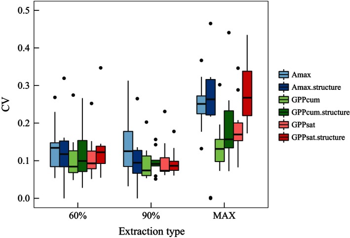
Comparison of mean and ranges of the different estimates of ecosystem photosynthetic capacity and different annual extractions. CV denotes the coefficient of variation (standard deviation/mean), which was calculated for every site. The results are based on sites with at least 5 years of available estimates (AT‐Neu, DE‐Hai, FI‐Hyy, FR‐Hes, IL‐Yat, IT‐MBo, IT‐Ren, IT‐SRo, NL‐Loo, RU‐Fyo). The lines across the box indicate the mean CV values and lower and upper boxes show the 25th and 75th percentiles. The lines on the ending of the boxes range from the maximum to minimum values. CV can be used to quantify the interannual variability of the estimates (small range and low average denote low interannual variability). For explanations of the ecosystem photosynthetic capacity estimates described in the legend, see Table 1

Among the different estimators for ecosystem photosynthetic capacity (Table 1), A _max and A _{max.structure} had the highest IAV regardless of how they were extracted annually. GPP_cum and GPP_sat had the lowest IAV, even though a detailed analysis revealed a substantial IAV for both estimators at some La Thuile sites (Figure 3). While GPP_cum is related to the whole growing season, GPP_sat is related mostly to the peak of growing season. However, GPP_cum and GPP_sat were strongly correlated (Table S1). GPP_{cum.structure} and GPP_{sat.structure}, accounting for canopy structure, showed slightly higher IAV than GPP_cum and GPP_sat. As we aimed at developing a method to derive maximum ecosystem photosynthetic capacity robust to meteorological variability, we assessed the impact of excluding from the analysis site‐years with documented extreme events, such as the heat wave of 2003 in Europe (Fig. S3). Removing the year 2003 from the European site‐years did not change the results (Fig. S4). In addition, the estimated parameters, for example, GPP_sat were not strongly linked to climate variables (Fig. S8).

Figure 3.

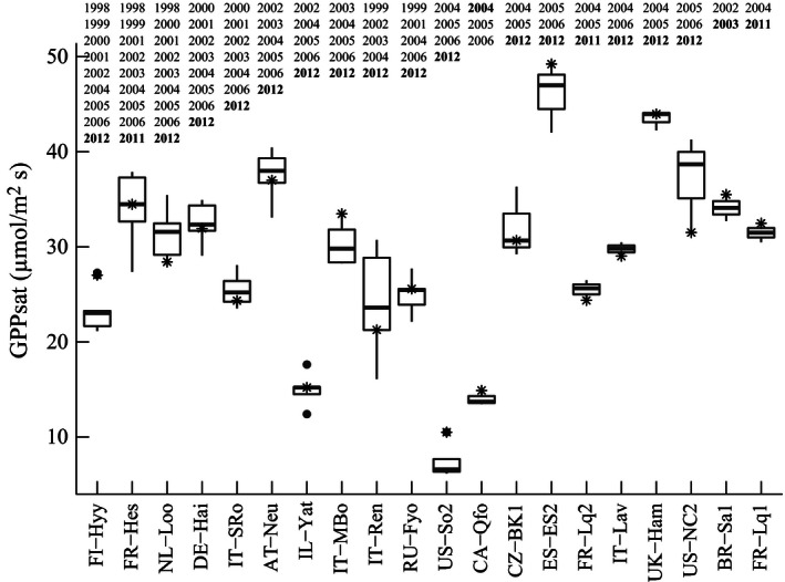
Boxplots of annual GPP _sat values derived from the La Thuile database for each FLUXNET site. The line across the boxplot shows the mean GPP _sat for each site, and the lower and upper boxes show the 25th and 75th percentiles of GPP _sat. The stars denote GPP _sat values of the respective sites in the year of in situ plant trait measurements (bold years)

We concluded that the 90th percentile of GPP_cum or GPP_sat parameters of nonrectangular hyperbolic light response curves (either with or without structural information included) was an appropriate approach to characterize ecosystem photosynthetic capacity.

3.2. Relationship between ecosystem photosynthetic capacity and plant functional traits

Using a linear relationship, the N% based on data from the TRY database explained 27% of the variance of site averaged GPP_sat (20% of GPP_{sat.structure}) (Figure 4a, Table 2). N% derived from TRY and in situ were strongly correlated (Fig. S5), and the R ² of the relationship between N% and GPP_sat, and GPP_{sat.structure} improved from 0.27 to 0.39 and from 0.20 to 0.32, respectively, when in situ N% was used (Figure 4b, Table 2). In addition, site averaged estimates of GPP_sat and GPP_{sat.structure} were replaced by GPP_sat and GPP_{sat.structure} from the years of in situ sampling R ² increased to 0.50 and 0.37, respectively (Figure 4c, Table 2). The fit is even better when a nonlinear fit was used for Figure 4a,b (distance correlation increased from 0.56 to 0.73 for GPP_sat and from 0.47 to 0.63 for GPP_{sat.structure,} See also Fig. S6). An ANCOVA test revealed that the relationship between ecosystem photosynthetic capacity and N% was significantly different between the levels of synchronization when GPP_sat (significantly different in slope and intercept, p < .01) or GPP_{sat.structure} (only significantly different intercept, p < .05) was used to characterize ecosystem photosynthetic capacity. Similar improvements of the relationship of CWM traits to GPP_sat and GPP_{sat.structure} were realized using other plant traits and synchronizing the plant traits with the ecosystem photosynthetic capacity estimates in time and space (Fig. S2). We also tested whether the improvement of this relationship was due to random effects. To do this, we randomly resampled the annual photosynthetic capacity (specifically GPP_sat and GPP_{sat.structure}) to test whether the use of corresponding years statistically improves the relationship or not. The results confirmed that the best fit was obtained when the N% and the photosynthetic capacity estimate match in time and space (Table S2).

Figure 4.

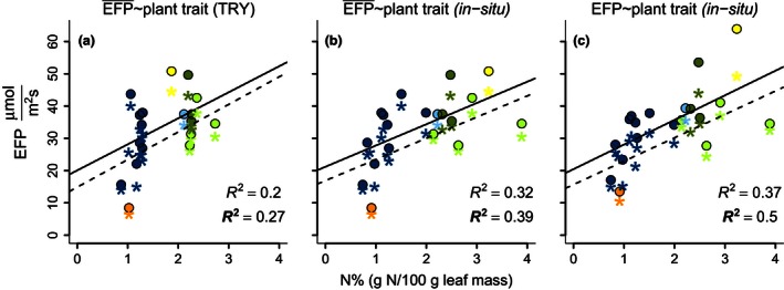
Relationship between a) GPP _sat and GPP _{sat.structure} extracted from La Thuile and N% from TRY, b) GPP _sat and GPP _{sat.structure} from La Thuile and N% in situ, c) GPP _sat and GPP _{sat.structure} derived from the same year of the trait sampling and N% in situ. Y‐axes are ecosystem photosynthetic capacity as an example of an EFP, and x‐axes are community weighted N%. The Macro accent on the EFP indicates that the GPP _sat and GPP _{sat.structure} are the multiyear averages for each site. Bold R ² and star symbols are for the relationships with ecosystem photosynthetic capacity estimates using PAR (GPP _sat). Nonbold R ² and round points are for the relationship with ecosystem photosynthetic capacity estimates using APAR (GPP _{sat.structure}). The colors dark blue, light blue, dark green, light green, orange and yellow represent evergreen needle leaf forest, evergreen broad leaf forest, deciduous broad leaf forest, grassland, closed shrub‐land, and cropland as the plant functional types of the sites, respectively

Table 2.

Statistics of the relationships shown in Figure 4

Ecosystem photosynthetic capacity	Model	Distance correlation	R 2	adj. R 2	Intercept ± SE	Slope ± SE	p	RRMSE	EF	df
GPPsat	N%	0.73	0.50	0.47	15.67 ± 3.51	7.25 ± 1.71	.0005	26.2	0.31	1 + 18
$\overline{GP{P}_{\mathrm{sat}}}$	N%	0.67	0.39	0.36	16.89 ± 3.95	6.57 ± 1.93	.003	29.09	0.18	1 + 18
$\overline{GP{P}_{\mathrm{sat}}}$	N%TRY	0.56	0.27	0.23	14.88 ± 5.74	8.55 ± 3.28	.018	30.65	0.09	1 + 18
${\mathrm{GPP}}_{\mathrm{sat}.\mathrm{structure}}$	N%	0.63	0.37	0.34	20.45 ± 5	7.62 ± 2.39	.005	30	0.10	1 + 17
$\overline{GP{P}_{\mathrm{sat}.\mathrm{structure}}}$	N%	0.58	0.32	0.28	21.18 ± 4.87	6.59 ± 2.33	.01	25.5	−0.15	1 + 17
$\overline{GP{P}_{\mathrm{sat}.\mathrm{structure}}}$	N%TRY	0.47	0.20	0.15	20.08 ± 7.01	8.07 ± 3.94	.06	26.1	−0.20	1 + 17

Ecosystem photosynthetic capacity estimates with macron accent are averaged over several years at each site and those without macron accent are from the year of leaf sampling. RRMSE and EF are estimated in a cross‐validation with leave‐one‐out mode and represents, relative root mean square error, and model efficiency, respectively. The number of FLUXNET sites that are used with GPP^sat are 20, but 19 of the sites have GPP_{sat.structure} available.

As species abundance information at the FLUXNET sites can be a relevant source of uncertainty, we also calculated site‐level species‐averaged N% without accounting for differences in abundance. The results of the R ² decreased but only by about 0.05 (Fig. S7).

Part of the unexplained variance may be due to the fact that we used leaf level N%, while not accounting for differences in LAI. Indeed, although N% and LAI are highly correlated, the combination of N% and LAI led to a better explanation of the variability of GPP_sat, (adjusted R ² = 0.56, R ² = 0.64) than N% (R ² = 0.50) or LAI (R ² = 0.28) alone (Table 3—for 19 sites with available LAI).

Table 3.

Relationships between N%, LAI, and GPP_sat tested

Variable	Model	Distance correlation	R 2	adj. R 2	Intercept ± SE	Slope ± SE	p	df	AIC
LAI	N%	0.70	0.48	0.45	0.34 ± 0.38	0.71 ± 0.18	.001	1 + 17	44
GPPsat	LAI	0.57	0.28	0.24	20.10 ± 4.03	5.43 ± 2.09	.01	1 + 17	138
GPPsat	N%	0.73	0.50	0.47	15.25 ± 3.79	7.41 ± 1.81	.0008	1 + 17	132
GPPsat	LAI + N%	0.71	0.50	0.44	14.96 ± 3.98	N% 6.78 ± 2.58LAI 0.87 ± 2.51	.004	2 + 16	134
GPPsat	N% + LAI + LAI:N%	—	0.64	0.56	0.74 ± 6.94	N% 15.22 ± 4.22LAI 10.33 ± 4.55N%:LAI −4.71 ± 1.98	.001	3 + 15	129

The GPP_sat is derived from the year at which the sampling of leaf N% was carried out. N% here is measured from in situ samples. LAI is the 90th percentile of the bimonthly LAI values retrieved from remote sensing and corresponds to the LAI of the sampling year as well (available for 19 sites).

3.3. Essential plant traits for ecosystem photosynthesis capacity

The variable selection analysis conducted with the stepwise regression using time‐space synchronized data of ecosystem photosynthetic capacity estimates and in situ measured plant traits and LAI showed that the variability of GPP_sat and GPP_{sat.structure} between sites is best explained by leaf C/N ratio and P_area ² (considering AIC as the selection criteria). However, only C/N was a significant predictor for both of the ecosystem photosynthetic capacity estimates. The selected model explained 61% and 54% of the variance of GPP_sat and GPP_{sat.structure}, respectively (Table 4).

Table 4.

Results of the variable selection analyses conducted with a stepwise regression

Variable	Model	Distance correlation	R 2	adj. R 2	Intercept ± SE	Slope ± SE	p	df	AIC	EF
GPPsat	C/N + Parea 2	0.67	0.61	0.55	41.62 ± 3.01	C/N −0.39 ± 0.08Parea 2 23.94 ± 16.20	.0009	2 + 15	119	0.18
GPPsat.structure	C/N + Parea 2	0.65	0.54	0.48	49.02 ± 4.07	C/N −0.48 ± 0.12Parea 2 38.89 ± 22.22	.004	2 + 14	123	−0.28

The selected explanatory variables for GPPsat are C/N + P_area ². The same variables are tested for GPP_sat.structure as well. Subsets of sites are used because only 18 sites had these two traits available and GPP_sat and only 17 have the two traits and GPP_{sat.structure} measurements.

4. Discussion

4.1. Determining robust estimates of an EFP

We postulated that the IAV of ecosystem photosynthetic capacity at optimal growth conditions (e.g., at optimal light, temperature, and water availability) derived with the proposed methodology and in the absence of disturbances should be low, and we demonstrated that it is not strongly related to climate drivers (Fig. S8). Additionally, assuming that the variation of plant traits across years is relatively low, this would allow for coupling ecosystem photosynthetic capacity estimates at any year, or averaged over several years, to species traits collected at the respective site (typically sampled during peak growing season).

Based on these criteria, the use of the light response curves was suitable as it accounts for variation in radiation, which is one of the important parameters explaining variation in GPP (Van Dijk, Dolman, & Schulze, 2005). The estimation of the parameters using a moving window approach was also suitable because it accounts for variation in meteorological variables such as temperature and vapor pressure deficit. Among the parameters derived from the light response curve, A _max (or A _{max.structure}) had the largest IAV and was therefore the least suitable estimator for ecosystem photosynthetic capacity. This may have several reasons: The response of GPP to PAR/APAR does not exhibit a clear saturation and still tends to increase at high PAR/APAR and reaches A _max outside the range of PAR/APAR measurements. Therefore, small changes in the slope at high PAR/APAR may cause large deviations in A _max (Gilmanov et al., 2003). In periods of the year when the PAR/APAR is not high, or the numbers of data points at high PAR is limited, the A _max parameter is poorly constrained. In this case, the fit can be affected by random flux uncertainty that scales with the magnitude of fluxes and is not easily constrainable (Richardson et al., 2012). GPP_sat or GPP_cum showed much smaller IAV, and therefore, we suggest the use GPP_sat or GPP_cum derived with PAR or APAR (Falge et al., 2001; Lasslop et al., 2010; Ruimy, Jarvis, Baldocchi, & Saugier, 1995) as more robust estimators of ecosystem photosynthetic capacity than A _max. Our results also demonstrate that the use of higher percentiles (i.e., 90th) rather than the maximum for EFP extraction should be preferred as it was more robust to outliers.

4.2. Linking plant functional traits and EFP estimates

Ecosystem functional properties are whole‐ecosystem properties and thus depend on both ecosystem structure and function (Reichstein et al., 2014). As GPP depends on both the efficiency with which the absorbed energy is converted to chemical energy at leaf level (Monteith, 1972) and the canopy structure, GPP_sat variability ultimately depends on the variability of FAPAR (Reichstein et al., 2014). In this study, we accounted for this aspect using APAR in Equation (1) for the estimation of GPP_{sat.structure}. APAR accounts for the seasonal and canopy structural (e.g., LAI) variability of the different ecosystems (Wang & Jarvis, 1990). In extreme combinations, it is possible for an ecosystem to maintain a high LAI but low N% and vice versa (Mcmurtrie et al., 2008; Fig. S9). However, due to the smoothing and reconstruction of time series of daily FAPAR from 16‐day data (e.g., Kandasamy, Baret, Verger, Neveux, & Weiss, 2013), and the spatial mismatch between satellite pixel and the eddy covariance footprint (Cescatti et al., 2012; Jung et al., 2008; Roman et al., 2009), the EFP estimates using APAR exhibited larger uncertainties that more likely is reflected in the higher IAV compared to using PAR. The FAPAR product that we used for our estimates has a high temporal resolution (16 days) but its spatial resolution (1 km) makes it uncertain; the footprints of FLUXNET sites are often smaller than a 1 km grid cell, and sites located in heterogeneous grid cells have higher uncertainties in FAPAR as a consequence (Cescatti et al., 2012). Nevertheless, the relationships of the estimates of photosynthetic capacity to plant traits were consistent, whether PAR or APAR was used. Our results also indicate the importance of accounting for canopy structure (Baldocchi & Meyers, 1998; Reich, 2012). The LAI‐N% interaction contributes to the explanatory power of the model for predicting GPP_sat, as it shows how N% has an approximately linear relationship with GPP_sat (i.e., the GPP at light saturation without accounting for canopy structure) while the impact of LAI saturates.

A critical aspect when comparing leaf level attributes and EFPs is scaling these traits from leaf to canopy level. Based on the hypothesis that the dominant species are most adapted to their ambient environment (Vile, Shipley, & Garnier, 2006), also known as “dominance hypothesis” (Grime, 1998), we used CWM estimates of traits from dominant species at the sites. Here, we considered sites with different vegetation types and environments (e.g., climate), where differences between the locations and vegetation types are large enough to ignore intraspecific trait variability, this allows us to use averaged trait values from TRY database in this study and in likewise global scale analyses (see Albert, Grassein, Schurr, Vieilledent, & Violle, 2011).

4.3. Robustness of ecosystem photosynthetic capacity–plant trait relationship to relaxed time‐space synchrony of measurements

Here, we show that the general pattern of the relationship between ecosystem photosynthetic capacity and plant traits (slopes of the linear regression, Figure 4) is apparently independent using locally measured traits (in situ) or species mean values from the TRY database. In addition, the relationships are independent of whether all data corresponded to the same year or the ecosystem photosynthetic capacity represented the multiyear averages of ecosystem photosynthetic capacity we used (most cases, Fig. S2). However, we observed a strong degradation of the explained variance when the synchronization in time and space was relaxed. The predictive power of plant functional traits for ecosystem photosynthetic capacity substantially improved when variation of species abundance, intraspecific variability of plant traits, and interannual variability of ecosystem photosynthetic capacity were accounted for.

In part, this variability may be due to community species composition dynamics and competitive interactions that are partly triggered by disturbances or extreme environmental conditions. The study sites were not chosen to be in their late successional stage, and in the course of, for example, 10 years of flux measurements, species abundances can change and plant species can be replaced. Site history and aging of the ecosystems contributes to the variability of the plant traits (Becknell & Powers, 2014) and EFPs (e.g., Kutsch et al., 2009; Urbanski et al., 2007). This includes also the effect of fertilization on few sites, which could be one of the reasons why the in situ N% from the cropland and grasslands are very different from the mean N% from TRY. Plant traits also have a temporal variability, which can be due to plant development or changes in the environment (e.g., Mickelbart, 2010). Plant traits are responsible for the plastic response of an ecosystem to environmental changes and thus influence the interannual variability of ecosystem photosynthesis (Grassi, Vicinelli, Ponti, Cantoni, & Magnani, 2005; Ma, Baldocchi, Mambelli, & Dawson, 2010). Furthermore, it confirms that species signals of some traits, specifically leaf nutrients, are not strong enough (high trait variability) (Kazakou et al., 2014) and this contribute to the uncertainty observed when linking EFPs and trait values derived from data bases. One way to account for intraspecific trait variation is to use trait observations from TRY that were reported from similar climatic conditions to the FLUXNET sites, or to predict intraspecific trait variation (Schrodt et al., 2015). These opportunities are promising for future work, but could not be used here due to data scarcity and insufficient prediction accuracy. It remains to be better understood how the intraspecific variation of plant traits in time contributes to the response of plant communities to hydrometeorological changes and thus how the interannual and long‐term variability of ecosystem photosynthetic capacity is mediated by dynamics of the vegetation (Reichstein et al., 2014). A promising approach to monitor long‐term variation of plant traits for different FLUXNET sites worldwide is novel remote sensing information (e.g., Asner & Martin, 2015; Asner, Martin, Anderson, & Knapp, 2015). But the contribution of physiological vs. structural information in the remote sensing signals needs to be better understood (e.g., Homolova, Maenovsky, Clevers, Garcia‐Santos, & Schaeprnan, 2013; Wong & Gamon, 2015). The common protocols developed in initiatives like ICOS—integrated carbon observation system (https://www.icos-ri.eu/) and NEON—national ecological observatory network (http://www.neoninc.org/) might help to overcome such limitations.

4.4. Identifying plant traits determining ecosystem photosynthetic capacity

We considered leaf traits relevant for photosynthesis and used a data‐driven exploratory approach with all combinations of the selected leaf traits, mining for possible functional relationship between photosynthetic capacity and foliar traits (Golub, 2010). Our results are in line with other studies conducted at the leaf scale showing that C, N, and P stoichiometry have a complimentary role in explaining photosynthetic capacity (Perez‐Priego et al., 2015; Sardans & Penuelas, 2013; Walker et al., 2014). While C has low variation during the growing season (e.g., Jayasekera & Schleser, 1991; Kattge et al., 2011; Ma et al., 2010), N is the main factor driving the C/N ratio and influencing photosynthesis (see also Rong et al., 2015). The N% is related to the chlorophyll content (e.g., Houborg, Cescatti, Migliavacca, & Kustas, 2013) and to the amount of Ribulose‐1,5‐bisphosphate carboxylase/oxygenase enzymes that ultimately controls the photosynthetic rates and carbon uptake (Evans, 1989; Kattge et al., 2009). Several studies have also shown this link at the ecosystem level (Kergoat et al., 2008; Ollinger et al., 2008; Reich, 2012). P is found in adenosine triphosphate molecules (ATP) and nucleotides of nicotinamide adenine dinucleotide phosphate (NADP), which are involved in carbon fixation reactions. Several hypotheses connect the stoichiometry of leaves with optimum photosynthetic capacity and growth (e.g., growth rate hypothesis) (Elser, O'brien, Dobberfuhl, & Dowling, 2000; Sterner & Elser,2002). In particular, the N/P ratio is related to photosynthetic capacity via the connection between the allocation of P into P‐rich ribosomal RNA and of N to protein synthesis (Hessen, Jensen, Kyle, & Elser, 2007). As P is also used in carbon fixation as N, it influences the nitrogen‐photosynthesis relationship by constraining the response of photosynthesis to N when P is low (Reich et al., 2009; Walker et al., 2014). However, more data are needed to build robust models that predict ecosystem photosynthetic capacity directly from plant functional traits and stoichiometry. Currently, no consensus exists on which traits are most important to be measured at the sites in order to monitor the effect of plants on ecosystem functioning in response to their environment. Trait‐ecosystem functioning studies with more data are needed to allow for robust conclusion on a suit of traits in this regard.

In conclusion, to quantitatively evaluate the link between ecosystem photosynthetic capacity and plant traits to improve predictions of ecosystem carbon uptake, continuous observations of species composition and plant traits at FLUXNET sites can be the key. We showed that currently the evaluation is limited by the scarcity of observations of both species composition and traits. We therefore suggest systematic sampling of plant traits, species abundance, and auxiliary data for upscaling traits at FLUXNET sites in parallel to flux measurements. In addition, remote sensing can be a solution in the future to acquire canopy level traits, circumventing upscaling issues of in situ measurements and may contribute to better detection of temporal and spatial variation of ecosystem level plant traits in synchrony with ecosystem photosynthetic capacity.

Conflict of Interest

None declared.

Supporting information

References

- Albert, C. H. , Grassein, F. , Schurr, F. M. , Vieilledent, G. , & Violle, C. (2011). When and how should intraspecific variability be considered in trait‐based plant ecology? Perspectives in Plant Ecology Evolution and Systematics, 13, 217–225. [Google Scholar]
- Alton, P. B. (2011). How useful are plant functional types in global simulations of the carbon, water, and energy cycles? Journal of Geophysical Research‐Biogeosciences, 116, G01030, doi:10.1029/2010JG001430. [Google Scholar]
- Asner, G. P. , & Martin, R. E. (2015). Spectroscopic remote sensing of non‐structural carbohydrates in forest canopies. Remote Sensing, 7, 3526–3547. [Google Scholar]
- Asner, G. P. , Martin, R. E. , Anderson, C. B. , & Knapp, D. E. (2015). Quantifying forest canopy traits: Imaging spectroscopy versus field survey. Remote Sensing of Environment, 158, 15–27. [Google Scholar]
- Atkin, O. K. , Westbeek, M. H. M. , Cambridge, M. L. , Lambers, H. , & Pons, T. L. (1997). Leaf respiration in light and darkness—A comparison of slow‐ and fast‐growing Poa species. Plant Physiology, 113, 961–965. [DOI] [PMC free article] [PubMed] [Google Scholar]
- Bahn, M. , Wohlfahrt, G. , Haubner, E. , Horak, I. , Michaeler, W. , Rottmar, K. , … Cernusca, A. (1999). Leaf photosynthesis, nitrogen contents and specific leaf area of 30 grassland species in differently managed mountain ecosystems in the Eastern Alps In Cernusca A., Tappeiner U., & Bayfield N. (Eds.), Land‐use changes in European mountain ecosystems. ECOMONT—Concept and results (247–255). Berlin: Blackwell Wissenschaft. [Google Scholar]
- Baldocchi, D. (2008). Breathing of the terrestrial biosphere: Lessons learned from a global network of carbon dioxide flux measurement systems. Australian Journal of Botany, 56, 1–26. [Google Scholar]
- Baldocchi, D. , Falge, E. , Gu, L. H. , Olson, R. , Hollinger, D. , Running, S. , … Wofsy, S. (2001). FLUXNET: A new tool to study the temporal and spatial variability of ecosystem‐scale carbon dioxide, water vapor, and energy flux densities. Bulletin of the American Meteorological Society, 82, 2415–2434. [Google Scholar]
- Baldocchi, D. , & Meyers, T. (1998). On using eco‐physiological, micrometeorological and biogeochemical theory to evaluate carbon dioxide, water vapor and trace gas fluxes over vegetation: A perspective. Agricultural and Forest Meteorology, 90, 1–25. [Google Scholar]
- Becknell, J. M. , & Powers, J. S. (2014). Stand age and soils as drivers of plant functional traits and aboveground biomass in secondary tropical dry forest. Canadian Journal of Forest Research‐Revue Canadienne De Recherche Forestiere, 44, 604–613. [Google Scholar]
- Bonan, G. B. (2008). Forests and climate change: Forcings, feedbacks, and the climate benefits of forests. Science, 320, 1444–1449. [DOI] [PubMed] [Google Scholar]
- Britton, C. M. , & Dodd, J. D. (1976). Relationships of photosynthetically active radiation and shortwave irradiance. Agricultural Meteorology, 17, 1–7. [Google Scholar]
- Buttlar, V. , Zscheischler, J. , & Mahecha, M. D. (2014). An extended approach for spatiotemporal gapfilling: Dealing with large and systematic gaps in geoscientific datasets. Nonlinear Processes in Geophysics, 21, 203–215. [Google Scholar]
- Byrd, R. H. , Lu, P. H. , Nocedal, J. , & Zhu, C. Y. (1995). A limited memory algorithm for bound constrained optimization. SIAM Journal on Scientific Computing, 16, 1190–1208. [Google Scholar]
- Campbell, C. , Atkinson, L. , Zaragoza‐Castells, J. , Lundmark, M. , Atkin, O. , & Hurry, V. (2007). Acclimation of photosynthesis and respiration is asynchronous in response to changes in temperature regardless of plant functional group. New Phytologist, 176, 375–389. [DOI] [PubMed] [Google Scholar]
- Cavender‐Bares, J. , Keen, A. , & Miles, B. (2006). Phylogenetic structure of Floridian plant communities depends on taxonomic and spatial scale. Ecology, 87, S109–S122. [DOI] [PubMed] [Google Scholar]
- Cescatti, A. , Marcolla, B. , Vannan, S. K. S. , Pan, J. Y. , Roman, M. O. , Yang, X. Y. , … Schaaf, C. B. (2012). Intercomparison of MODIS albedo retrievals and in situ measurements across the global FLUXNET network. Remote Sensing of Environment, 121, 323–334. [Google Scholar]
- Coomes, D. A. , Heathcote, S. , Godfrey, E. R. , Shepherd, J. J. , & Sack, L. (2008). Scaling of xylem vessels and veins within the leaves of oak species. Biology Letters, 4, 302–306. [DOI] [PMC free article] [PubMed] [Google Scholar]
- Cornelissen, J. H. C. (1996). An experimental comparison of leaf decomposition rates in a wide range of temperate plant species and types. Journal of Ecology, 84, 573–582. [Google Scholar]
- Cornelissen, J. H. C. , Cerabolini, B. , Castro‐Diez, P. , Villar‐Salvador, P. , Montserrat‐Marti, G. , Puyravaud, J. P. , … Aerts, R. (2003). Functional traits of woody plants: Correspondence of species rankings between field adults and laboratory‐grown seedlings? Journal of Vegetation Science, 14, 311–322. [Google Scholar]
- Cornelissen, J. H. C. , Diez, P. C. , & Hunt, R. (1996). Seedling growth, allocation and leaf attributes in a wide range of woody plant species and types. Journal of Ecology, 84, 755–765. [Google Scholar]
- Cornelissen, J. H. C. , Quested, H. M. , Gwynn‐Jones, D. , Van Logtestijn, R. S. P. , De Beus, M. A. H. , Kondratchuk, A. , … Aerts, R. (2004). Leaf digestibility and litter decomposability are related in a wide range of subarctic plant species and types. Functional Ecology, 18, 779–786. [Google Scholar]
- Cornwell, W. K. , Cornelissen, J. H. C. , Amatangelo, K. , Dorrepaal, E. , Eviner, V. T. , Godoy, O. , … Westoby, M. (2008). Plant species traits are the predominant control on litter decomposition rates within biomes worldwide. Ecology Letters, 11, 1065–1071. [DOI] [PubMed] [Google Scholar]
- Craine, J. M. , Elmore, A. J. , Aidar, M. P. M. , Bustamante, M. , Dawson, T. E. , Hobbie, E. A. , … Wright, I. J. (2009). Global patterns of foliar nitrogen isotopes and their relationships with climate, mycorrhizal fungi, foliar nutrient concentrations, and nitrogen availability. New Phytologist, 183, 980–992. [DOI] [PubMed] [Google Scholar]
- Craine, J. M. , Lee, W. G. , Bond, W. J. , Williams, R. J. , & Johnson, L. C. (2005). Environmental constraints on a global relationship among leaf and root traits of grasses. Ecology, 86, 12–19. [Google Scholar]
- De Dios, V. R. , Goulden, M. L. , Ogle, K. , Richardson, A. D. , Hollinger, D. Y. , Davidson, E. A. , … Moreno, J. M. (2012). Endogenous circadian regulation of carbon dioxide exchange in terrestrial ecosystems. Global Change Biology, 18, 1956–1970. [Google Scholar]
- Diaz, S. , Hodgson, J. G. , Thompson, K. , Cabido, M. , Cornelissen, J. H. C. , Jalili, A. , … Zak, M. R. (2004). The plant traits that drive ecosystems: Evidence from three continents. Journal of Vegetation Science, 15, 295–304. [Google Scholar]
- Elser, J. J. , & O'brien, W. J. , Dobberfuhl, D. R. , & Dowling, T. E. (2000). The evolution of ecosystem processes: Growth rate and elemental stoichiometry of a key herbivore in temperate and arctic habitats. Journal of Evolutionary Biology, 13, 845–853. [Google Scholar]
- Evans, J. (1989). Photosynthesis and nitrogen relationships in leaves of C3 plants. Oecologia, 78, 9–19. [DOI] [PubMed] [Google Scholar]
- Everitt, B. (1998). The Cambridge dictionary of statistics. Cambridge, UK: Cambridge University Press. [Google Scholar]
- Falge, E. , Baldocchi, D. , Olson, R. , Anthoni, P. , Aubinet, M. , Bernhofer, C. , … Wofsy, S. (2001). Gap filling strategies for defensible annual sums of net ecosystem exchange. Agricultural and Forest Meteorology, 107, 43–69. [Google Scholar]
- Field, C. , & Mooney, H. A. (1986). The photosynthesis–nitrogen relationship in wild plants In Givnish T. J. (Ed.), On the economy of plant form and function (22–25). Cambridge: Cambridge University Press. [Google Scholar]
- Filippa, G. , Cremonese, E. , Migliavacca, M. , Galvagno, M. , Forkel, M. , Wingate, L. , … Richardson, A. D. (2016). Phenopix: A R package for image‐based vegetation phenology. Agricultural and Forest Meteorology, 220, 141–150. [Google Scholar]
- Freschet, G. T. , Cornelissen, J. H. C. , Van Logtestijn, R. S. P. , & Aerts, R. (2010). Evidence of the ‘plant economics spectrum’ in a subarctic flora. Journal of Ecology, 98, 362–373. [Google Scholar]
- Fyllas, N. M. , Patino, S. , Baker, T. R. , Nardoto, G. B. , Martinelli, L. A. , Quesada, C. A. , … Lloyd, J. (2009). Basin‐wide variations in foliar properties of Amazonian forest: Phylogeny, soils and climate. Biogeosciences, 6, 2677–2708. [Google Scholar]
- Garnier, E. , Cortez, J. , Billes, G. , Navas, M. L. , Roumet, C. , Debussche, M. , … Toussaint, J. P. (2004). Plant functional markers capture ecosystem properties during secondary succession. Ecology, 85, 2630–2637. [Google Scholar]
- Garnier, E. , Lavorel, S. , Ansquer, P. , Castro, H. , Cruz, P. , Dolezal, J. , … Zarovali, M. P. (2007). Assessing the effects of land‐use change on plant traits, communities and ecosystem functioning in grasslands: A standardized methodology and lessons from an application to 11 European sites. Annals of Botany, 99, 967–985. [DOI] [PMC free article] [PubMed] [Google Scholar]
- Gilmanov, T. G. , Verma, S. B. , Sims, P. L. , Meyers, T. P. , Bradford, J. A. , Burba, G. G. , & Suyker, A. E. (2003). Gross primary production and light response parameters of four Southern Plains ecosystems estimated using long‐term CO2‐flux tower measurements. Global Biogeochemical Cycles, 17, 1071–1072, doi:10.1029/2002GB002023. [Google Scholar]
- Goll, D. S. , Brovkin, V. , Parida, B. R. , Reick, C. H. , Kattge, J. , Reich, P. B. , … Niinemets, U. (2012). Nutrient limitation reduces land carbon uptake in simulations with a model of combined carbon, nitrogen and phosphorus cycling. Biogeosciences, 9, 3547–3569. [Google Scholar]
- Golub, T. (2010). Counterpoint: Data first. Nature, 464, 679–679. [DOI] [PubMed] [Google Scholar]
- Grassi, G. , Vicinelli, E. , Ponti, F. , Cantoni, L. , & Magnani, F. (2005). Seasonal and interannual variability of photosynthetic capacity in relation to leaf nitrogen in a deciduous forest plantation in northern Italy. Tree Physiology, 25, 349–360. [DOI] [PubMed] [Google Scholar]
- Grime, J. P. (1998). Benefits of plant diversity to ecosystems: Immediate, filter and founder effects. Journal of Ecology, 86, 902–910. [Google Scholar]
- Groenendijk, M. , Dolman, A. J. , Van Der Molen, M. K. , Leuning, R. , Arneth, A. , Delpierre, N. , … Wohlfahrt, G. (2011). Assessing parameter variability in a photosynthesis model within and between plant functional types using global Fluxnet eddy covariance data. Agricultural and Forest Meteorology, 151, 22–38. [Google Scholar]
- Han, W. X. , Fang, J. Y. , Guo, D. L. , & Zhang, Y. (2005). Leaf nitrogen and phosphorus stoichiometry across 753 terrestrial plant species in China. New Phytologist, 168, 377–385. [DOI] [PubMed] [Google Scholar]
- Hessen, D. O. , Jensen, T. C. , Kyle, M. , & Elser, J. J. (2007). RNA responses to N‐ and P‐limitation; reciprocal regulation of stoichiometry and growth rate in Brachionus. Functional Ecology, 21, 956–962. [Google Scholar]
- Hickler, T. (1999). Plant functional types and community characteristics along environmental gradients on Öland's Great Alvar (Sweden). Sweden: University of Lund. [Google Scholar]
- Hollinger, D. Y. , Aber, J. , Dail, B. , Davidson, E. A. , Goltz, S. M. , Hughes, H. , … Walsh, J. (2004). Spatial and temporal variability in forest–atmosphere CO2 exchange. Global Change Biology, 10, 1689–1706. [Google Scholar]
- Homolova, L. , Maenovsky, Z. , Clevers, J. G. P. W. , Garcia‐Santos, G. , & Schaeprnan, M. E. (2013). Review of optical‐based remote sensing for plant trait mapping. Ecological Complexity, 15, 1–16. [Google Scholar]
- Houborg, R. , Cescatti, A. , Migliavacca, M. , & Kustas, W. P. (2013). Satellite retrievals of leaf chlorophyll and photosynthetic capacity for improved modeling of GPP. Agricultural and Forest Meteorology, 177, 10–23. [Google Scholar]
- Jacobs, C. M. J. , Jacobs, A. F. G. , Bosveld, F. C. , Hendriks, D. M. D. , Hensen, A. , Kroon, P. S. , … Veenendaal, E. M. (2007). Variability of annual CO2 exchange from Dutch grasslands. Biogeosciences, 4, 803–816. [Google Scholar]
- Jayasekera, R. , & Schleser, G. H. (1991). Seasonal‐changes in organic‐carbon content of leaves of deciduous trees. Journal of Plant Physiology, 138, 507–510. [Google Scholar]
- Jung, M. , Verstraete, M. , Gobron, N. , Reichstein, M. , Papale, D. , Bondeau, A. , … Pinty, B. (2008). Diagnostic assessment of European gross primary production. Global Change Biology, 14, 2349–2364. [Google Scholar]
- Kandasamy, S. , Baret, F. , Verger, A. , Neveux, P. , & Weiss, M. (2013). A comparison of methods for smoothing and gap filling time series of remote sensing observations—Application to MODIS LAI products. Biogeosciences, 10, 4055–4071. [Google Scholar]
- Kattge, J. , Diaz, S. , Lavorel, S. , Prentice, C. , Leadley, P. , Bonisch, G. , … Wirth, C. (2011). TRY—A global database of plant traits. Global Change Biology, 17, 2905–2935. [Google Scholar]
- Kattge, J. , Knorr, W. , Raddatz, T. , & Wirth, C. (2009). Quantifying photosynthetic capacity and its relationship to leaf nitrogen content for global‐scale terrestrial biosphere models. Global Change Biology, 15, 976–991. [Google Scholar]
- Kazakou, E. , Vile, D. , Shipley, B. , Gallet, C. , & Garnier, E. (2006). Co‐variations in litter decomposition, leaf traits and plant growth in species from a Mediterranean old‐field succession. Functional Ecology, 20, 21–30. [Google Scholar]
- Kazakou, E. , Violle, C. , Roumet, C. , Navas, M. L. , Vile, D. , Kattge, J. , & Garnier, E. (2014). Are trait‐based species rankings consistent across data sets and spatial scales? Journal of Vegetation Science, 25, 235–247. [Google Scholar]
- Kergoat, L. , Lafont, S. , Arneth, A. , Le Dantec, V. , & Saugier, B. (2008). Nitrogen controls plant canopy light‐use efficiency in temperate and boreal ecosystems. Journal of Geophysical Research‐Biogeosciences, 113, G04017, doi:10.1029/2007JG000676. [Google Scholar]
- Kerkhoff, A. J. , Fagan, W. F. , Elser, J. J. , & Enquist, B. J. (2006). Phylogenetic and growth form variation in the scaling of nitrogen and phosphorus in the seed plants. American Naturalist, 168, E103–E122. [DOI] [PubMed] [Google Scholar]
- Kleyer, M. , Bekker, R. M. , Knevel, I. C. , Bakker, J. P. , Thompson, K. , Sonnenschein, M. , … Peco, B. (2008). The LEDA Traitbase: A database of life‐history traits of the Northwest European flora. Journal of Ecology, 96, 1266–1274. [Google Scholar]
- Kutsch, W. L. , Wirth, C. , Kattge, J. , Nollert, S. , Herbst, M. , & Kappen, L. (2009). Ecophysiological characteristics of mature trees and stands—consequences for old‐growth forest productivity. Old‐Growth Forests: Function, Fate and Value, 207, 57–79. [Google Scholar]
- Lasslop, G. , Reichstein, M. , Papale, D. , Richardson, A. D. , Arneth, A. , Barr, A. , … Wohlfahrt, G. (2010). Separation of net ecosystem exchange into assimilation and respiration using a light response curve approach: Critical issues and global evaluation. Global Change Biology, 16, 187–208. [Google Scholar]
- Laughlin, D. C. , Leppert, J. J. , Moore, M. M. , & Sieg, C. H. (2010). A multi‐trait test of the leaf‐height‐seed plant strategy scheme with 133 species from a pine forest flora. Functional Ecology, 24, 493–501. [Google Scholar]
- Lavorel, S. , & Garnier, E. (2002). Predicting changes in community composition and ecosystem functioning from plant traits: Revisiting the Holy Grail. Functional Ecology, 16, 545–556. [Google Scholar]
- Lavorel, S. , Mcintyre, S. , Landsberg, J. , & Forbes, T. D. A. (1997). Plant functional classifications: From general groups to specific groups based on response to disturbance. Trends in Ecology & Evolution, 12, 474–478. [DOI] [PubMed] [Google Scholar]
- Law, B. E. , Arkebauer, T. , Campbell, J. , Chen, J. , Sun, O. , Schwartz, M. , … Verma, S. (2008). Terrestrial carbon observations: Protocols for vegetation sampling and data submission. FAO, Rome. [Google Scholar]
- Loague, K. , & Green, R. E. (1991). Statistical and graphical methods for evaluating solute transport models: Overview and application. Journal of Contaminant Hydrology, 7, 51–73. [Google Scholar]
- Louault, F. , Pillar, V. D. , Aufrere, J. , Garnier, E. , & Soussana, J. F. (2005). Plant traits and functional types in response to reduced disturbance in a semi‐natural grassland. Journal of Vegetation Science, 16, 151–160. [Google Scholar]
- Loveys, B. R. , Atkinson, L. J. , Sherlock, D. J. , Roberts, R. L. , Fitter, A. H. , & Atkin, O. K. (2003). Thermal acclimation of leaf and root respiration: An investigation comparing inherently fast‐ and slow‐growing plant species. Global Change Biology, 9, 895–910. [Google Scholar]
- Ma, S. Y. , Baldocchi, D. D. , Mambelli, S. , & Dawson, T. E. (2010). Are temporal variations of leaf traits responsible for seasonal and inter‐annual variability in ecosystem CO2 exchange? Functional Ecology, 25, 258–270. [Google Scholar]
- Mcmurtrie, R. E. , Norby, R. J. , Medlyn, B. E. , Dewar, R. C. , Pepper, D. A. , Reich, P. B. , & Barton, C. V. M. (2008). Why is plant‐growth response to elevated CO2 amplified when water is limiting, but reduced when nitrogen is limiting? A growth‐optimisation hypothesis. Functional Plant Biology, 35, 521–534. [DOI] [PubMed] [Google Scholar]
- Medlyn, B. E. , Badeck, F. W. , De Pury, D. G. G. , Barton, C. V. M. , Broadmeadow, M. , Ceulemans, R. , … Jarvis, P. G. (1999). Effects of elevated [CO2] on photosynthesis in European forest species: A meta‐analysis of model parameters. Plant Cell and Environment, 22, 1475–1495. [Google Scholar]
- Meng, T. T. , Wang, H. , Harrison, S. P. , Prentice, I. C. , Ni, J. , & Wang, G. (2015). Responses of leaf traits to climatic gradients: Adaptive variation versus compositional shifts. Biogeosciences, 12, 5339–5352. [Google Scholar]
- Mercado, L. M. , Patino, S. , Domingues, T. F. , Fyllas, N. M. , Weedon, G. P. , Sitch, S. , … Lloyd, J. (2011). Variations in Amazon forest productivity correlated with foliar nutrients and modelled rates of photosynthetic carbon supply. Philosophical Transactions of the Royal Society B‐Biological Sciences, 366, 3316–3329. [DOI] [PMC free article] [PubMed] [Google Scholar]
- Messier, J. , Mcgill, B. J. , & Lechowicz, M. J. (2010). How do traits vary across ecological scales? A case for trait‐based ecology. Ecology Letters, 13, 838–848. [DOI] [PubMed] [Google Scholar]
- Meziane, D. , & Shipley, B. (1999). Interacting determinants of specific leaf area in 22 herbaceous species: Effects of irradiance and nutrient availability. Plant Cell and Environment, 22, 447–459. [Google Scholar]
- Mickelbart, M. V. (2010). Variation in leaf nutrient concentrations of freeman maple resulting from canopy position, leaf age, and petiole inclusion. HortScience, 45, 428–431. [Google Scholar]
- Migliavacca, M. , Galvagno, M. , Cremonese, E. , Rossini, M. , Meroni, M. , Sonnentag, O. , … Richardson, A. D. (2011). Using digital repeat photography and eddy covariance data to model grassland phenology and photosynthetic CO2 uptake. Agricultural and Forest Meteorology, 151, 1325–1337. [Google Scholar]
- Monteith, J. L. (1972). Solar‐radiation and productivity in tropical ecosystems. Journal of Applied Ecology, 9, 747–766. [Google Scholar]
- Musavi, T. , Mahecha, M. D. , Migliavacca, M. , Reichstein, M. , van de Weg, M. J. , van Bodegom, P. M. , … Kattge, J. (2015). The imprint of plants on ecosystem functioning: A data‐driven approach. International Journal of Applied Earth Observation and Geoinformation, 43, 119–131. [Google Scholar]
- Niinemets, U. (2001). Global‐scale climatic controls of leaf dry mass per area, density, and thickness in trees and shrubs. Ecology, 82, 453–469. [Google Scholar]
- Ogaya, R. , & Penuelas, J. (2003). Comparative field study of Quercus ilex and Phillyrea latifolia: Photosynthetic response to experimental drought conditions. Environmental and Experimental Botany, 50, 137–148. [Google Scholar]
- Ollinger, S. V. , Richardson, A. D. , Martin, M. E. , Hollinger, D. Y. , Frolking, S. E. , Reich, P. B. , … Schmid, H. P. (2008). Canopy nitrogen, carbon assimilation, and albedo in temperate and boreal forests: Functional relations and potential climate feedbacks. Proceedings of the National Academy of Sciences of the United States of America, 105, 19336–19341. [DOI] [PMC free article] [PubMed] [Google Scholar]
- Onoda, Y. , Westoby, M. , Adler, P. B. , Choong, A. M. F. , Clissold, F. J. , Cornelissen, J. H. C. , … Yamashita, N. (2011). Global patterns of leaf mechanical properties. Ecology Letters, 14, 301–312. [DOI] [PubMed] [Google Scholar]
- Ordonez, J. C. , Van Bodegom, P. M. , Witte, J. P. M. , Bartholomeus, R. P. , Van Hal, J. R. , & Aerts, R. (2010). Plant strategies in relation to resource supply in Mesic to wet environments: Does theory mirror nature? American Naturalist, 175, 225–239. [DOI] [PubMed] [Google Scholar]
- Pappas, C. , Fatichi, S. , & Burlando, P. (2016). Modeling terrestrial carbon and water dynamics across climatic gradients: Does plant trait diversity matter? New Phytologist, 209, 137–151. [DOI] [PubMed] [Google Scholar]
- Perez‐Priego, O. , Guan, J. , Rossini, M. , Fava, F. , Wutzler, T. , Moreno, G. , … Migliavacca, M. (2015). Sun‐induced Chlorophyll fluorescence and PRI improve remote sensing GPP estimates under varying nutrient availability in a typical Mediterranean savanna ecosystem. Biogeosciences Discussions, 12, 11891–11934. [Google Scholar]
- Pinty, B. , Andredakis, I. , Clerici, M. , Kaminski, T. , Taberner, M. , Verstraete, M. M. , … Widlowski, J. L. (2011a). Exploiting the MODIS albedos with the Two‐stream Inversion Package (JRC‐TIP): 1. Effective leaf area index, vegetation, and soil properties. Journal of Geophysical Research‐Atmospheres, 116, 1–20. [Google Scholar]
- Pinty, B. , Clerici, M. , Andredakis, I. , Kaminski, T. , Taberner, M. , Verstraete, M. M. , … Widlowski, J. L. (2011b). Exploiting the MODIS albedos with the Two‐stream Inversion Package (JRC‐TIP): 2. Fractions of transmitted and absorbed fluxes in the vegetation and soil layers. Journal of Geophysical Research‐Atmospheres, 116, 1–15. [Google Scholar]
- Pinty, B. , Lavergne, T. , Vossbeck, M. , Kaminski, T. , Aussedat, O. , Giering, R. , … Widlowski, J. L. (2007). Retrieving surface parameters for climate models from moderate resolution imaging spectroradiometer (MODIS)‐multiangle imaging spectroradiometer (MISR) albedo products. Journal of Geophysical Research‐Atmospheres, 112, D10116, doi:10.1029/2006JD008105. [Google Scholar]
- Poorter, H. , Niinemets, U. , Poorter, L. , Wright, I. J. , & Villar, R. (2009). Causes and consequences of variation in leaf mass per area (LMA): A meta‐analysis (vol 182, pg 565, 2009). New Phytologist, 183, 1222–1222. [DOI] [PubMed] [Google Scholar]
- Poschlod, P. , Kleyer, M. , Jackel, A. K. , Dannemann, A. , & Tackenberg, O. (2003). BIOPOP—A database of plant traits and Internet application for nature conservation. Folia Geobotanica, 38, 263–271. [Google Scholar]
- Quested, H. M. , Cornelissen, J. H. C. , Press, M. C. , Callaghan, T. V. , Aerts, R. , Trosien, F. , … Jonasson, S. E. (2003). Decomposition of sub‐arctic plants with differing nitrogen economies: A functional role for hemiparasites. Ecology, 84, 3209–3221. [Google Scholar]
- Reich, P. B. (2012). Key canopy traits drive forest productivity. Proceedings of the Royal Society B‐Biological Sciences, 279, 2128–2134. [DOI] [PMC free article] [PubMed] [Google Scholar]
- Reich, P. B. , Oleksyn, J. , & Wright, I. J. (2009). Leaf phosphorus influences the photosynthesis‐nitrogen relation: A cross‐biome analysis of 314 species. Oecologia, 160, 207–212. [DOI] [PubMed] [Google Scholar]
- Reich, P. B. , Tjoelker, M. G. , Pregitzer, K. S. , Wright, I. J. , Oleksyn, J. , & Machado, J. L. (2008). Scaling of respiration to nitrogen in leaves, stems and roots of higher land plants. Ecology Letters, 11, 793–801. [DOI] [PubMed] [Google Scholar]
- Reich, P. B. , Walters, M. B. , & Ellsworth, D. S. (1997). From tropics to tundra: Global convergence in plant functioning. Proceedings of the National Academy of Sciences of the United States of America, 94, 13730–13734. [DOI] [PMC free article] [PubMed] [Google Scholar]
- Reichstein, M. , Bahn, M. , Mahecha, M. D. , Kattge, J. , & Baldocchi, D. D. (2014). Linking plant and ecosystem functional biogeography. Proceedings of the National Academy of Sciences of the United States of America, 111, 13697–13702. [DOI] [PMC free article] [PubMed] [Google Scholar]
- Reichstein, M. , Falge, E. , Baldocchi, D. , Papale, D. , Aubinet, M. , Berbigier, P. , … Valentini, R. (2005). On the separation of net ecosystem exchange into assimilation and ecosystem respiration: Review and improved algorithm. Global Change Biology, 11, 1424–1439. [Google Scholar]
- Richardson, A. D. , Aubinet, M. , Barr, A. G. , Hollinger, D. Y. , Ibrom, A. , Lasslop, G. , & Reichstein, M. (2012). Uncertainty quantification In Papale D. (Ed.), Eddy covariance. A practical guide to measurement and data analysis (173–209). Netherlands: Springer. [Google Scholar]
- Richardson, A. D. , Hollinger, D. Y. , Aber, J. D. , Ollinger, S. V. , & Braswell, B. H. (2007). Environmental variation is directly responsible for short‐ but not long‐term variation in forest–atmosphere carbon exchange. Global Change Biology, 13, 788–803. [Google Scholar]
- Roman, M. O. , Schaaf, C. B. , Woodcock, C. E. , Strahler, A. H. , Yang, X. Y. , Braswell, R. H. , … Wofsy, S. C. (2009). The MODIS (Collection V005) BRDF/albedo product: Assessment of spatial representativeness over forested landscapes. Remote Sensing of Environment, 113, 2476–2498. [Google Scholar]
- Rong, Q. Q. , Liu, J. T. , Cai, Y. P. , Lu, Z. H. , Zhao, Z. Z. , Yue, W. C. , & Xia, J. B. (2015). Leaf carbon, nitrogen and phosphorus stoichiometry of Tamarix chinensis Lour. in the Laizhou Bay coastal wetland, China. Ecological Engineering, 76, 57–65. [Google Scholar]
- Ruimy, A. , Jarvis, P. G. , Baldocchi, D. D. , & Saugier, B. (1995). CO2 fluxes over plant canopy and solar radiation: A review. Advances in Ecological Research, 26, 1–68. [Google Scholar]
- Sack, L. , Cowan, P. D. , Jaikumar, N. , & Holbrook, N. M. (2003). The ‘hydrology’ of leaves: Co‐ordination of structure and function in temperate woody species. Plant Cell and Environment, 26, 1343–1356. [Google Scholar]
- Sack, L. , Melcher, P. J. , Liu, W. H. , Middleton, E. , & Pardee, T. (2006). How strong is intracanopy leaf plasticity in temperate deciduous trees? American Journal of Botany, 93, 829–839. [DOI] [PubMed] [Google Scholar]
- Sardans, J. , & Penuelas, J. (2012). The role of plants in the effects of global change on nutrient availability and stoichiometry in the plant‐soil system. Plant Physiology, 160, 1741–1761. [DOI] [PMC free article] [PubMed] [Google Scholar]
- Sardans, J. , & Penuelas, J. (2013). Tree growth changes with climate and forest type are associated with relative allocation of nutrients, especially phosphorus, to leaves and wood. Global Ecology and Biogeography, 22, 494–507. [Google Scholar]
- Schaaf, C. B. , Gao, F. , Strahler, A. H. , Lucht, W. , Li, X. W. , Tsang, T. , … Roy, D. (2002). First operational BRDF, albedo nadir reflectance products from MODIS. Remote Sensing of Environment, 83, 135–148. [Google Scholar]
- Schrodt, F. , Kattge, J. , Shan, H. H. , Fazayeli, F. , Joswig, J. , Banerjee, A. , … Reich, P. B. (2015). BHPMF—A hierarchical Bayesian approach to gap‐filling and trait prediction for macroecology and functional biogeography. Global Ecology and Biogeography, 24, 1510–1521. [Google Scholar]
- Shipley, B. (1995). Structured interspecific determinants of specific leaf‐area in 34 species of herbaceous angiosperms. Functional Ecology, 9, 312–319. [Google Scholar]
- Shipley, B. (2002). Trade‐offs between net assimilation rate and specific leaf area in determining relative growth rate: Relationship with daily irradiance. Functional Ecology, 16, 682–689. [Google Scholar]
- Shipley, B. , & Vu, T. T. (2002). Dry matter content as a measure of dry matter concentration in plants and their parts. New Phytologist, 153, 359–364. [Google Scholar]
- Sterner, R. W. , & Elser, J. J. (2002). Ecological stoichiometry. Princeton, NJ USA: Princeton University Press. [Google Scholar]
- Stoy, P. C. , Richardson, A. D. , Baldocchi, D. D. , Katul, G. G. , Stanovick, J. , Mahecha, M. D. , … Williams, M. (2009). Biosphere–atmosphere exchange of CO2 in relation to climate: A cross‐biome analysis across multiple time scales. Biogeosciences, 6, 2297–2312. [Google Scholar]
- Szekely, G. J. , Rizzo, M. L. , & Bakirov, N. K. (2007). Measuring and testing dependence by correlation of distances. 35, 2769–2794. [Google Scholar]
- Urbanski, S. , Barford, C. , Wofsy, S. , Kucharik, C. , Pyle, E. , Budney, J. , … Munger, J. W. (2007). Factors controlling CO2 exchange on timescales from hourly to decadal at Harvard Forest. Journal of Geophysical Research‐Biogeosciences, 112, G02020, doi:10.1029/2006JG000293. [Google Scholar]
- Van Bodegom, P. M. , Douma, J. C. , Witte, J. P. M. , Ordonez, J. C. , Bartholomeus, R. P. , & Aerts, R. (2012). Going beyond limitations of plant functional types when predicting global ecosystem‐atmosphere fluxes: Exploring the merits of traits‐based approaches. Global Ecology and Biogeography, 21, 625–636. [Google Scholar]
- Van Dijk, A. I. J. M. , Dolman, A. J. , & Schulze, E. D. (2005). Radiation, temperature, and leaf area explain ecosystem carbon fluxes in boreal and temperate European forests. Global Biogeochemical Cycles, 19, GB2029, doi:10.1029/2004GB002417. [Google Scholar]
- Verheijen, L. M. , Aerts, R. , Bonisch, G. , Kattge, J. , & Van Bodegom, P. M. (2015). Variation in trait trade‐offs allows differentiation among predefined plant functional types: Implications for predictive ecology. New Phytologist, 209, 563–575. [DOI] [PubMed] [Google Scholar]
- Vile, D. (2005). Significations fonctionnelle et ecologique des traits des especes vegetales: Exemple dans une succession post‐cultural mediterraneenne et generalisations. PhD thesis, Univ. Montpellier.
- Vile, D. , Shipley, B. , & Garnier, E. (2006). Ecosystem productivity can be predicted from potential relative growth rate and species abundance. Ecology Letters, 9, 1061–1067. [DOI] [PubMed] [Google Scholar]
- Walker, A. P. , Beckerman, A. P. , Gu, L. H. , Kattge, J. , Cernusak, L. A. , Domingues, T. F. , … Woodward, F. I. (2014). The relationship of leaf photosynthetic traits—V‐cmax and J(max)—to leaf nitrogen, leaf phosphorus, and specific leaf area: A meta‐analysis and modeling study. Ecology and Evolution, 4, 3218–3235. [DOI] [PMC free article] [PubMed] [Google Scholar]
- Wang, Y. P. , & Jarvis, P. G. (1990). Influence of crown structural‐properties on par absorption, photosynthesis, and transpiration in sitka spruce—Application of a model (Maestro). Tree Physiology, 7, 297–316. [DOI] [PubMed] [Google Scholar]
- White, M. A. , Thornton, P. E. , Running, S. W. , & Nemani, R. R. (2000). Parameterization and sensitivity analysis of the BIOME–BGC terrestrial ecosystem model: Net primary production controls. Earth Interactions, 4, 1–85. [Google Scholar]
- Willis, C. G. , Halina, M. , Lehman, C. , Reich, P. B. , Keen, A. , Mccarthy, S. , & Cavender‐Bares, J. (2010). Phylogenetic community structure in Minnesota oak savanna is influenced by spatial extent and environmental variation. Ecography, 33, 565–577. [Google Scholar]
- Wong, C. Y. S. , & Gamon, J. A. (2015). Three causes of variation in the photochemical reflectance index (PRI) in evergreen conifers. New Phytologist, 206, 187–195. [DOI] [PubMed] [Google Scholar]
- Wright, I. J. , Ackerly, D. D. , Bongers, F. , Harms, K. E. , Ibarra‐Manriquez, G. , Martinez‐Ramos, M. , … Wright, S. J. (2007). Relationships among ecologically important dimensions of plant trait variation in seven Neotropical forests. Annals of Botany, 99, 1003–1015. [DOI] [PMC free article] [PubMed] [Google Scholar]
- Wright, S. J. , Kitajima, K. , Kraft, N. J. B. , Reich, P. B. , Wright, I. J. , Bunker, D. E. , … Zanne, A. E. (2010). Functional traits and the growth‐mortality trade‐off in tropical trees. Ecology, 91, 3664–3674. [DOI] [PubMed] [Google Scholar]
- Wright, I. J. , Reich, P. B. , Westoby, M. , Ackerly, D. D. , Baruch, Z. , Bongers, F. , … Villar, R. (2004). The worldwide leaf economics spectrum. Nature, 428, 821–827. [DOI] [PubMed] [Google Scholar]
- Yamashita, T. , Yamashita, K. , & Kamimura, R. (2007). A stepwise AIC method for variable selection in linear regression. Communications in Statistics‐Theory and Methods, 36, 2395–2403. [Google Scholar]
- Yang, X. , Thornton, P. E. , Ricciuto, D. M. , & Post, W. M. (2014). The role of phosphorus dynamics in tropical forests—a modeling study using CLM‐CNP. Biogeosciences, 11, 1667–1681. [Google Scholar]
Associated Data
This section collects any data citations, data availability statements, or supplementary materials included in this article.
Supplementary Materials