Development of a practical spatial-spectral analysis protocol for breast histopathology using Fourier transform infrared spectroscopic imaging

Abstract

Breast cancer screening provides sensitive tumor identification, but low specificity implies that a vast majority of biopsies are not ultimately diagnosed as cancer. Automated techniques to evaluate biopsies can prevent errors, reduce pathologist workload and provide objective analysis. Fourier transform infrared (FT-IR) spectroscopic imaging provides both molecular signatures and spatial information that may be applicable for pathology. Here, we utilize both the spectral and spatial information to develop a combined classifier that provides rapid tissue assessment. First, we evaluated the potential of IR imaging to provide a diagnosis using spectral data alone. While highly accurate histologic [epithelium, stroma] recognition could be achieved, the same was not possible for disease [cancer, no-cancer] due to the diversity of spectral signals. Hence, we employed spatial data, developing and evaluating increasingly complex models, to detect cancers. Sub-mm tumors could be very confidently predicted as indicated by the quantitative measurement of accuracy via receiver operating characteristic (ROC) curve analyses. The developed protocol was validated with a small set and statistical performance used to develop a model that predicts study design for a large scale, definitive validation. The results of evaluation on different instruments, at higher noise levels, under a coarser spectral resolution and two sampling modes [transmission and transflection], indicate that the protocol is highly accurate under a variety of conditions. The study paves the way to validating IR imaging for rapid breast tumor detection, its statistical validation and potential directions for optimization of the speed and sampling for clinical deployment.

Introduction

Breast cancer is the most prevalent non-skin malignancy in women in the United States, with more than 231 000 new diagnoses and over 40 000 deaths estimated in 2015.¹ Since mortality is reduced by early detection, widespread population screening for breast cancer by mammography is recommended² and leads to over 1.6 million breast biopsies each year.³ Although 80% of these biopsies are not diagnosed as cancer,⁴ each biopsy must be stained and manually evaluated by a trained pathologist.⁵ Pathology examinations require extensive analysis of tissue morphology and structure, and add cost to the evaluation.⁶ In addition, manual analysis is time consuming and patients often wait significant time periods to obtain a diagnosis.⁷ Patient stress levels, as measured by biochemical indicators (cortisol, for example), are significantly elevated while waiting to learn results of a biopsy, regardless of the eventual diagnosis.⁸ Therefore, efficient automated techniques for biopsy evaluation would provide a substantial benefit for preliminary biopsy analysis. However, at this time, no automated technology exists to provide initial biopsy screening or reduce pathologist workload.

Infrared spectroscopic imaging today⁹ combines both measurement of morphological properties and extensive information about sample biochemistry, which may be applicable for high-throughput pathology.^10–12 Fourier transform infrared (FT-IR) imaging, in particular, has been widely used in a number of studies which have evaluated the spectral features of breast tissue, both related to clinical disease diagnosis^13–15 as well as to various properties of breast cancer-mimicking cell cultures,^16–18 lymph node involvement,¹⁹ methods of measurement^20–22 and properties of tissues,^23–31 including the tumor microenvironment. These studies have identified spectral features that may be useful for cell type, receptor status or disease recognition, but have not provided a validation analysis to demonstrate diagnostic performance that may be used to inspire clinical translation. Two of the major drawbacks of older technology – slower speed and poor spatial definition – are being actively addressed by advances such as discrete frequency IR imaging,³² especially using quantum cascade lasers,^33–37 and the development of high definition imaging.^38–40 In parallel, there is a need to develop practical protocols for application to breast cancer. One of the goals of this study is to explore the development of translatable protocols. We especially note that no study has examined the potential to combine the spectral and spatial information in IR tissue images to develop methods for automated breast biopsy screening or disease diagnosis. Hence, we focus on this aspect and seek to provide a combined spatial-spectral protocol that can later be validated extensively.

Methods

Tissue sampling

Seven paraffin-embedded breast tissue microarrays (TMAs) were obtained from U.S. Biomax and thin sections were mounted on barium fluoride (BaF₂) for transmission mode FT-IR imaging. An adjacent section of each TMA was obtained and stained with hematoxylin and eosin (H&E) for pathologist evaluation. The TMA employed for supervised classification calibration and optimization contained 30 invasive ductal carcinomas, 1 invasive lobular carcinoma, and 34 adjacent normal tissue sections. An additional adjacent section of this TMA was mounted on a reflective slide (Kevley Technologies) for transflection mode IR imaging. Preliminary validation was performed on a separate section of this TMA containing 35 invasive ductal carcinomas, 2 invasive lobular carcinomas, and 40 adjacent normal tissue sections. Paraffin was removed from the TMAs by immersion and stirring in hexane at 40 °C for 2–3 days. The disappearance of the paraffin peak at 1462 cm⁻¹ was monitored to ensure the paraffin was completely removed prior to image acquisition.

FT-IR spectroscopic imaging data acquisition

TMA images were collected using a Perkin Elmer Spotlight 400. Six TMA datasets were acquired with a 4 cm⁻¹ spectral resolution, 2.2 cm s⁻¹ moving mirror speed, 6.25 μm nominal pixel size, and 2 scans per pixel. A further validation TMA with 182 cores was collected at a 16 cm⁻¹ spectral resolution with all other acquisition parameters held constant. An adjacent section of the calibration TMA on a reflective slide was collected by light transflection with all other acquisition parameters the same as the original calibration TMA. A NB medium apodization and undersampling ratio (UDR) of 2 were used to convert interferograms to single beam images. An IR background was collected each day on a clean area of each BaF₂ slide with 120 scans. Any remaining air and water vapor contribution was removed using the atmospheric correction algorithm in the Spotlight software. Finally, all datasets were truncated to 750–4000 cm⁻¹ for ease of handling and storage.

IR images for the 199 core validation TMA were also collected with a Varian 7000 FT-IR/600 UMA microspectrometer with a 128 × 128 focal plane array (FPA) detector. Images were acquired at 8 scans per pixel and a 16 cm⁻¹ spectral resolution with a UDR of 2. Single beam spectra were computed using a triangular apodization and the spectral range was truncated to 900–4000 cm⁻¹ due to the lower detector cut-off. An intensity ratio was computed to an IR background collected at 128 scans per pixel on a blank area of the BaF₂ substrate to remove spectral features not associated with tissue.

Image processing and classification

Individual TMA core images were compiled to build a single dataset for each TMA using Environment for Visualizing Images (ENVI) and software written in-house with Interactive Data Language (IDL). A supervised pattern recognition method based on a modified Bayes' Rule, described in detail elsewhere,⁴¹ was used to segment image pixels as stroma or epithelium and segment epithelium pixels as cancer or normal. To increase computation speed, the spectral datasets were reduced by manual tissue spectrum examination to a set of 89 potentially useful metrics to test in algorithm development. These spectral metrics include the features of ratios of absorption peak heights, peak areas normalized to amide I (1652 cm⁻¹) and centers of gravity. All bands were analyzed after a simple two-point linear baseline correction was performed across the absorption feature. These metrics were first tested for cell-type classification. Spectral metric frequency distributions with 50 bins were computed for each metric from pixels manually selected as stroma (140 100) and epithelium (50 082) by comparison with H&E staining. These pdfs were used to estimate probability distribution functions for each metric.

These distributions were applied with the metric profile to estimate posterior probabilities for each pixel for each class, which were used to build a discriminant function. The metrics were arranged by minimum pairwise error and classifiers were built from the first metric, the first two metrics, the first three metrics, and so on, continuing until a classifier was built with all 89 metrics. Receiver operating characteristic (ROC) analysis was used to assess each classifier and the change in the area under the ROC curve (ΔAUC) was computed with the addition of each metric to test if the metric provided useful additional information for cell type classification. The metrics were reordered by ΔAUC until an optimal set of metrics was obtained to achieve a maximum AUC with a minimum number of features. Once the metrics for the classification model were finalized, optimal thresholds were selected to produce color-coded classified images. The model was then validated on independent datasets.

Epithelium pixels were extracted using this spectral histology classification model and the set of 89 spectral metrics were again used to evaluate for the discrimination of cancer and normal pixels with spectral information alone. In addition, two methods were evaluated for tumor identification by spatial polling. The first method involves segmenting each TMA core into boxes of a specified size ranging from 1 × 1 pixel (6.25 × 6.25 μm²) to 12 × 12 pixels (75 × 75 μm²). The epithelium fraction of each box is computed, and the percent of boxes above a specified epithelium threshold is calculated for each individual TMA core. The fractions for cancer and normal TMA cores are compared to select an epithelium fraction for cancer detection. Epithelium thresholds from 0.1 to 1.0 are considered, and a cutoff point for cancer detection is selected. The cutoff points for each threshold are used to build a least squares linear trendline, which becomes an operating line for tumor detection. An operating line for each TMA core is computed, and the corresponding y-intercept and slope values are plotted to evaluate separation of cancer and normal TMA cores.

A second method was developed to perform pixel-level tumor segmentation. In this algorithm, a separate classification model is built by the procedure described for stroma and epithelium segmentation to distinguish the cancer and normal epithelium pixels with spatial metrics. These metrics are developed for cancer classification by computing the mean and standard deviation of the epithelium fraction for all boxes that contain a given pixel. Boxes ranging in size from 4 × 4 pixels (25 × 25 μm²) to 160 × 160 pixels (1 mm²) are considered in order to evaluate tissue features of various sizes. Probability distributions for each metric are estimated from the cancer (1 030 376 pixels) and normal (181 350 pixels) epithelium labeled from the two class histology model. A separate classification model is built for each spatial metric and ROC analysis is performed to select an optimal box size for pixel-level cancer classification. Combinations of spatial metrics are evaluated by ROC analysis for pixel-level tumor detection potential. TMA core-level tumor identification for univariate and multivariate spatial classification models is evaluated by varying the fraction of pixels identified as cancer on a TMA core as a threshold for tumor discrimination. The AUC values for core level ROC curves are computed by the trapezoid rule,⁴² which is known to provide a conservative estimate of the true AUC value.⁴³

Statistical analysis

Confidence bands for core level ROC curves were calculated by evaluating the standard error E(p) for sensitivity and specificity values (p) for individual operating points with the binomial approximation

$$E\left(p\right)=\sqrt{\frac{p\left(1-p\right)}{n}}$$ (1)

where n is the number of cancer samples when p is sensitivity and n is the number of normal samples when p is specificity.⁴⁴ The standard error for a TMA core level AUC value is evaluated as

$$\text{SE}\left(\text{AUC}\right)=\sqrt{\frac{\text{AUC}\left(1-\text{AUC}\right)+\left(n_1-1\right)(Q_1-{\text{AUC}}^2)+\left(n_0-1\right)(Q_2-{\text{AUC}}^2)}{n_0{n}_1}}$$ (2)

with n₀ as the number of normal samples and n₁ as the number of cancer samples and

$$\begin{array}{cc}{Q}_1=\frac{\text{AUC}}{2-\text{AUC}}& Q_2=\frac{2{\text{AUC}}^2}{1+\text{AUC}}\end{array}\left(\text{ref}.43\right).$$

These methods for calculation of the AUC and corresponding standard error do not require any assumptions about the distribution of the underlying populations. A confidence band or AUC confidence interval half-width was computed by multiplying the standard error by a selected z-score that corresponds to the acceptable probability of type I error, α, for tumor classification. A value for α was selected to reflect the level of confidence required for a given question. The estimated probability of a confidence interval including the true AUC is equal to 1 − α. Therefore, a small α value is required for cancer classification. A α value of 0.05 and a corresponding z-score of 1.96 were used for 95% confidence interval calculation. Since the AUC is an estimate of the true population, the central limit theorem permits the assumption of normal distribution for large sampling.⁴⁵ The precision of an AUC value estimated from a set of samples is reflected by the width of the associated confidence interval. These equations indicate that the width of a confidence interval for sensitivity, specificity and AUC are determined by the respective values for these statistics, sample size and acceptable α value.

Results and discussion

Classification with spectral metrics

As seen in Fig. 1A, unstained fixed tissue does not have any inherent contrast and cannot be readily evaluated for disease diagnosis. Standard pathology practice involves the application of hematoxylin & eosin (H&E) dyes (Fig. 1B).⁵ Hematoxylin dye is used visualize basic nucleic acid structures prevalent mainly, though not exclusively, in epithelial tissue lining breast ducts and lobules and eosin dye is used to visualize acidic protein structures mainly prevalent in connective stromal tissue. This lack of specificity and staining variability is often a barrier to the application of computational approaches.^46,47 As noted in Fig. 1C, FT-IR imaging can also provide some contrast between different types of tissue due to differences in relative IR spectral absorbance between different types of breast tissue. These spectral differences can be used for quantitative tissue classification to obtain color coded images (Fig. 1D) that provide high throughput histologic information using TMAs⁴⁸ and can even be used to simulate H&E images.⁴⁹ Identification of epithelium is an important first step in tissue analysis as over 99% of breast tumors arise in the epithelium,⁵⁰ and this tissue is the primary component of most breast malignancies.⁵¹

Fig. 1.

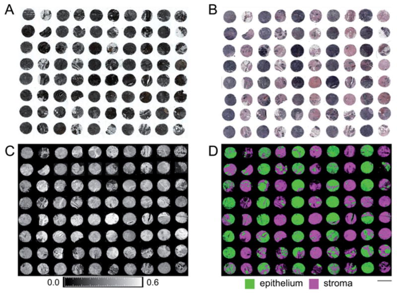
Two-class breast histology. (A) Minimal tissue and tumor characteristics are visible on unstained tissue. (B) Stroma and epithelium are visible on tissue stained with hematoxylin and eosin (H&E) dyes. (C) Image of tissue absorbance, as per color bar scale below the image, of unstained tissue at 3294 cm⁻¹ highlights differences in tissue, especially between stroma and epithelium. (D) Quantitative spectral data permits automated segmentation of stroma and epithelium, as noted by the color code below the image, without dyes or contrast agents. The scale bar represents the 1.5 mm diameter of a single core on this TMA.

Initial classification models are developed with spectral metrics to, first, segment epithelium and stroma and, second, segment the epithelium pixels as cancer or normal. As seen in Fig. 2A, spectral features for stroma and epithelium demonstrate substantial biochemical differences for these cell types. Average spectra are computed from manual labeling of epithelium (50 082 pixels) and stroma (140 100 pixels) on TMA cores in a calibration dataset with tissue from 40 different patients. A piecewise linear baseline is applied and a ratio is computed to the amide I absorbance at 1652 cm⁻¹ to normalize for tissue sample thickness. While scattering from tissue is well-known to affect spectra,^52–55 an analysis of the variance in tissue⁵⁶ shows that there is a significant fraction of the spectrum that can be useful for analysis using a simple baseline correction. More sophisticated models for spectral corrections^57–59 and physics-based methods^60,61 are being developed that can potentially provide more information and will likely improve our results here. In the baselined spectra we note especial differences within the fingerprint region, which contains many overlapping spectral features prevalent in tissue.⁶² The region includes symmetric PO₂ stretching and CO stretching vibrational modes at 1080 cm⁻¹, amide III protein modes within 1200–1338 cm⁻¹, CH₂ wagging at 1236 cm⁻¹, asymmetric PO₂ stretching at 1240 cm⁻¹, CH₂/CH₃ bending at 1400 cm⁻¹, asymmetric CH₃ bending at 1456 cm⁻¹, as well as the amide II vibrational modes within 1542–1556 cm⁻¹.⁶³ A broad amide A vibrational feature at 3294 cm⁻¹ (ref. 25) is also prominent, but we do not use the CH stretching region in our analysis due to additional strong variability arising from potentially residual paraffin. A comparison of the stroma and epithelium cell type spectra indicate that symmetric PO₂ vibrations in the DNA-rich tissue regions and CO stretching vibrations in secretory glycoproteins contribute a more significant relative absorbance in epithelium while asymmetric PO₂ stretching, amide III, and CH₂ wagging in the methyl side chains in collagen characterize the stroma IR spectrum. Clear spectral differences in these regions between epithelium and stroma indicate the potential for highly accurate classification.

Fig. 2.

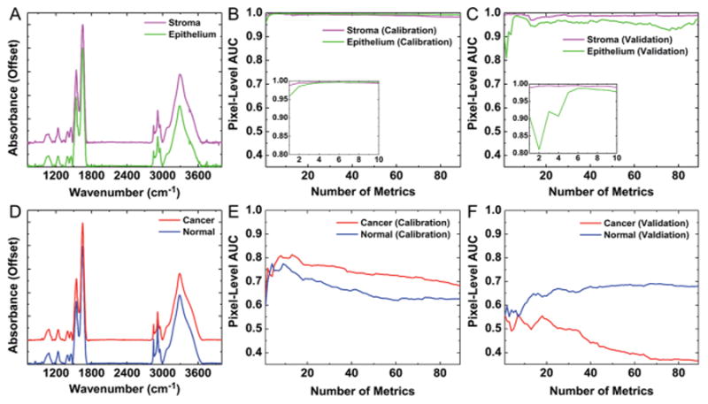
Automated histology and pathology using only spectral metrics. (A) Average spectra for stroma and epithelium demonstrate clear biochemical differences between these cell types. (B) Spectral metrics provide accurate histologic segmentation of stroma and epithelium with AUC values of ∼1 for each tissue class with only 6 metrics. (C) This classification is reproducible in validation on separate tissue samples. (D) Average spectra for cancer and normal epithelium indicate biochemical changes are less obvious in disease development. (E) ROC analysis indicates that spectral metrics demonstrate reduced discrimination in cancer and normal epithelium pixels with a maximum cancer pixel-level AUC of only 0.81. (F) Spectral metrics do not provide reproducible pathology discrimination, as demonstrated by a low cancer pixel-level AUC of 0.55 in validation samples.

As described in the methods section, a method for classification with spectral metrics provides accurate and reproducible differentiation of stroma and epithelium, as shown in Fig. 2B and C. This is demonstrated by the reproducible mean AUC value above 0.98 for both the calibration and validation TMA datasets with matched cancer and adjacent normal tissue samples from a set of 40 patients. Accurate histologic classification is accomplished with only 6 spectral metrics, as shown in the inset plots in Fig. 2B and C. Although each individual metric may not provide the same contribution to classification in the calibration and validation datasets, the AUC still reaches a maximum value in both datasets with the same six metrics. Notably, the classification contribution for individual metrics appears to vary more for epithelium than for stroma. This is reasonable, as collagen is a predominant component of breast stroma and has a distinct IR spectrum. Conversely, the IR spectrum for epithelium may vary more due to underlying physiologic conditions, for example between normal and different tumor regions, which would impact the performance of individual specific metrics in classification. It must be borne in mind that our model assumes two classes, but tissue is varied and the chemical diversity may not always fit the desired information model. Therefore, more than a few metrics are required to account for this diversity, compared to two-component polymeric systems for example.⁶⁴ A multi-feature classifier is advantageous to provide accurate and reproducible cell-type classification with spectral data.

Next, epithelium pixels were segmented into cancer and normal classes based on spectral metrics alone. The automated classification procedure was repeated with manually labeled epithelium from cancer (38 384) and normal (10 483) pixels as ground truth. From Fig. 2D, it can be seen that spectral differences are less obvious for cancer and normal epithelium. Although some small differences in absorbance are visible at 1400 cm⁻¹ and 1456 cm⁻¹, these distinctions are less clear than those between different cell types and may not facilitate efficient classification in the manner of epithelium–stroma with only spectral metrics. Indeed, the classification potential for spectral metrics is significantly lower for discriminating cancer and normal pixels, as evidenced by the cancer pixel-level AUC of 0.81 with eight spectral metrics in the calibration data (Fig. 2E) and 0.55 with the same eight metric classification model on validation data from the same patients (Fig. 2F). Notably, the metric contributions appear to vary even more between the calibration and validation datasets for the cancer class than for the normal class. This may indicate that spectral variation is greater for cancer epithelium pixels than normal epithelium pixels. In addition, the AUC appears to fall below 0.5 in validation for the cancer class when more than 33 metrics are included in the model. This analysis indicates that metrics during calibration optimization may have completely different properties for cancerous epithelium between different datasets, even when both datasets contain tissue from the same set of patients. Therefore, techniques to improve data quality such as computational noise reduction⁶⁵ or other image enhancement techniques⁶⁶ would likely provide only limited benefit for this classification problem. Given the poor performance and reproducibility of pixel-level classification, sample level analysis will also provide a low level of accuracy. Inaccurate classification results will also have wide sensitivity and specificity confidence intervals and AUC error estimates,^43,44 and will not be useful for tumor discrimination. These data may also indicate the need for more complex and better spectral features, a more sophisticated disease model going beyond the two-class model here or it may not be possible to perform this segmentation with IR imaging. Instead of pursuing complex models, corrections or computational-heavy methods to explore the potential of IR imaging, our goal was to develop a rapid protocol. Complex models and time-consuming calculations are not conducive to this. Hence, instead of mining the spectrum with more complex methods or applying spectral corrections, we chose to pursue an alternate method.

Classification with spectral and spatial metrics

The classification protocol with additional information that we propose and examine in this manuscript involves a two-step procedure outlined in Fig. 3. In Fig. 3A, the first step shows a spectral pixel-level segmentation of breast stroma and epithelium, which is highly accurate. In the second step, shown in Fig. 3B, a spatial information strategy is incorporated based on the epithelium–stromal segmentation. Computerized algorithms quantify epithelium content and arrangement with a technique termed spatial polling. Two algorithms for spatial polling are considered here. The first method involves TMA core-level spatial polling of a set of small tissue regions to obtain a diagnosis of cancer or normal for each individual core on a breast TMA. The second method involves pixel-level spatial polling of somewhat larger regions to obtain a diagnosis of cancer or normal for each individual pixel on a breast TMA. The advantages and challenges for each method are considered next prior to validation analysis. While there are many other spatial analyses methods available, we sought to develop a fast and robust method. Doubtless, more complicated methods can be developed and the ideas proposed here can be extended to other methods.

Fig. 3.

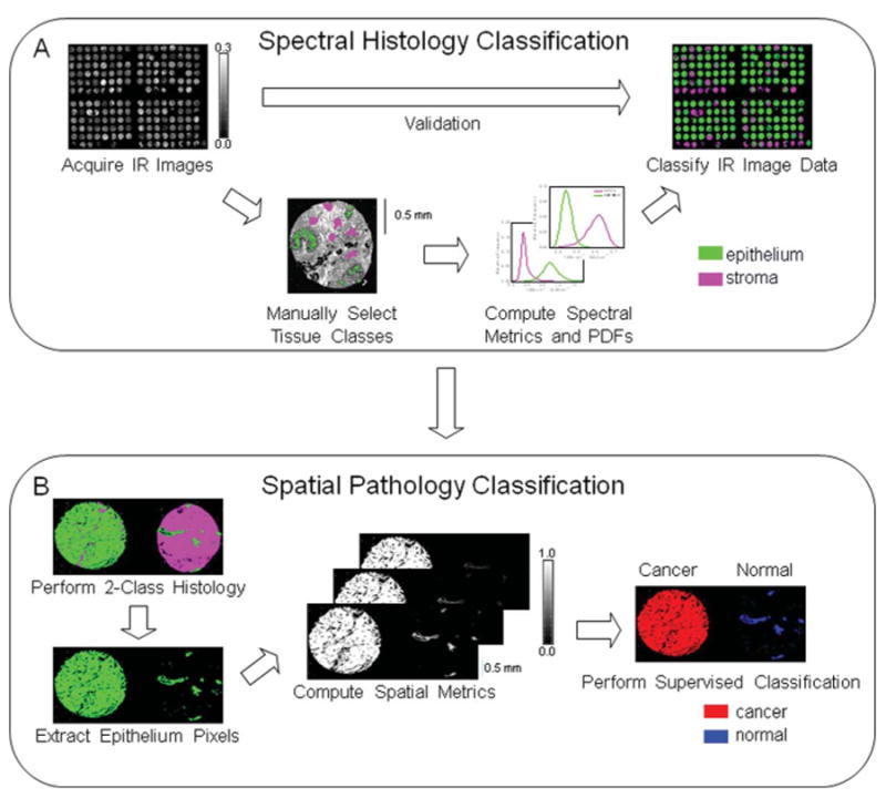
Development of automated breast histopathology with spectral and spatial data. (A) Spectral histologic classification was performed with supervised pattern recognition by acquiring an IR imaging dataset of multiple samples from a TMA and comparing images at frequencies of known biological significance with H&E staining, the current gold standard in pathology. A large set of pixels were manually selected to represent the two tissue classes [stroma, epithelium]. Frequency distributions for the two classes for each important spectral feature were computed and used to classify individual pixels. After calibration of the two-class histology model additional validation TMA dataset images were automatically classified without any operator intervention. (B) Spatial information from resulting histologic images was used for pathologic classification by extraction of epithelium pixels and computational pixel-level spatial polling. Resulting spatial metrics were used as the input for the supervised classification procedure, used previously for histology analysis, to segment epithelium pixels into cancer and normal classes.

First, TMA core-level spatial polling was conducted by dividing each TMA core into square boxes of specified dimensions (pixels). The percentage of boxes in each core with an epithelium fraction above a select threshold was computed. To minimize errors associated with inappropriate selection of a tissue region for tumor diagnosis, boxes containing no epithelium pixels were excluded from calculations. Square boxes sizes with pixel lengths of 1 × 1 to 12 × 12 were considered, and an 8 pixel (50 μm) box length was selected as an optimal size for tumor segmentation. As seen in Fig. 4A, cancer and normal cores are clearly separated at a wide range of epithelium fraction threshold values. A cutoff was selected for each epithelium threshold by the relationship

Fig. 4.

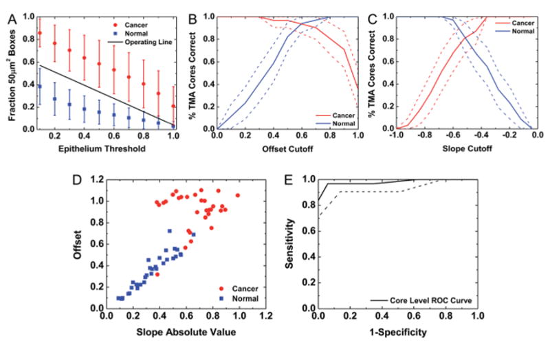
Tumor TMA core segmentation by spatial polling. (A) A TMA core was divided into 8 × 8 pixel (50 μm²) boxes and the fraction of boxes with epithelium content above a set of thresholds for each TMA core was computed. The mean value for cancer and normal classes was computed, and error bars represent standard deviation. An operating line was obtained for tumor TMA core classification. (B) A linear fit was calculated for each TMA core and the y-intercept offset cutoff for cancer detection was varied to assess classification sensitivity and specificity with this variable. (C) The slope cutoff for cancer detection was also varied to assess classification sensitivity and specificity with this variable. (D) A scatter plot of offset vs. slope absolute value for each TMA core demonstrates the contribution of each metric to tumor core identification. (E) The ROC curve indicates near-perfect tumor classification. The area between the dotted lines represents a 95% confidence region for the mean value.

$$\frac{d_{\mathrm{C}}}{d_{\mathrm{N}}}=\frac{{\sigma }_{\mathrm{N}}}{{\sigma }_{\mathrm{C}}}$$ (3)

where d_C is the distance of the cutoff from the mean of the cancer TMA cores, d_N is the distance of the cutoff from the mean of the normal TMA cores, σ_C is the standard deviation for cancer TMA cores, and σ_N is the standard deviation for normal TMA cores. A least squares linear fit was computed from the individual cutoff points for each epithelium threshold to determine the operating line for tumor detection in Fig. 4A.

A least squares linear fit with offset and slope values was also computed from the plots for the fraction of 50 μm² boxes above a selected epithelium threshold for each individual TMA core. Cutoff values for cancer detection for y-intercept offset (Fig. 4B) and slope (Fig. 4C) were varied and the sensitivity and specificity of tumor detection was evaluated. The plots in Fig. 4B and C indicate that both of these metrics simultaneously provide high sensitivity and specificity for tumor identification. To assess the potential of both of these metrics in a single classifier, the slope and offset were then plotted together (Fig. 4D) and an operating line was moved to perform ROC analysis and evaluate classification potential. From this plot, cancer cores appear to have a greater y-intercept offset and slope absolute value than normal cores. Although most cases can be distinguished by the offset variable alone, the slope variable appears to add additional information that is useful to achieve the best possible classification. An AUC of 0.98 ± 0.04 (95% CI) is achieved on the calibration TMA with 65 cores (31 cancer and 34 normal) using this technique (Fig. 4E). This method is highly sensitive to the overall morphology of the tumor and intervening stromal scales. Though the technique seems to work well, the method will underestimate regions where the tumor may be close to the edge. This will result in designation of pixels in sparse tumor regions or edges as non-cancerous and in a smaller spatial extent of tumor than present. Therefore, other techniques of spatial polling were evaluated for cancer classification.

A second spatial polling technique was considered to accomplish pixel-level cancer and normal epithelium segmentation. Again, the method was developed for histology classification with spectral metrics with a second-level set of spatial metrics to evaluate epithelium content and distribution. In this method, we propose a computational selection of boxes ranging in size from 16 × 16 pixels to 160 × 160 pixels. This range was selected to evaluate regions varying in size from the approximate mean diameter of a normal breast duct⁶⁷ to an area approaching the size of a typical TMA core. A somewhat larger area is required for the pixel-level spatial polling than the core-level spatial polling from Fig. 4 because the metrics are computed separately for each individual pixel and are not averaged over an entire TMA core. The fraction of pixels in each box classified as epithelium was determined, and an average and standard deviation for the epithelium fraction was computed for each pixel from all boxes of a given size containing that pixel. These pixel-level computations were stored in an image metric vector with a format similar to the spectral metric vector used for histology classification. To evaluate the relative classification potential for spatial metrics, all pixels labeled as epithelium by histology classification considered as ground truth information with 1 030 376 cancer pixels and 181 350 normal pixels. Epithelium pixels were divided into cancer and normal classes by applying the same automated classification algorithm used to segment stroma and epithelium pixels but now with spatial metrics. Pixel-level ROC analysis was then performed for each class. Cancer and normal classification images were obtained at the operating point for each class where the difference between the fraction of pixels correctly and incorrectly classified was maximized. TMA core-level tumor identification was then accomplished by selecting an appropriate fraction of epithelium pixels on a TMA core labeled as cancer in the classification image as a threshold to diagnose the entire TMA core as cancer. This threshold was varied to produce an ROC curve to evaluate overall TMA core-level cancer classification potential.

To determine an appropriate region for pixel-level spatial polling, a single metric cancer and normal pixel-level classification model was developed for each box size metric and the area under the ROC curve (AUC) was plotted separately for each classifier. The plot for AUC vs. box size for 16 × 16 pixels to 160 × 160 pixels is displayed in Fig. 5A. The plot and images in this figure demonstrate that tumor identification is strongly influenced by the size of the spatial polling region. When a very small region of 16 × 16 pixels is considered, only a few cancer epithelium pixels are correctly classified and some normal pixels are misidentified as cancer (Fig. 5B). Clearly, this low sensitivity and specificity is not suitable for tumor detection. Therefore, a larger region must be considered for reasonable tumor identification. When a region greater than 48 × 48 pixels is considered the core-level classification AUC appears to plateau at a high value around 0.95 ± 0.06 (95% CI). A classified image for a spatial metric in this range with a box size of 80 × 80 pixels (Fig. 5C) indicates that a good separation of cancer and normal epithelium is achieved with some pixels labeled as cancer in 29 of 31 tumor TMA cores and normal pixels labeled as cancer in only 3 of 34 adjacent normal TMA cores. The core-level AUC begins to decline at a box size of 128 × 128 pixels, primarily due to a reduced sensitivity to small tumor regions in cancer TMA cores. A classified image for spatial polling with a box size of 160 × 160 pixels indicates that no pixels are labeled as cancer in 6 of 31 tumor TMA cores (Fig. 5D). These cores have small or more diffuse tumor regions that may not be detected when only a relatively large area is considered by spatial polling. This loss in classification accuracy with spatial polling at large regions indicates that both epithelium structure and content are important for TMA core-level tumor discrimination, as a classifier based only on epithelium content would likely produce asymptotic behavior after obtaining a maximum AUC value. Conversely, pixel-level classification accuracy increases at a relatively constant rate as the box size increases and levels off as the area considered begins to approach the size of a 1.5 mm diameter TMA core. The pixel-level classification AUC begins to reach a plateau at a box size of 120 × 120 pixels. For a pixel at the center of the TMA core with each 750 × 750 μm² box containing this pixel included a total region of approximately 2.25 mm² is actually considered by spatial polling, which encompasses the entire TMA core. Therefore, the pixel-level classification AUC approaches the core-level AUC when box sizes above 120 × 120 pixels are employed for spatial metric computation. Pixel-level and core-level classification do not follow the same trend for AUC vs. box size because different TMA cores have dramatically different numbers of epithelium pixels. Therefore, not all epithelium pixels are weighted equally in core-level ROC analysis.

Fig. 5.

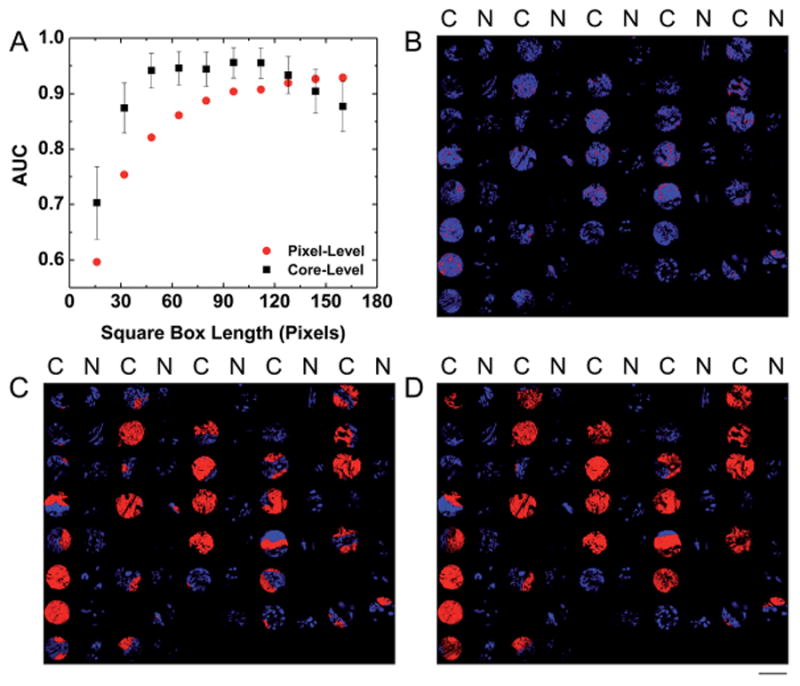
Automated pathology with spatial metrics. (A) A plot of AUC vs. square box length in pixels indicates that accurate TMA core-level classification can be achieved at a range of box sizes and that pixel-level classification becomes more accurate as the box size increases. Error bars for the core-level AUC values represent standard error. (B) A classified image from a 16 × 16 pixel box size indicates low sensitivity when only a small spatial neighborhood is considered. Red represents pixels classified as cancer and blue represents pixels classified as normal. The notation [C, N] denotes [cancer, normal] samples as judged by pathologist review. (C) A classified image from an 80 × 80 pixel box size indicates increased sensitivity with high specificity when a larger spatial neighborhood is considered. (D) A classified image from a 160 × 160 pixel box size (1000 μm²) indicates reduced sensitivity when a spatial area larger than the tumor area in some TMA cores is considered. The scale bar represents a 1.5 mm diameter of an individual core on this TMA.

While this simple approach yields encouraging results, multiple scales of spatial classification and morphologic diversity were evaluated by adding additional types of metrics and combining metrics from different box sizes. Metrics of the mean and standard deviation of the fraction of pixels classified as epithelium in all boxes of a selected size containing a given pixel were computed for box sizes ranging from 4 × 4 pixels (25 μm²) to 160 × 160 pixels (1000 μm²). This range was selected to evaluate areas that contain only a few cells to an entire TMA core. These metrics were combined to obtain an 80-metric image vector with fraction mean and standard deviation metrics for a square box length of pixels 4,8,16 and so on up to 160. Cancer TMA cores are expected to have higher values for fraction mean metrics since a large mass of epithelium often signifies a tumor. Conversely, normal TMA cores are expected to have higher values for fraction standard deviation metrics since normal breast tissue contains ducts and lobules lined with a thin layer of epithelium. The metrics were sorted by the average estimated error from frequency distributions and used to build a classifier with 1 metric, 2 metrics, 3 metrics, and so on until all 80 metrics were included. A total of 80 classifiers were built, and ROC analysis was performed and an AUC value was computed for each classifier. The ΔAUC value was computed with the addition of each spatial metric and the metrics were re-sorted to select a set that provides optimal classification with a minimal number of spatial metrics. To evaluate the contribution of spatial metrics when only a smaller area of tissue is considered, this classification optimization was repeated with a smaller 40-metric vector containing fraction mean and standard deviation metrics for box sizes ranging from 4 × 4 pixels (25 μm²) to 80 × 80 pixels (500 μm²).

Pixel- and core-level ROC analysis for each classifier indicates that adding additional mean and standard deviation metrics has a varying impact on AUC. From the 40-metric vector with a maximum 80 × 80 pixel region an optimal classifier was obtained with 2 spatial metrics: an 80 × 80 pixel (500 μm²) mean and a 16 × 16 pixel (100 μm²) standard deviation. In Fig. 6A, cancer and normal pixel-level ROC curves are compared before and after the addition of the standard deviation spatial metric. The pixel-level cancer AUC value is increased from 0.87 to 0.9 and the pixel-level normal AUC value is decreased from 0.91 to 0.88 to provide a minimal overall increase of 0.001 in mean AUC with the addition of the standard deviation metric. The core-level AUC value is reduced from 0.94 ± 0.06 (95% CI) with the single metric classifier with an 80 × 80 pixel mean (Fig. 6B) to 0.92 ± 0.07 (95% CI) with the two metric classifier with an 80 × 80 pixel mean and a 16 × 16 pixel standard deviation (Fig. 6C). While this change is not statistically significant, it does indicate that these additional standard deviation metrics may not be independently beneficial for core-level tumor identification. The discrepancy between pixel and core level classification is explained by examining TMA classified images and the shape of the ROC curve with and without the additional spatial metrics. When the mean fraction metric is considered alone, on most normal cores no pixels are classified as cancer. However, the addition of the standard deviation metric appears to increase the number of pixels classified as cancer on both tumor and normal TMA cores due to spatial heterogeneity. This small increase in non-specific pixels classified as cancer in normal TMA cores is responsible for the observed reduction in specificity on the core-level ROC curve and corresponding reduction in AUC with the addition of the standard deviation spatial metric.

Fig. 6.

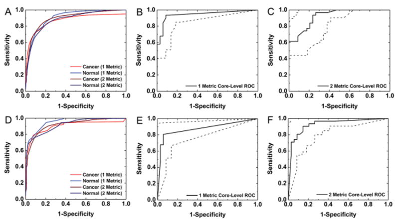
Classification with multiple types of spatial metrics. (A) ROC analysis for multiple classification models for pixel-level cancer and normal segmentation using metrics computed from a box size range of 4 × 4 pixels to 80 × 80 pixels demonstrates some improvement in pixel-level cancer sensitivity with multivariate classification. (B) ROC analysis for core-level classification with a single metric of mean fraction for an 80 × 80 box indicates accurate overall tumor identification. (C) Core-level specificity is somewhat reduced with the addition of a standard deviation spatial metric for this 80 × 80 box size classifier. (D) ROC analysis for univariate and multivariate classification models for pixel-level cancer and normal segmentation using metrics computed from a box size range of 4 × 4 pixels to 160 × 160 pixels demonstrates some improvement with multivariate classification. (E) ROC analysis for core-level classification with a single mean fraction metric for a 160 × 160 box indicates reduced sensitivity in tumor detection. (F) Core-level sensitivity is improved with the addition of a standard deviation metric to this 160 × 160 box size spatial polling classifier. The areas between the dotted lines on the core-level ROC curves represent 95% confidence regions.

Multi-level classification may provide advantages for core-level tumor detection when a larger tissue area is considered. When the entire 80-metric vector was employed to build an optimal classification model, 3 metrics were selected. These metrics include fraction mean metrics for box sizes of 160 × 160 pixels (1000 μm²), 152 × 152 pixels (950 μm²), and 148 × 148 pixels (925 μm²). These additional metrics provide a minimal increase from 0.906 to 0.908 in pixel-level cancer AUC, from 0.952 to 0.953 in pixel-level normal AUC, and from 0.929 to 0.930 in pixel-level overall mean AUC. These increases in AUC are smaller than those observed when the smaller 80 × 80 pixel region was considered in spatial polling because the initial pixel-level AUC values with the single 160 × 160 mean metric classifier are greater, and may approach the maximum AUC value that can be attained with the information in these spatial metrics. The estimated core-level AUC was also increased by 0.01 from 0.88 ± 0.09 (95% CI) to 0.89 ± 0.08 (95% CI). The width of the confidence interval was reduced due to the increase in AUC,⁴³ even though the same set of 31 cancer and 34 normal samples were used for both analyses. However, the forward metric selection procedure employed in this classification model is not exhaustive and does not consider all potential metric combinations, and this selected model may not be the only useful model for classification with this spatial polling region.

To understand the influence of mean fraction metrics of different sizes, a classification model was built with the 160 × 160 pixel mean and 16 × 16 pixel standard deviation spatial metrics. With this classification model, the cancer pixel-level AUC was increased from 0.906 to 0.915, the normal pixel-level AUC was reduced from 0.95 to 0.92, and the mean pixel-level AUC was reduced from 0.93 to 0.92. The pixel-level ROC curves in Fig. 6D indicate that these changes in AUC with the multivariate classifier are not substantial for pixel-level cancer classification. Conversely, the core-level AUC was increased from 0.88 ± 0.09 (95% CI) with a single metric classifier with a 160 × 160 mean fraction (Fig. 6E) to 0.93 ± 0.07 (95% CI) with a 2 metric classifier with a 160 × 160 mean fraction and a 16 × 16 standard deviation (Fig. 6F). Although this increase is not statistically significant due to the limited number of samples included in the training analysis, the new classifier does appear to provide a substantial benefit for core-level tumor classification when large regions are considered. This change in AUC is reflected in the classified images and shape of the ROC curve. As noted earlier, classification with a single 160 × 160 fraction mean metric results in 6 missed tumors out of 31 total cancer TMA cores in the calibration dataset. This limitation in sensitivity is reflected in the TMA core-level ROC curve with this single metric classifier in Fig. 6E. When the optimal multivariate classifier with this metric is employed, pixels are labeled as cancer in 30 out of 31 cancer TMA cores. This increase in sensitivity is reflected in the multivariate core-level ROC curve in Fig. 6F and results in the increased observed AUC value. A previous study of 432 breast ducts with necrosis from 26 cancer patients and 520 ducts from 26 normal autopsy samples indicated that the ducts from advanced tumors with intraductal necrosis were rarely smaller than 240 μm in diameter while ducts from normal samples were rarely larger than 180 μm in diameter.⁶⁷ Therefore, this spatial metric may provide important information for pixel-level tumor discrimination at a single duct scale. As indicated in Fig. 5, a spatial metric computed from this spatial area alone does not provide accurate tumor discrimination. However, when it is combined with spatial polling over larger areas of tissue it may provide useful additional information for tumor classification.

After consideration of a broad range of spatial regions and multiple combinations of spatial metrics, a single spatial polling classifier was selected for extensive validation analysis. Although a maximum pixel-level AUC is only achieved by spatial polling over areas approaching the size of a TMA core, optimal core-level classification can be achieved with consideration of a much smaller area. Since high density validation TMAs contain cores of diameter 1 mm or smaller, TMA core-level validation analysis was performed with the smallest region to produce an estimated core-level AUC of at least 0.95 on the calibration dataset. Therefore, a spatial polling region of 52 × 52 pixels (325 μm²) was selected for farther evaluation. This area is reasonable, as a study of 1285 breast ducts from 26 breast ductal carcinoma patients found a mean diameter of 349 μm.⁶⁷ Therefore, a region of this size with a high fraction of epithelium should encompass a tumor. Models with this metric were considered but rejected when the TMA core-level AUC was not increased.

Tumor classification validation and sample size analysis

The expected AUC and desired confidence interval half-width were considered in selecting the appropriate sample size for validation. For a binomial problem of unknown sample size with 2 classification options, e.g. cancer and normal, the AUC variance can be estimated as

$${\sigma }^2\left(\theta \right)=\theta \left(1-\theta \right)$$ (4)

where θ is the predicted AUC value.⁶⁸ This variance can be employed with an acceptable half-width for a confidence interval (L) and a given total sample size (n) to calculate a corresponding z-score by the equation

$$z_{\alpha /2}=L\sqrt{\frac{n}{\theta \left(1-\theta \right)}}\left(\text{ref}.68\right).$$ (5)

The p-value associated with the computed z-score is then obtained from tabulated z tables or software packages. In this manner, the z-score will increase linearly with L and the corresponding p-value will increase until it approaches a value of one. This p-value represents the probability that the true AUC is greater than or equal to the lower bound of the confidence interval. For example, for an AUC of 0.95 ± 0.02, a p-value of 0.95 would indicate that an AUC of at least 0.93 will be obtained in 95 out of 100 validation studies with the similar sampling. Therefore, a confidence of 0.95 can be assigned to the interval obtained in that study. The confidence assigned to an AUC value depends upon both the estimated AUC value θ and the sample size n. This is reflected in eqn (5), in which the z_α/2 score and corresponding p-value increase with n and decrease with θ. This is expected, since populations with less overlap in metric distribution will be more easily separated and studies with a larger sample size will produce a smaller standard error. This trend is reflected in Fig. 7, where confidence increases with sample size for a given θ until it reaches a maximum value near 1. In this plot an interval half width L of 0.02 is assumed for all z_α/2 and confidence calculations. If the expected AUC value is known from calibration studies, an appropriate sample size n can be selected where the p-value begins to approach 1. For an estimated θ of 0.95, the confidence levels off near a value of 1 with a sample size of n = 700. Therefore, our methods predict the number of samples required for definitive validation in addition to developing the protocol itself. The issue of sample size has received some attention as it is a critical aspect of the development of protocols. While at least one previous study examined the effect of sample size theoretically,⁶⁹ the integration of classification and statistical validation can be jointly accomplished in the manner above. The combination of spectral histology and spatial polling for tumor identification translates effectively to independent validation samples, as demonstrated by the consistent high AUC values for validation. Although the algorithm is trained exclusively on TMA cores of 1.5 mm in diameter, it translates directly to smaller cores of 1 mm diameter. We have further tested the samples on TMAs that contained cores of sizes as small as 1 mm as well as surgical resections. A detailed study of the validation and the limitations of this study is beyond the scope here and will be analyzed in a future report.

Fig. 7.

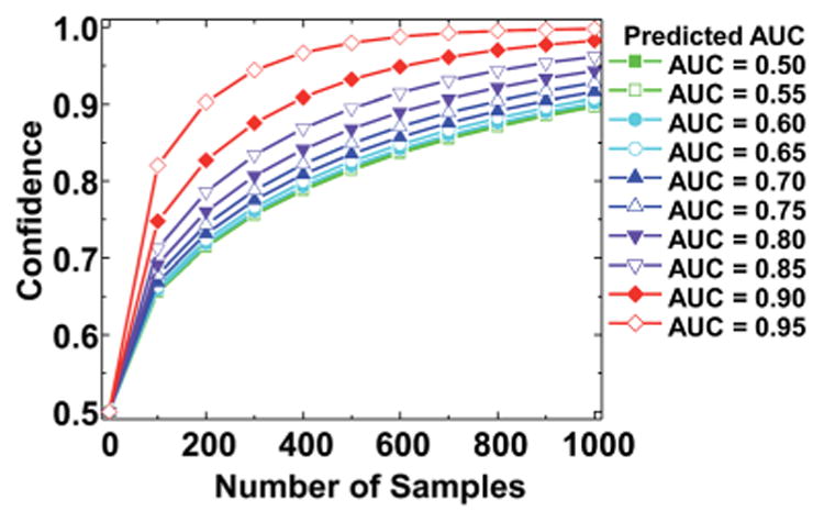
Prediction of sample size for a potential validation study. Confidence in the AUC value shows a variation with the value of the AUC and the sample size for an interval of half-width 0.2 at a range of AUC values. Confidence increases with both AUC and sample size and the precise sample size needed can be read from the chart.

Applications for clinical translation

To implement this technique efficiently in a clinical setting, rapid data acquisition and analysis is necessary as classification of IR datasets can be performed in a matter of minutes. The “standard” data collection parameters of 4 cm⁻¹ spectral resolution, 2 scans per pixel, and a 6.25 μm pixel size dictate an acquisition time of at least 1.5 hours to collect data for a 1.5 mm TMA core. These parameters, in our experience, provide an excellent trade-off between data quality and time of acquisition while providing accurate biomedical segmentation for other tissues. As breast tumors are normally evaluated in a clinical setting on much larger biopsy surgical resections, these data collection parameters are not reasonable for clinical implementation with conventional IR imaging instrumentation. One route to increasing the rate of data acquisition can be to reduce the required signal to noise ratio (SNR) or coarsen spectral resolution from these levels.⁷⁰ From the trading rules for IR spectroscopy, data collection time decreases linearly with spectral resolution and in quadrate with SNR,⁷¹ trends that also hold for IR imaging.^72,73 In addition, a different hardware configuration using a FPA detector can be employed for rapid data acquisition.^74,75 The potential for each of these options is evaluated next in this manuscript to assess the impacts on single pixel spectra, spectral histology classification and spatial pathology classification. Qualitative image evaluation and quantitative ROC analysis were employed to determine the classification potential with reduced spectral quality and detail in IR image datasets.

In practice, a reduction in SNR can be accomplished by decreasing the number of scans per pixel required for data acquisition. To evaluate the potential of classification on high noise data, random Gaussian noise was added to one validation dataset and spectral and spatial classification for the original dataset and the dataset with noise added were compared to assess spectral histology and spatial pathology classification. The RMS noise for background pixels was estimated as 0.001 before adding noise and 0.016 after adding noise. When individual pixel spectra without and with added noise were compared, the added noise clearly obscured many important features within spectra, as shown in Fig. 8A. This is particularly apparent in the fingerprint region, which contains many of the key metrics used in the histology model to segment stroma and epithelium. This loss in spectral quality is reflected in the histology classification ROC analysis. In Fig. 8B, it can be seen that the AUC value for stroma is reduced from 0.99 to 0.95 and the AUC value for epithelium is reduced from 0.98 to 0.88 with added noise. Since a large number of pixels (30 140 stroma and 20 019 epithelium) are used in validation ROC analysis these changes are statistically significant. Notably, the epithelium AUC appears to be more adversely effected by noise than the stroma AUC. A comparison of classified histologic images before and after the addition of noise in Fig. 8E and F, respectively, indicates that randomly distributed epithelium pixels are misclassified as stroma. This reduction in epithelium sensitivity is the primary cause for the drop in the epithelium AUC value. This may be due to the epithelial spectra, consisting of a small set of broadly distributed peaks, leading to a higher apparent absorbance that starts to overlap with the stromal values. Conversely, the stroma spectrum appears more similar to collagen, with a larger set of more overlapping narrow peaks and an increase in values does not affect classification and a decrease in values folds into the tails of the lower noise distributions. By adding random noise, the epithelial spectra become more similar to stromal spectra, which would lead to random misclassifications of epithelium pixels as stroma. Since these misclassification events are random instead of systematic, both histology class images correspond reasonably well with H&E staining (Fig. 8D).

Fig. 8.

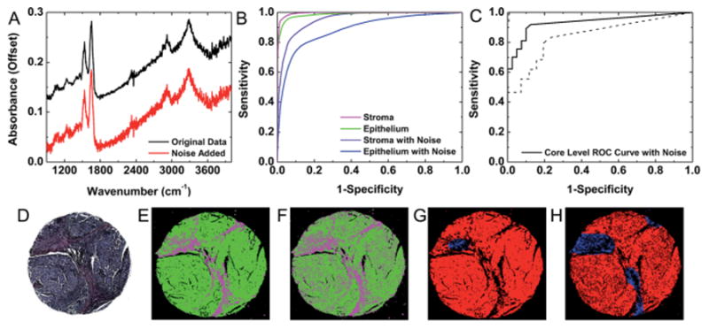
Classification with reduced SNR. (A) A single pixel spectrum (epithelial) from the original dataset and the dataset with noise added demonstrates reduced visibility of spectral features, particularly in the fingerprint region. (B) Pixel-level segmentation accuracy of stroma and epithelium is decreased in high-noise data, but reasonable cell-type classification is still possible. (C) ROC analysis indicates that reasonable core-level tumor classification is possible with the addition of noise to the dataset. The area between the dotted lines represents bounds for a 95% confidence region. (D) H&E staining, (E) histology classification and (F) pathology classification by spatial polling on the original dataset indicate that this sample contains a dense invasive epithelial tumor. (G) This core classification from the dataset with noise added indicates some reduction in epithelium detection. (H) Tumor detection is also somewhat less sensitive in the core with noise added.

Conversely, the core-level tumor diagnosis AUC value only decreased from 0.97 ± 0.04 (95% CI) for the original dataset to 0.93 ± 0.06 (95% CI) for the dataset with added noise. As this change is not statistically significant, spatial polling can be performed on low SNR data without a statistically significant loss in classification potential. The ROC curve in Fig. 8C indicates that reasonable cancer detection sensitivity and specificity are achieved in the high noise dataset. A comparison of the classified images before and after the addition of noise indicates that the loss in AUC is due to a reduction in sensitivity, which may be a concern for cancer classification. However, most of this loss in sensitivity occurs near epithelium boundary pixels, as evidenced by the classification images to distinguish cancer (red) before and after adding noise in Fig. 8G and H, respectively. Therefore, large tumor regions can still be readily identified in high noise datasets.

Next, spectral resolution was evaluated for its effect on the spectral and spatial classification potential. Previous studies have demonstrated by simulation that a coarser spectral resolution of 16 cm⁻¹ can be sufficient for histology classification.^70,76,77 This could potentially decrease data collection time by a factor of 64 due to the dual benefit of collecting fewer points and more light throughput per spectral element. Hence, we tested our approach for histology and pathology classification on two datasets acquired at a 16 cm⁻¹ spectral resolution. The first dataset was acquired at 4 cm⁻¹ and 16 cm⁻¹ spectral resolutions on a 16 × 2 linear array detector and then at 16 cm⁻¹ on a separate IR imaging instrument with a 128 × 128 FPA detector. The second dataset was acquired at only a 16 cm⁻¹ spectral resolution on the linear array detector. This dataset was employed for validation of classification from rapid image acquisition. A spectrum from a pixel (stromal) was first examined from an image collected at 4 cm⁻¹ with the linear array detector, at 16 cm⁻¹ with the linear array detector, and at 16 cm⁻¹ with the FPA detector in Fig. 9A. Since biomedical spectra are typically complex mixtures, many of the broad spectral features remain apparent at the coarser spectral resolution. However, some finer spectral features apparent in the 4 cm⁻¹ spectrum are less obvious in the 16 cm⁻¹ resolution spectra. Notwithstanding, the 16 cm⁻¹ spectra collected with the linear and focal plane array detectors appear to provide similar information. These observed spectral differences, however, are not important in themselves and need to be evaluated in the context of histologic classification. Classification of an IR image collected at a 4 cm⁻¹ spectral resolution in Fig. 9D provides similar information to H&E staining in Fig. 9C. However, when classification is repeated on images collected at a 16 cm⁻¹ spectral resolution with a linear array detector (Fig. 9E) and a FPA (Fig. 9F) there appears to be a bias towards epithelium classification. This may be attributed to the reduced definition of some stroma spectral features associated with collagen in the spectra collected at a 16 cm⁻¹ resolution. Nevertheless, in many cores the observed classification of images collected at a 4 cm⁻¹ and a 16 cm⁻¹ spectral resolution is relatively similar. The robust nature of the cell type classification can be attributed to the types of metrics employed in classification. The peak heights and ratios are relatively consistent as long as the full width at half maximum (FWHM) value remains unchanged. The peak area and center of gravity metrics are also not highly impacted by small changes in peak shape or location.⁷⁰ Finally, many classified TMA cores appear similar when acquired at a 16 cm⁻¹ spectral resolution with either the linear array or the FPA detector. Therefore, the spectral classification technique is broadly applicable across different spectral resolutions and IR imaging instruments.

Fig. 9.

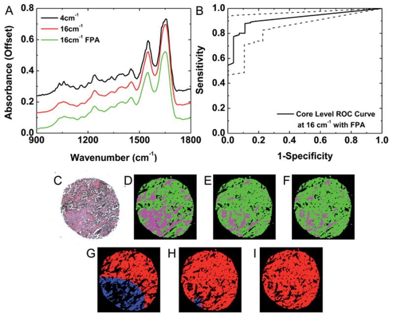
Classification with a linear array and focal plane array detector with low resolution data. (A) A single-pixel stroma spectrum from images acquired at a 4 cm⁻¹ spectral resolution with a linear array detector, 16 cm⁻¹ spectral resolution with a linear array detector, and a 16 cm⁻¹ spectral resolution with a FPA detector indicate some spectral changes associated with spectral resolution but minimal spectral variation associated with the detector. (B) ROC analysis indicates that accurate core-level classification is achieved at a 16 cm⁻¹ spectral resolution with a FPA detector. (C) An epithelium tumor is detected by conventional H&E staining. (D) An IR image of a single TMA core collected at a 4 cm⁻¹ spectral resolution with a linear array detector demonstrates epithelium (green) and stroma (magenta) segmentation that is consistent with H&E staining. (E) An IR image of this TMA core collected at a 16 cm⁻¹ spectral resolution with a linear array detector demonstrates some additional pixels classified as epithelium. (F) An IR image of this TMA core collected at a 16 cm⁻¹ spectral resolution with a FPA detector demonstrates similar classification to the image collected at 16 cm⁻¹ with the linear array detector. (G) Pixel-level classification segments the epithelium pixels as cancer (red) or normal (blue) from the 4 cm⁻¹ histology classified image. (H) Somewhat more epithelium pixels are identified as cancer from the 16 cm⁻¹ image collected with the linear array. (I) The 16 cm⁻¹ image collected with the FPA detector provides similar tumor identification as the image collected with the linear array detector.

Despite some differences in spectral histology, core-level pathology classification appears to be reproducible across different spectral resolutions and IR imaging instruments. Spectral histology images were classified by spatial polling to segment epithelium pixels as cancer or normal. Observed differences in pathology classification of the IR images collected at 4 cm⁻¹ (Fig. 9G), at 16 cm⁻¹ (Fig. 9H), and at 16 cm⁻¹ with the FPA detector (Fig. 9I) follow the pattern of observed differences in histology classification, with the epithelial pixels in the section with more stroma from the 4 cm⁻¹ IR image misclassified as normal due to the increased stromal content. In addition, minimal differences were observed in cancer identification between the 16 cm⁻¹ images collected with different instruments. The square pixel size for the FPA is somewhat smaller, with a length 5.5 μm instead of 6.25 μm. Therefore the estimated box area on the FPA image is 286 × 286 μm², which is somewhat smaller than the 325 × 325 μm² area considered on all other images collected with the linear array detector. However, the core-level tumor detection ROC analysis in Fig. 9B on the image acquired with the FPA still appears to be highly accurate, with an AUC of 0.92 ± 0.04 (95% CI). Classification at a 16 cm⁻¹ spectral resolution is confirmed on an additional validation TMA with 180 samples. Pixel-level ROC analysis for stroma and epithelium histology segmentation in Fig. 10A provides quantitative evidence of reproducible histology, with an AUC of 0.93 for epithelium and 0.96 for stroma. The small reduction in AUC for epithelium is due to a loss in specificity, which confirms the previous observation that some stromal pixels are mislabeled as epithelium. However, the histology AUC values for both classes are still acceptable. Next, core-level cancer detection ROC analysis was performed to assess tumor identification. From the plot in Fig. 10B, high sensitivity and specificity were achieved on this dataset with an AUC of 0.95 ± 0.03 (95% CI). These results indicate that data collection at a coarser 16 cm⁻¹ spectral resolution is sufficient to achieve automated cell type classification and tumor detection in breast tissue.

Fig. 10.

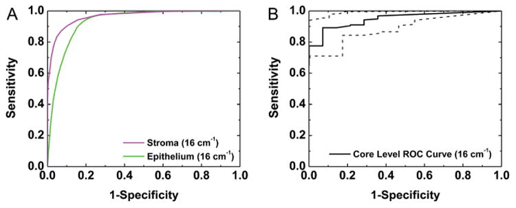
Validation at a course spectral resolution. (A) Pixel-level segmentation of epithelium and stroma is demonstrated on a 180 patient TMA collected at a 16 cm⁻¹ spectral resolution. (B) ROC analysis indicates that accurate core-level cancer detection is also achieved on this dataset.

To achieve cost-effective imaging in a clinical setting, sample preparation expenses must also be minimized. All evaluations to this point in this study have been performed on images collected by light transmission, which generally provides the best quality datasets. Other studies have reported using glass slides,⁷⁸ which involve a trade-off between practicality and reduction in spectral wavelength bandpass, or reflective glass slides, which require transflection model imaging. Another alternative is to use attenuated total reflection mode sampling,⁷⁹ which can offer higher spatial resolution⁸⁰ but requires good contact with the sample that can be cumbersome for translation. To be compatible with clinical workflow as well as obtain the full spectrum, we chose to evaluate the approach using thin sections deposited on reflective glass slides. An adjacent section of the calibration TMA was placed on a reflective slide and images were acquired by light transflection with all other data collection parameters the same as transmission imaging. Transflection induced changes in spectra are well known,^81,82 but there is emerging evidence to demonstrate effective classifications despite these effects.⁸³ Spectral histologic classification was again performed to segment stroma and epithelium from this data set. Examination of classified images of a TMA core collected by transmission (Fig. 11D) and transflection (Fig. 11E) demonstrate similar classification in both datasets and reasonable correlation with H&E staining (Fig. 11C). Pixels were then labeled on the same cores as the calibration TMA, with 140 899 stroma pixels and 50 393 epithelium pixels manually annotated as a gold standard. Pixel-level histology ROC analysis was then performed to provide a quantitative assessment of the classification accuracy. An AUC of 0.99 was obtained for epithelium and 0.98 was obtained for stroma in transflection datasets. From the pixel-level AUC plots in Fig. 11A a minimal reduction in AUC is observed between the transmission and transflection images. These small differences can likely be attributed to optical effects and changes in SNR due to the double-pass nature of the measurement transflection imaging. Likewise, transmission and transflection images produce similar tumor identification. Pathology classified images for a single TMA core collected by transmission (Fig. 11F) and transflection (Fig. 11G) demonstrate that most epithelium pixels are correctly labeled as cancer in both images. This observation is confirmed by core-level ROC analysis on 75 samples in Fig. 11B with an AUC of 0.93 ± 0.06 (95% CI). While slightly lower than the transmission AUC of 0.95 ± 0.06 (95% CI), these results are not statistically different. Therefore, accurate tumor identification is possible by transflection image, spectral histology classification, and spatial pathology classification. Since our analysis is not based on complicated spectral analysis, rather on a simple spectral and spatial analysis, we anticipate that small changes in known confounding variables such as sample thickness will not have a significant impact. However, a comprehensive test needs to be conducted to quantify the effect, if any, of such changes.

Fig. 11.

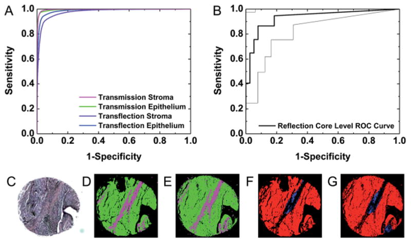
Validation of transflection-mode imaging data. (A) Pixel-level ROC analysis indicates similar histologic classification accuracy is achieved in transmission and transflection images. (B) Core-level ROC analysis indicates that transflection images can be accurately classified to identify tumors. The area between the dotted lines represents a 95% confidence region. (C) H&E staining, (D) transmission histology, and (E) transflection histology images demonstrate similar cell-type segmentation. Green labels epithelium and magenta labels stroma as in previous images. (F) Transmission and (G) transflection images demonstrate similar patterns of tumor detection. Red labels cancer and blue labels normal epithelium pixels, as noted previously.

Conclusions

Combining FT-IR imaging, spectral histology classification, and spatial pathology classification is demonstrated to provide automated, accurate, and reproducible tumor identification. Each pixel is first labeled as stroma or epithelium using spectral recognition at the single pixel level; subsequently, epithelium pixels are labeled as cancer or normal by spatial polling based upon epithelium content and distribution. Robust classification is demonstrated in a definitive validation study. Options are considered for efficient clinical translation, including classification of data with increased noise or reduced spectral resolution. Tumor classification is also demonstrated on images collected with a FPA detector and on inexpensive reflective glass slides. The data demonstrate that a practical protocol for rapid breast cancer identification is possible and the various tradeoffs in speeding up or reducing costs for clinical translation. Validation of this protocol and advances in instrumentation for rapid data acquisition can lead to a practical solution for breast cancer detection on biopsy samples.

References

- 1.Howlader N, Noone AM, Krapcho M, Garshell J, Miller D, Altekruse SF, Kosary CL, Yu M, Ruhl J, Tatalovich Z, Mariotto A, Lewis DR, Chen HS, Feuer EJ, Cronin KA, editors. SEER Cancer Statistics Review, 1975–2012. National Cancer Institute; Bethesda, MD: Apr, 2015. http://seer.cancer.gov/csr/1975_2012/ based on November 2014 SEER data submission, posted to the SEER web site. [Google Scholar]
- 2.Chagpar AB, McMasters KM. J Surg Res. 2007;140:214–219. doi: 10.1016/j.jss.2007.01.034. [DOI] [PubMed] [Google Scholar]
- 3.Thomson Reuters In-Patient and Out-Patient Views Market-Scan Database. 2008 [Google Scholar]
- 4.Parker SH, Burbank F, Jackman RJ, Aucreman CJ, Cardenosa G, Cink TM, Coscia JL, Eklund GW, Evans WP, Garver PR, Gramm HF, Haas DK, Jacob KM, Kelly KM, Killebrew LK, Lechner MC, Perlman SJ, Smid AP, Tabar L, Taber FE, Wynn RT. Radiology. 1994;193:359. doi: 10.1148/radiology.193.2.7972743. [DOI] [PubMed] [Google Scholar]
- 5.Carter D. Interpretation of Breast Biopsies. 4th. Lippincott Williams & Wilkins; Philadelphia: 2004. pp. 37–50. [Google Scholar]
- 6.Hatmaker AR, Donahue RMJ, Tarpley JL, Pearson AS. Am J Surg. 2006;192(5):e37. doi: 10.1016/j.amjsurg.2006.08.028. [DOI] [PubMed] [Google Scholar]
- 7.Simunovic M, Gagliardi A, McCready D, Coates A, Levine M, DePetrillo D. Can Med Assoc J. 2001;165(4):421. [PMC free article] [PubMed] [Google Scholar]
- 8.Lang EV, Berbaum KS, Lutgendorf SK. Radiology. 2009;250:631–637. doi: 10.1148/radiol.2503081087. [DOI] [PubMed] [Google Scholar]
- 9.Bhargava R. Appl Spectrosc. 2012;66:1091–1120. doi: 10.1366/12-06801. [DOI] [PMC free article] [PubMed] [Google Scholar]
- 10.Lasch P, Chiriboga L, Yee H, Diem M. Technol Cancer Res Treat. 2002;1:1–7. doi: 10.1177/153303460200100101. [DOI] [PubMed] [Google Scholar]
- 11.Levin IW, Bhargava R. Annu Rev Phys Chem. 2005;56:429–474. doi: 10.1146/annurev.physchem.56.092503.141205. [DOI] [PubMed] [Google Scholar]
- 12.Bellisola G, Sorio C. Am J Cancer Res. 2012;2:1–21. [PMC free article] [PubMed] [Google Scholar]
- 13.Fabian H, Lasch P, Boese M, Haensch W. J Mol Struct. 2003;661:411–417. [Google Scholar]
- 14.Fabian H, Lasch P, Boese M, Haensch W. Biopolymers. 2002;67:354–357. doi: 10.1002/bip.10088. [DOI] [PubMed] [Google Scholar]
- 15.Gao T, Feng J, Ci Y. Anal Cell Pathol. 1999;18:87–93. doi: 10.1155/1999/321357. [DOI] [PMC free article] [PubMed] [Google Scholar]
- 16.Holton SE, Walsh MJ, Kajdacsy-Balla A, Bhargava R. Biophys J. 2011;101:1513–1521. doi: 10.1016/j.bpj.2011.07.055. [DOI] [PMC free article] [PubMed] [Google Scholar]
- 17.Holton SE, Bergamaschi A, Katzenellenbogen BS, Bhargava R. PLoS One. 2014;9:e96878. doi: 10.1371/journal.pone.0096878. [DOI] [PMC free article] [PubMed] [Google Scholar]
- 18.Smolina M, Goormaghtigh E. Analyst. 2015;140:2336–2343. doi: 10.1039/c4an01833h. [DOI] [PubMed] [Google Scholar]
- 19.Bird B, Romeo M, Laver N, Diem M. J Biophotonics. 2009;2:37–46. doi: 10.1002/jbio.200810066. [DOI] [PMC free article] [PubMed] [Google Scholar]
- 20.Anastassopoulou J, Boukaki E, Conti C, Ferraris P, Giorgini E, Rubini C, Sabbatini S, Theophanides T, Tosi G. Vib Spectrosc. 2009;51:270–275. [Google Scholar]
- 21.Dukor R, Story G, Marcott C. Inst Phys Conf Ser. 2000;165:79–80. [Google Scholar]
- 22.Brady S, Do MN, Bhargava R. 16th IEEE International Conference on Image Processing(ICIP) 2009:829–832. [Google Scholar]
- 23.Fabian H, Jackson M, Murphy L, Watson PH, Fichtner I, Matsch HH. Biospectroscopy. 1995;1:37–45. [Google Scholar]
- 24.Jackson M, Mansfield JR, Dolenko B, Somorjai RL, Mantsch HH, Watson PH. Cancer Detect Prev. 1999;23:245–253. doi: 10.1046/j.1525-1500.1999.99025.x. [DOI] [PubMed] [Google Scholar]
- 25.Fabian H, Thi NAN, Eiden M, Lasch P, Schmitt J, Naumann D. Biochim Biophys Acta. 2006;1758:874–882. doi: 10.1016/j.bbamem.2006.05.015. [DOI] [PubMed] [Google Scholar]
- 26.Eckel R, Huo H, Guan WW, Hu X, Che WD, Huang W. Vib Spectrosc. 2001;27:165–173. [Google Scholar]
- 27.Ci Y, Gao TY, Feng J, Guo ZQ. Appl Spectrosc. 1999;53:312–315. [Google Scholar]
- 28.Yang WY, Xiao XL, Tan J, Cai Q. Vib Spectrosc. 2009;49:64–67. [Google Scholar]
- 29.Liu C, Zhang Y, Yan X, Zhang C, Li W, Yang D. J Lumin. 2006;119–120:132–136. [Google Scholar]
- 30.Gao T, Feng J, Ci Y. Anal Cell Pathol. 1999;18:87–93. doi: 10.1155/1999/321357. [DOI] [PMC free article] [PubMed] [Google Scholar]
- 31.Benard A, Desmedt C, Smolina M, Szternfeld P, Verdonck M, Rouas G, Kheddoumi N, Rothé F, Larsimont D, Sotiriou C, Goormaghtigh E. Analyst. 2014;139:1044–1056. doi: 10.1039/c3an01454a. [DOI] [PubMed] [Google Scholar]
- 32.Kodali AK, Schulmerich M, Ip J, Yen G, Cunningham BT, Bhargava R. Anal Chem. 2010;82:5697–5706. doi: 10.1021/ac1007128. [DOI] [PMC free article] [PubMed] [Google Scholar]
- 33.Kole MR, Reddy RK, Schulmerich MV, Gelber MK, Bhargava R. Anal Chem. 2012;84:10366–10372. doi: 10.1021/ac302513f. [DOI] [PMC free article] [PubMed] [Google Scholar]
- 34.Rowlette J, Weida M, Bird B, Arnone D, Barre M, Day T. BioOptics World. 2014;7:34–37. [Google Scholar]
- 35.Kröger N, Egl A, Engel M, Gretz N, Haase K, Herpich I, Kränzlin B, Neudecker S, Pucci A, Schönhals A, Vogt J, Petrich W. J Biomed Opt. 2014;19:111607. doi: 10.1117/1.JBO.19.11.111607. [DOI] [PubMed] [Google Scholar]
- 36.Kröger-Lui N, Gretz N, Haase K, Kränzlin B, Neudecker S, Pucci A, Regenscheit A, Schönhals A, Petrich W. Analyst. 2015;140:2086–2092. doi: 10.1039/c4an02001d. [DOI] [PubMed] [Google Scholar]
- 37.Yeh K, Kenkel S, Liu JN, Bhargava R. Anal Chem. 2015;87:485–493. doi: 10.1021/ac5027513. [DOI] [PMC free article] [PubMed] [Google Scholar]
- 38.Nasse MJ, Walsh MJ, Mattson EC, Reninger R, Kajdacsy-Balla A, Macias V, Bhargava R, Hirschmugl C. Nat Methods. 2011;8:413–416. doi: 10.1038/nmeth.1585. [DOI] [PMC free article] [PubMed] [Google Scholar]
- 39.Reddy RK, Walsh MJ, Schulmerich MV, Carney PS, Bhargava R. Appl Spectrosc. 2013;67:93–105. doi: 10.1366/11-06568. [DOI] [PMC free article] [PubMed] [Google Scholar]
- 40.Sreedhar H, Varma VK, Nguyen PL, Davidson B, Akkina S, Guzman G, Setty S, Kajdacsy-Balla A, Walsh MJ. J Visualized Exp. 2015;95:52332. doi: 10.3791/52332. [DOI] [PMC free article] [PubMed] [Google Scholar]
- 41.Bhargava R, Fernandez DC, Hewitt S, Levin IW. Biochim Biophys Acta, Biomembr. 2006;1758:830–845. doi: 10.1016/j.bbamem.2006.05.007. [DOI] [PubMed] [Google Scholar]
- 42.Padayachee J, Rae WID, Alport MJ. IFMBE Proceedings. 2007;4:2476–2479. [Google Scholar]
- 43.Hanley JA, McNeil BJ. Radiology. 1982;143:29–36. doi: 10.1148/radiology.143.1.7063747. [DOI] [PubMed] [Google Scholar]
- 44.Harper R, Reeves B. Br Med J. 1999;318:1322–1323. doi: 10.1136/bmj.318.7194.1322. [DOI] [PMC free article] [PubMed] [Google Scholar]
- 45.Wolfsegger MJ, Thomas J. J Pharmacokinet Pharmacodyn. 2005;32:757–766. doi: 10.1007/s10928-005-0044-0. [DOI] [PubMed] [Google Scholar]
- 46.Beck AH, Sangoi AR, Leung S, Marinelli RJ, Nielsen TO, van de Vijver MJ, West RB, van de Rijn M, Koller D. Sci Transl Med. 2011;3:108ra113. doi: 10.1126/scitranslmed.3002564. [DOI] [PubMed] [Google Scholar]
- 47.Kwak JT, Hewitt SM, Sinha S, Bhargava R. BMC Cancer. 2011;11:62. doi: 10.1186/1471-2407-11-62. [DOI] [PMC free article] [PubMed] [Google Scholar]
- 48.Fernandez DC, Bhargava R, Hewitt SM, Levin IW. Nat Biotechnol. 2005;23:469–474. doi: 10.1038/nbt1080. [DOI] [PubMed] [Google Scholar]
- 49.Mayerich D, Walsh MJ, Kadjacsy-Balla A, Ray PS, Hewitt SM, Bhargava R. Technology. 2015;3:27–31. doi: 10.1142/S2339547815200010. [DOI] [PMC free article] [PubMed] [Google Scholar]
- 50.May DS, Stroup NE. Plast Reconstr Surg. 1991;87:193–194. doi: 10.1097/00006534-199101000-00045. [DOI] [PubMed] [Google Scholar]
- 51.Rosen PP. Rosen's Breast Pathology. 2nd. ch. 11. Lippincott, Williams, and Wilkins; Philadelphia, PA: 2001. p. 249. [Google Scholar]
- 52.Bhargava R, Wang SQ, Koenig JL. Appl Spectrosc. 1998;52:323–328. [Google Scholar]
- 53.Romeo M, Diem M. Vib Spectrosc. 2005;38:129–132. doi: 10.1016/j.vibspec.2005.03.009. [DOI] [PMC free article] [PubMed] [Google Scholar]
- 54.Kohler A, Sulé-Suso J, Sockalingum GD, Tobin M, Bahrami F, Yang Y, Pijanka J, Dumas P, Cotte M, van Pittius DG, Parkes G, Martens H. Appl Spectrosc. 2008;62:259–266. doi: 10.1366/000370208783759669. [DOI] [PubMed] [Google Scholar]
- 55.Bassan P, Byrne HJ, Bonnier F, Lee J, Dumas P, Gardner P. Analyst. 2009;134:1586–1593. doi: 10.1039/b904808a. [DOI] [PubMed] [Google Scholar]
- 56.Kwak JT, Reddy RK, Sinha S, Bhargava R. Anal Chem. 2012;84:1063–1069. doi: 10.1021/ac2026496. [DOI] [PMC free article] [PubMed] [Google Scholar]
- 57.Bird B, Miljković M, Diem M. J Biophotonics. 2010;3:597–608. doi: 10.1002/jbio.201000024. [DOI] [PubMed] [Google Scholar]
- 58.Bassan P, Sachdeva A, Kohler A, Hughes C, Henderson A, Boyle J, Shanks JH, Brown M, Clarke NW, Gardner P. Analyst. 2012;137:1370–1377. doi: 10.1039/c2an16088a. [DOI] [PubMed] [Google Scholar]
- 59.Bambery KR, Wood BR, McNaughton D. Analyst. 2012;137:126–132. doi: 10.1039/c1an15628d. [DOI] [PubMed] [Google Scholar]
- 60.van Dijk T, Mayerich D, Carney PS, Bhargava R. Appl Spectrosc. 2013;67:546–552. doi: 10.1366/12-06847. [DOI] [PubMed] [Google Scholar]
- 61.Davis BJ, Carney PS, Bhargava R. Anal Chem. 2010;83:525–532. doi: 10.1021/ac102239b. [DOI] [PubMed] [Google Scholar]
- 62.Naumann D. Appl Spectrosc Rev. 2001;36:239–298. [Google Scholar]
- 63.Jackson M, Choo L, Watson P, Halliday W, Mantsch HH. Biochim Biophys Acta. 1995;1270:1–6. doi: 10.1016/0925-4439(94)00056-v. [DOI] [PubMed] [Google Scholar]
- 64.Bhargava R, Wang SQ, Koenig JL. Adv Polym Sci. 2003;163:137–191. [Google Scholar]
- 65.Reddy RK, Bhargava R. Analyst. 2010;135:2818–2825. doi: 10.1039/c0an00350f. [DOI] [PubMed] [Google Scholar]
- 66.Bhargava R, Wang SQ, Koenig JL. Appl Spectrosc. 2000;54:1690–1706. [Google Scholar]
- 67.Mayr NA, Staples JJ, Robinson RA, Vanmetre JE, Hussey DH. Cancer. 1991;67:2805–2812. doi: 10.1002/1097-0142(19910601)67:11<2805::aid-cncr2820671116>3.0.co;2-d. [DOI] [PubMed] [Google Scholar]
- 68.Obuchowski NA. Stat Meth Med Res. 1998;7:371–392. doi: 10.1177/096228029800700405. [DOI] [PubMed] [Google Scholar]
- 69.Beleites C, Neugebauer U, Bocklitz T, Kraft C, Popp J. Anal Chim Acta. 2013;760:25–33. doi: 10.1016/j.aca.2012.11.007. [DOI] [PubMed] [Google Scholar]
- 70.Bhargava R. Anal Bioanal Chem. 2007;389:1155–1169. doi: 10.1007/s00216-007-1511-9. [DOI] [PubMed] [Google Scholar]
- 71.Griffiths PR, de Haseth JA. Fourier Transform Infrared Spectrometry. 2nd. John Wiley & Sons; Hoboken, NJ: 2007. p. 254. [Google Scholar]
- 72.Snively CM, Koenig JL. Appl Spectrosc. 1999;53:170–174. [Google Scholar]
- 73.Bhargava R, Levin IW. Anal Chem. 2001;73:5157–5167. doi: 10.1021/ac010380m. [DOI] [PubMed] [Google Scholar]
- 74.Lewis EN, Treado PJ, Reeder RC, Story GM, Dowery AE, Marcott C, Levin IW. Anal Chem. 1995;67:3377–3381. doi: 10.1021/ac00115a003. [DOI] [PubMed] [Google Scholar]
- 75.Dorling KM, Baker MJ. Trends Biotechnol. 2013;31:437–438. doi: 10.1016/j.tibtech.2013.05.008. [DOI] [PubMed] [Google Scholar]
- 76.Keith FN, Reddy RK, Bhargava R. Proc SPIE. 2008;6853:685306. [Google Scholar]
- 77.Pounder FN, Reddy RK, Walsh MJ, Bhargava R. Proc SPIE. 2009;7186:71860F. [Google Scholar]
- 78.Bassan P, Mellor J, Shapiro J, Williams K, Lisanti M, Gardner P. Anal Chem. 2014;86:1648–1653. doi: 10.1021/ac403412n. [DOI] [PubMed] [Google Scholar]
- 79.Dukor R, Liebman M, Johnson B. Cell Mol Biol. 1998;44:211–217. [PubMed] [Google Scholar]
- 80.Walsh MJ, Holton SE, Kajdacsy-Balla A, Bhargava R. Vib Spectrosc. 2012;60:23–28. doi: 10.1016/j.vibspec.2012.01.010. [DOI] [PMC free article] [PubMed] [Google Scholar]
- 81.Wrobel TP, Wajnchold B, Byrne HJ, Baranska M. Vib Spectrosc. 2013;69:84–92. [Google Scholar]
- 82.Ergin A, Großerüschkamp F, Theisen O, Gerwert K, Remiszewski S, Thompson CM, Diem M. Analyst. 2015;140:2465–2472. doi: 10.1039/c4an01879f. [DOI] [PubMed] [Google Scholar]
- 83.Perez-Guaita D, Heraud P, Marzec KM, de la Guardia M, Kiupel M, Wood BR. Analyst. 2015;140:2376–2382. doi: 10.1039/c4an02034k. [DOI] [PubMed] [Google Scholar]