Establishing a Common Metric for Depressive Symptoms: Linking the BDI-II, CES-D, and PHQ-9 to PROMIS Depression

Abstract

Interest in measuring patient-reported outcomes has increased dramatically in recent decades. This has simultaneously produced numerous assessment options and confusion. In the case of depressive symptoms, there are many commonly used options for measuring the same or a very similar concept. Public and professional reporting of scores can be confused by multiple scale ranges, normative levels, and clinical thresholds. A common reporting metric would have great value and can be achieved when similar instruments are administered to a single sample and then linked to each other to produce cross-walk score tables (e.g., Dorans, 2007; Kolen & Brennan, 2004). Using multiple procedures based on item response theory and equipercentile methods, we produced cross-walk tables linking 3 popular “legacy” depression instruments—the Center for Epidemiologic Studies Depression Scale (Radloff, 1977; N = 747), the Beck Depression Inventory–II (Beck, Steer, & Brown, 1996; N = 748), and the 9-item Patient Health Questionnaire (Kroenke, Spitzer, & Williams, 2001; N = 1,120)—to the depression metric of the National Institutes of Health (NIH) Patient-Reported Outcomes Measurement Information System (PROMIS; Cella et al., 2010). The PROMIS Depression metric is centered on the U.S. general population, matching the marginal distributions of gender, age, race, and education in the 2000 U.S. census (Liu et al., 2010). The linking relationships were evaluated by resampling small subsets and estimating confidence intervals for the differences between the observed and linked PROMIS scores; in addition, PROMIS cutoff scores for depression severity were estimated to correspond with those commonly used with the legacy measures. Our results allow clinicians and researchers to retrofit existing data of 3 popular depression measures to the PROMIS Depression metric and vice versa.

Interest in measuring patient-reported outcomes has increased dramatically in recent decades. This has simultaneously produced numerous assessment options and confusion. In the case of depressive symptom severity, there is now a large array of available scales, each purporting to measure the same or a very similar concept. The lack of standardized measurement was part of the impetus for the National Institutes of Health (NIH) Patient-Reported Outcomes Measurement Information System (PROMIS; Cella et al., 2010). Adapting the World Health Organization’s (2007) tripartite framework of physical, mental, and social health, PROMIS researchers have developed and calibrated multiple item banks (Buysse et al., 2010; Cella et al., 2010, 2007; Fries, Cella, Rose, Krishnan, & Bruce, 2009; Revicki et al., 2009), including one for depressive symptoms (Pilkonis et al., 2011).

The Diagnostic and Statistical Manual of Mental Disorders (5th ed.; DSM-5; American Psychiatric Association, 2013) has adopted PROMIS Depression as a recommended specific assessment that may be triggered by a more general “review of systems” assessment (Kuhl, Kupfer, & Regier, 2011, p. 877). As a result, it will be of interest to clinicians and researchers to document individual and grouped patient data in terms of PROMIS Depression scores. However, some will continue to use instruments developed before PROMIS, and others will develop new instruments. Thus, there would be great value in having a common metric that associates scores from scales that measure the same or highly similar concepts such as severity of depressive symptoms. Such a metric can be created by “linking” scores of different but related scales to establish a mathematical relationship between them. Once scores are linked to a common metric, a cross-walk table can be constructed that associates scores from one measure to corresponding scores on another. Once multiple instruments are linked on cross-walk tables, clinicians and investigators can determine if conventional clinical cutoff scores on different instruments converge or diverge, based on a common metric.

The metric chosen for PROMIS and related linking studies is the T score, standardized with respect to mean (50) and standard deviation (10) and centered around the U.S. general population, matching the marginal distributions of gender, age, race, and education in the 2000 U.S. Census (Liu et al., 2010). Thus, a PROMIS Depression T score of 60 indicates depressive symptoms one standard deviation higher than the U.S. average.

We present the first results of instrument-linking studies under the PROsetta Stone project. In this project, we linked three self-report measures of depression to the PROMIS Depression metric: the Center for Epidemiologic Studies Depression Scale (CES-D; Radloff, 1977), the 9-item Patient Health Questionnaire (PHQ-9; Kroenke, Spitzer, & Williams, 2001), and the Beck Depression Inventory–II (BDI-II; Beck, Steer, & Brown, 1996). In the area of depression, we know of only three linking studies. Orlando, Sherbourne, and Thissen (2000) linked two versions of the CES-D using linking and summed scoring based on item response theory (IRT). More recently, Fischer, Tritt, Klapp, and Fliege (2011) produced IRT-based cross-walk tables linking the ICD-10 Symptom Rating (ISR) to the PHQ-2 and PHQ-9. Gibbons et al. (2011 Gibbons et al. (2012) linked the eight-item short-form of PROMIS Depression (Cella et al., 2010) to the PHQ-9 using fixed-parameter calibration. Gibbons et al. (2011 Gibbons et al. (2012) published the PHQ-9 parameters on the PROMIS metric, though the results did not include cross-walk tables to compare total scores on each instrument. This study extends and expands upon these previous studies by linking three different legacy measures to PROMIS Depression, applying a robust methodology with testing of linking accuracy, and providing cross-walk tables.

Overview of Linking Design and Methods

Linking can be accomplished using several approaches. The single-group design is the strongest (Dorans, 2007). In this approach, items from each instrument are administered to all participants, and scores are obtained for each respondent on each measure to be linked. This is convenient when evaluating the validity of the linking method, because actual scores on the anchor or reference measure (PROMIS Depression scores in the current study) are obtained, as well as those generated by linking through the target measure. Within the single group design, a number of linking methods are available. Applying multiple linking methods can help identify potential problems and test the sensitivity of linking results to the use of alternative methods (Kolen & Brennan, 2004). Agreement of multiple methods suggests a robust linking relationship exists between instruments.

Some, but not all, linking methods employ IRT. Among the IRT-based approaches to linking are concurrent calibration, fixed-parameter calibration, and separate calibration of item parameters followed by transformation with linking constants (Haebara, 1980; Stocking & Lord, 1983). In a fixed-parameter calibration, there is a single item calibration for all items. The item parameters of the anchor measure (in this case, PROMIS Depression) are fixed at their previously established calibration, while the item parameters of the target measure are freely estimated (subject to the metric defined by the anchor measure). With concurrent calibration, all items of the anchor and target measures are freely estimated (i.e., no parameters are fixed) in a single calibration resulting in a common, but arbitrary, metric. This method is typically followed when no established calibrations are available for the anchor measure, and hence the need for linking to an existing metric is negated. Finally, separate calibration followed by transformation with linking constants typically starts with separate calibrations of two instruments, administered at different times, with some common items between instruments. The separate calibrations will produce two sets of parameters for the common items. Using only the common items, multiplicative and additive constants are computed from the two sets of parameters so that their test characteristic curves (TCCs) become as similar as possible (Stocking & Lord, 1983). These constants can be used to transform parameters for the new items on a common metric.

A common non-IRT approach to linking is equipercentile linking (Kolen & Brennan, 2004; Lord, 1982). The equipercentile method estimates a nonlinear linking relationship by matching scores with equivalent percentile ranks on the score distributions of the two measures. Score smoothing is recommended because equipercentile linking involves estimation at every score point, making the process especially vulnerable to random sampling error (Albano, 2011).

Method

Measures

We refer to the CES-D, PHQ-9, and BDI-II measures as “legacy measures.” Within each linking sample studied, all items of the legacy measures were administered along with items from the PROMIS Depression item bank.

CES-D

The CES-D is a 20-item measure designed to assess depressive symptoms in the general population (Radloff, 1977). The CES-D has good psychometric properties and has been used in a variety of contexts, including community samples and clinical samples with both medical and psychiatric conditions (Myers & Weissman, 1980; Naughton & Wiklund, 1993; Radloff, 1977; Radloff & Locke, 1986; Zimmerman & Coryell, 1994). Respondents rate their symptoms based on the past week using a 4-point scale that ranges from 0 (Rarely or none of the time) to 3 (Most or all of the time). A score of 16 or higher has been widely used as the cutoff point for possible clinical depression (Radloff, 1977; Weissman, Sholomskas, Pottenger, Prusoff, & Locke, 1977).

PHQ-9

The PHQ-9 is a nine-item instrument designed for use in primary care (Kroenke et al., 2001). It is based directly on the criteria for major depressive disorder in the Diagnostic and Statistical Manual of Mental Disorders (4th ed.; DSM–IV; American Psychiatric Association, 1994). Participants rate their symptoms referencing the last 2 weeks, using a 4-point scale for duration ranging from 0 (Not at all) to 3 (Nearly every day). The PHQ-9 has been used as a screening and diagnostic tool and as an outcome measure. Scores of 5, 10, 15, and 20 represent cut points for “mild,” “moderate,” “moderately severe” and “severe” depression, respectively (Kroenke et al., 2001).

BDI-II

The 21-item BDI-II (Beck et al., 1996) is a widely used self-report measure of depression (Quilty & Bagby, 2008). A revision of earlier versions, the BDI-II was developed in response to changes in diagnostic criteria in the DSM–IV (American Psychiatric Association, 1994). Respondents rate their feelings over the past 2 weeks on a 0–3 scale. BDI-II cutoff scores have been proposed to different levels of depression (i.e., 0–13 = “minimal,” 14–19 = “mild,” 20–28 = “moderate,” and 29–63 = “severe”; Beck et al., 1996).

PROMIS Depression

The PROMIS Depression bank consists of 28 items with a 7-day time frame and a 5-point scale that ranges from 1 (Never) to 5 (Always; Cella et al., 2010; Pilkonis et al., 2011). The item bank was developed using comprehensive, mixed (qualitative and quantitative) methods (DeWalt, Rothrock, Yount, & Stone, 2007; Kelly et al., 2011). Item content focuses on emotional, cognitive, and behavioral manifestations of depression, rather than somatic symptoms such as appetite, fatigue, and sleep. IRT was applied to increase the precision of scoring and brevity of test administration; the final item parameters for each measure were calibrated using subsamples of the approximately 15,000 total respondents. The PROMIS Depression item bank provides more statistical information than conventional measures across a wider range of severity, ranging from normal to severely depressed (Pilkonis et al., 2011). The T score metric of PROMIS Depression is calculated from the theta of IRT-based person scores (T score = [θ × 10] + 50).

While all four instruments measure depression symptoms, their conceptual foundations are slightly different. In particular, the BDI-II evolved from the perspective of cognitive-behavior therapy for depression (Beck, 1967; Beck, Rush, Shaw, & Emery, 1979); consequently, the instrument retains an emphasis on cognitive symptoms (Demyttenaere & De Fruyt, 2003). In contrast, the PHQ-9 strictly assesses each of the nine DSM–IV-based symptoms, thus providing more relative emphasis on the physiological symptoms. The CES-D was originally developed for use in epidemiological studies rather than clinical settings; it focuses on the affective component of depression (Radloff, 1977). PROMIS Depression (Pilkonis et al., 2011) was developed for use in both clinical and research settings, under the broader initiative to improve the assessment of patient-reported symptoms of chronic diseases and conditions (Cella et al., 2010).

Samples

All three samples were recruited from the U.S. general population by Internet panel survey providers. Table 1 shows the demographics for each of the three samples.

Table 1.

Demographic Characteristics of BDI-II, PHQ-9, and CES-D Samples

Characteristic	Percentage
	BDI-II sample	PHQ-9 sample	CES-D sample
N	1,120	748	747
Gender
Male	47.4	43.9	48.1
Ethnicity
Hispanic	14.7	15.2	9.5
Race
White	72.0	80.1	80.5
Black/African American	11.3	9.1	10.1
Asian	5.2	2.8	0.7
Multiracial	2.4		2.9
Other	9.2	10.1	5.6
Education
Less than high school	13.3	4.8	2.7
High school diploma, GED, or vocational/technical training	28.6	27.1	20.1a
Further educational attainment	58.1	68.0	77.2
Mean age in years (SD)	46.4 (17.5)	47.2 (15.2)	51.3 (18.8)

Note. BDI-II = Beck Depression Inventory–II; PHQ-9 = 9-item Patient Health Questionnaire; CES-D = Center for Epidemiologic Studies Depression Scale; GED = general equivalency diploma.

^aPercentage excludes vocational/technical training; 46.2% endorsed having some college, technical training, or associates degree.

The CES-D linking sample was a subset of 747 individuals who were part of the original PROMIS “full bank” calibration sample (Pilkonis et al., 2011). PROMIS full-bank calibration samples responded to all candidate items for a given measure as well as to items of one or more legacy instruments. The CES-D was administered along with the PROMIS Depression items. The data were collected during the PROMIS Wave 1 testing phase by Polimetrix (now YouGov; www.research.yougov.com), a national, web-based polling firm that maintains a panel of more than a million adult members. The full-bank testing sample was selected to include diverse health conditions and the full range of emotional distress. Participants provided background information, ratings of global health, and two full-item banks (112 items), along with one or two legacy measures. Detailed descriptions of the study’s methodology and results are described elsewhere (Choi, Reise, Pilkonis, Hays, & Cella, 2010; Pilkonis et al., 2011). The sample’s average total score on the CES-D was 10.6 (SD = 11.2); 24% of the sample (N = 179) scored 16 or higher, indicating moderate depression.

The PHQ-9 linking sample included responses to items collected in the calibration phase of the NIH’s Toolbox study. The NIH Toolbox initiative developed short yet comprehensive measures of motor, cognitive, sensory, and emotional function. Toolbox provides a standard set of concise, validated measures, available in English and Spanish, for longitudinal or epidemiological studies across the life span. The PROMIS Depression measure is the basis for the Toolbox Sadness Test, and the PHQ-9 was the study’s legacy instrument. A total of 748 participants responded to both measures (Pilkonis et al., 2013). Participants were screened and recruited by Greenfield Online (now Toluna; www.toluna-group.com), an online panel and survey-technology provider. Participants completed demographic information, along with 153 items on negative affect. The sample’s average total score on the PHQ-9 was 5.6 (SD = 6.1); 21% of the sample (N = 157) scored 10 or higher, indicating moderate depression.

BDI-II/PROMIS Depression response data were collected by Op4G (www.op4g.com), an Internet survey company that maintains a panel of respondents from the general population. To ensure adequate demographic diversity, we imposed minimum requirements for age, gender, race, ethnicity, and education. In addition to providing sociodemographic and clinical information, as well as responding to questions on other health domains, participants responded to PROMIS Depression items and the items of the BDI-II. In all, participants completed 159 questions. We collected data on 1,120 participants with an age range of 18–88 (M = 46.4; SD = 17.4). The sample’s mean total score on the BDI-II was 13.7 (SD = 12.2); 28% of the sample (N = 289) scored 20 or higher, indicating moderate depression.

In the CES-D linking sample, all 28 PROMIS Depression items (Pilkonis et al., 2011) were administered. In the other two linking samples, not all PROMIS Depression items were administered, so the available subsets of items were used: 20 items for the PHQ-9 linking study and 15 items for the BDI-II linking study. The PROMIS Depression item subsets were selected to be optimal in content coverage and measurement precision (Choi et al., 2010). Both the 20-item and 15-item subsets show a .99 correlation with the full 28-item bank (Pilkonis et al., 2013). Because scores on the PROMIS Depression bank items are highly intercorrelated (average interitem correlation = .64; minimum item-total r = .71) and sufficiently unidimensional, the content of the item sets appears to be strongly associated. The principal difference among these sets (15, 20, and 28 items) is their levels of precision (precision is increased when more items are administered). For this reason, we did not limit our analysis to only the 15 common PROMIS items across the three data sets but instead used the maximum number of PROMIS items available in each case. Because PROMIS items are not scored as sums but rather on a standardized T score metric using IRT, scores obtained from different item subsets are readily comparable.

Analyses

To ensure we were linking measures of essentially the same concept (Dorans, 2007; Noonan et al., 2012), we used several methods. First, we inspected and compared item content across measures. (It would not meet linking requirements, for example, to link a measure of depression to a measure of fear.) Second, the results of a combined confirmatory factor analysis (CFA; described below) were evaluated to assess whether items of the legacy depression measure and the PROMIS Depression items had similar item-factor loadings and whether the combined item set (i.e., items of PROMIS and legacy measures) fit a unidimensional model. In addition, we evaluated internal consistency by calculating Cronbach’s alpha and item-total correlations for the combined set of depression items.

A second linking assumption is that the scores of the two measures to be linked are highly correlated. We calculated correlation coefficients between the raw scores of the linked measure and raw scores based on the PROMIS Depression items. We tested a third linking assumption (subgroup invariance) following the recommendation of Dorans and Holland (2000), by computing standardized root-mean-square deviation (RMSD). This statistic can be used to estimate the difference between the standardized difference of subpopulations (e.g., men and women) across two instruments. The RMSD is also weighted for unequal sizes of the subpopulations (Dorans, 2004). The RMSD is analogous to comparing standardized mean differences (SMD) between instruments (Dorans, 2004). For example, if men and women show an SMD of 0.3 on Test A, gender invariance would hold if they also showed an SMD of 0.3 on a similar Test B. Dorans and Holland (2000) recommended using RMSD values of less than 8% to support subgroup invariance. In all samples, we evaluated invariance for gender and age (over 65/less than 65); for the BDI-II study, we also evaluated invariance with respect to hospital stays in the past 12 months (none vs. one or more).

In addition to linking assumptions, we tested the unidimensionality assumption of IRT. This assumption states that a single, dominant dimension accounts for the way in which individuals respond to items; in the current study, that dimension is assumed to be depressive symptoms. Unidimensionality was evaluated on the raw categorical (ordinal) data using CFAs with the weighted least squares means and variance–adjusted estimator of Mplus 6.11 (Muthén & Muthén, 2006). A single-factor model (based on polychoric correlations) was run. Since our planned IRT calibrations require only that the combined item set be sufficiently unidimensional, we conducted these analyses on only the combined items (e.g., PROMIS and the legacy measure). Following commonly used benchmark values (Hopwood & Donnellan, 2010; Lance, Butts, & Michels, 2006), model fit was evaluated using standard fit indices including the comparative fit index (CFI; >.90 = adequate fit, >.95 = very good fit), the Tucker Lewis index (TLI; >.90 = adequate fit, >.95 = very good fit), and the root-mean-square error of approximation (RMSEA; <.10 = adequate fit, <.05 = very good fit).

Next, we estimated the proportion of total variance attributable to a general factor (ω_h; McDonald, 1999; Zinbarg, Revelle, Yovel, & Li, 2005) using the psych package (Revelle, 2013) in R (R Core Development Team, 2011). This method estimates ω_h from the general factor loadings derived from an exploratory factor analysis and a Schmid–Leiman transformation (Schmid & Leiman, 1957). Values of .70 or higher for ω_h suggest that the item set is sufficiently unidimensional for most analytic procedures that assume unidimensionality (Reise, Scheines, Widaman, & Haviland, 2013).

Finally, as a subset of our unidimensionality analysis, we also checked for local dependence between the item sets of each instruments. Local dependence is the association between any pair of items that remains after the latent trait has been taken into account. Clusters of locally dependent items may distort parameter estimates in unpredictable ways. When linking instruments, items with very similar content or wording (across instruments) are likely to form local dependencies. While local independence is highly desirable, it is not a strict requirement for linking in practice (Kolen & Brennan, 2004). We assessed positive local dependence with the chi-square (LD χ²) statistic in IRTPRO (Cai, Thissen, & du Toit, 2011); values of 10 or greater are considered large and unexpected (Chen & Thissen, 1997; Liu & Thissen, 2012).

We used two IRT-based approaches and one non-IRT-based approach in linking the scores of measures. Both IRT-based approaches incorporate the established PROMIS calibrations (Choi et al., 2010; Liu et al., 2010). For these analyses, only participants with no missing responses were included (98% or greater for each sample; 731 for the CES-D, 748 for the PHQ-9, and 1,104 for the BDI-II).

Fixed-parameter calibration

For each linking sample, items from a single legacy depression measure (i.e., CES-D, PHQ-9, or BDI-II) and the PROMIS Depression items were calibrated in a single run with PROMIS Depression item parameters fixed at their previously published values (Choi et al., 2010; Pilkonis et al., 2011). The item parameters of the legacy depression measures were freely estimated, subject to the metric defined by the PROMIS item parameters. Thus, this calibration yielded item parameters for the legacy measure that were on the PROMIS metric.

Separate calibration with linking constants

The second IRT-based method we applied was separate calibration followed by the computation of transformation constants. This procedure uses the discrepancy between the established PROMIS parameters (Choi et al., 2010; Pilkonis et al., 2011) and a newly calibrated estimation of PROMIS parameters to place the legacy parameters on the established PROMIS metric. This is beneficial, because it avoids imposing the constraints inherent in the fixed-parameter calibration. It is referred to as separate calibration because two separate sets of calibrations are needed for common items. To obtain the new PROMIS calibrations, however, we also needed to freely calibrate the PROMIS and legacy items concurrently (without fixing the PROMIS parameters). Second, we designated the older, established PROMIS parameters as the “anchor” to estimate multiplicative and additive constants needed to transform the newly calibrated PROMIS parameters to the metric of the established PROMIS parameters. Once we obtained the constants, we used them to linearly transform all the legacy parameters.

We used four procedures to obtain the linking constants: mean/mean, mean/sigma, an item characteristic curve method by Haebara (1980), and a test characteristic curve method by Stocking and Lord (1983). The first two methods are based on the mean and standard deviation of item parameter estimates, whereas the latter two are based on the item and test characteristic curves, respectively. These IRT linking methods were implemented using the package plink (Weeks, 2010) in R (R Core Development Team, 2011). We ran all calibrations using MULTILOG 7.03 (Thissen, Chen, & Bock, 2003).

Comparing IRT linking methods

In all, we obtained four sets of IRT parameters. To compare methods, we examined the differences between the test characteristic curves (TCCs). If the differences between the expected raw summed score values were small (e.g., less than 1 raw score point), we considered the methods interchangeable. In that case, we would select only the fixed-parameter method to obtain scores for each participant, given the method’s simplicity. If the TCCs were substantially different, we identified the IRT methods that produced the smallest difference between the linked PROMIS scores and the observed PROMIS scores.

Equipercentile linking

In each linking sample, we calculated scores on both the linked measure and the PROMIS Depression measure, along with each respondent’s percentile rank within the sample. The scores of the two measures then were aligned by associating scores with equivalent percentile ranks on the two score distributions. The equipercentile linking was conducted to derive an equipercentile function using the LEGS program (Brennan, 2004). By applying the LEGS cubic-spline smoothing algorithm (Reinsch, 1967), the impact of random sampling error was minimized (Albano, 2011; Brennan, 2004; Kolen & Brennan, 2004).

Evaluation of linking methods

After applying all of the linking methods, we had a minimum of four linked scores for every respondent in a sample; that is, we had four estimates of what their PROMIS scores would be, based on their scores on a legacy measure. In addition, we had the person’s actual score based on the PROMIS Depression items. We evaluated the accuracy of each linking approach by comparing respondents’ linked scores to their actual scores on the PROMIS Depression metric. For each method, we computed correlations, as well as the mean and standard deviation, of the differences in scores. To evaluate bias and standard error of the different linking methods, we applied a resampling analysis such that small subsets of cases (25, 50, and 75) were randomly drawn with replacement over 10,000 replications. For each replication, the mean difference between the actual and linked PROMIS Depression T score was computed. Then the mean and the standard deviation of the mean differences were computed over replications as bias and empirical standard error, respectively. We then chose the most accurate linking method as a basis for the legacy-to-PROMIS cross-walk table.

Results

Item content comparison across all four measures revealed substantial overlap. On the CES-D, 15 of the 20 items tapped emotions or beliefs that were similar in content to PROMIS Depression; however, the remaining items included physical and behavioral content (e.g., sleeping, eating, talking) not directly assessed by the PROMIS items. On the PHQ-9, five of nine questions overlapped considerably with PROMIS items. The other four PHQ-9 items assessed physical symptoms of depression, mirroring the DSM–IV criteria. On the BDI-II, 12 out of 21 items were similar to those for PROMIS Depression. Nine items assessed different content, focusing on physical and behavioral symptoms or other emotions (e.g., irritability).

Standardized RMSD values were computed for gender-related differences and age differences (18–64 and 65–88). For the BDI-II study, we also separated the sample by those who reported having had a hospital stay in the last 12 months. For gender differences, RMSD values were 2.3% (CES-D study), 3.4% (PHQ-9 study), and 3.5% (BDI-II study). For age differences, the RMSD values were 4.1% (CES-D study), 4.0% (PHQ-9 study), and 2.6% (BDI-II study). RSMD for hospital stay differences in the BDI-II Study was 4.8%.

The classical item statistics on separate and combined instruments suggested relatively high levels of internal consistency and homogeneity to justify concordances between the PROMIS and each legacy measure (see Table 2). Cronbach’s internal consistency coefficients were high, ranging from .91 to .98 for the individual scales and .98 for all combined item sets. Items in each of the three combined sets also were highly intercorrelated, with the mean adjusted item–total correlations ranging from .72 to .78. The correlations and disattenuated correlations (correlation divided by the square root of the product of the reliability coefficients of two measures) were computed. Correlations and disattenuated correlations (reported in parentheses) between scores on PROMIS Depression and the legacy scales were high: .90 (.94) for the CES-D, .89 (.92) for the BDI-II, and .84 (.89) for the PHQ-9. The correlations among the legacy measures reported in the literature were similarly high or slightly lower. Correlation reported between CES-D and PHQ-9 scores was .88 in a general population sample (Pilkonis et al., 2013) and .77 in a clinical sample (Milette, Hudson, Baron, & Thombs, 2010). Correlations between PHQ-9 and BDI-II scores were .72 to .84 in clinical samples (Dum, Pickren, Sobell, & Sobell, 2008; Hepner, Hunter, Edelen, Zhou, & Watkins, 2009; Kung et al., 2013; Titov et al., 2011). Correlation between the BDI-II and CES-D scores was .86 in a college-age sample (Shean & Baldwin, 2008).

Table 2.

Classical Item Analysis

Test	No. of items	N	Cronbach’s α reliability	Average interitem correlation	Adjusted (corrected for overlap) item–total correlation
					Minimum	Mean	Maximum
PROMIS Depression	28	747	0.98	.64	.71	.79	.86
CES-D	20	747	0.93	.42	.44	.63	.82
PROMIS & CES-D	48	747	0.98	.53	.45	.72	.86
PROMIS Depression	20	748	0.98	.70	.74	.83	.88
PHQ-9	9	748	0.91	.55	.58	.70	.80
PROMIS & PHQ-9	29	748	0.98	.62	.60	.78	.88
PROMIS Depression	15	1,120	0.98	.76	.80	.86	.90
BDI-II	21	1,120	0.96	.57	.56	.74	.82
PROMIS & BDI-II	36	1,120	0.98	.62	.56	.78	.88

Note. PROMIS Depression = Depression subscale of the Patient-Reported Outcomes Measurement Information System; CES-D = Center for Epidemiologic Studies Depression Scale; PHQ-9 = 9-item Patient Health Questionnaire; BDI-II = Beck Depression Inventory–II.

For the combined item sets composed of PROMIS items and the items of the legacy measures, values of CFA fit statistics ranged from adequate to very good, depending on the fit statistic referenced. Combined PROMIS and CES-D (48 items) fit values were CFI = 0.960, TLI = 0.958, and RMSEA = 0.068, 90% confidence interval (CI) [0.066, 0.070]. Combined PROMIS and the BDI-II (36 items) fit values were CFI = 0.975, TLI = 0.974, and RMSEA = 0.077, 90% CI [0.075, 0.079]. PROMIS and the PHQ-9 (29 items) fit values were CFI = 0.977, TLI = 0.975, and RMSEA = 0.087, 90% CI [0.084, 0.090]. These results suggest good unidimensional data–model fit. Values of ω_h estimates were uniformly high: .90 (PROMIS and CES-D), .87 (PROMIS and PHQ-9), and .92 (PROMIS and BDI-II). These values suggest the presence of a dominant general factor for each instrument pair (Reise et al., 2013).

To assess positive local dependence, we identified item pairs between instruments with values of 10 or higher on the LD χ² statistic (Cai et al., 2011; Chen & Thissen, 1997). Of the 380 pairs of items in the set of CES-D and PROMIS Depression items, 29 pairs had LD χ² values higher than 10 (higher than expected association between pairs). One of these 29 pairs was the item “I felt lonely,” which is included verbatim in the CES-D and in PROMIS. The remaining 28 pairs all involved the four CES-D items that were reverse-scored (e.g., “I was happy”). Indeed, these four reverse-scored items produced very high LD χ² values with each other (M = 36.8, range 28.2–52.3), perhaps distorting the LD χ² values when these items are paired with PROMIS items. To further understand this result, we examined the residual correlation matrix of the single-factor model. We found relatively high residual correlations among the CES-D reverse-scored items (M = .21, range .12–.31), but lower for the residual correlations of these CES-D items with all the PROMIS items (M = .03, range .00–.11). These values suggest that local dependence of these four CES-D items did not extend to the PROMIS items.

For the 180 item pairs between PHQ-9 and PROMIS, no values of the LD χ² statistic were higher than 10 (higher than expected associations). For the BDI-II and PROMIS, we examined the 315 possible pairs of items between instruments for higher than expected associations. The LD χ² was greater than 10 only for 1 pair of items (both about feelings of failure worded differently).

Despite the above violations of local independence, we proceeded with IRT-based linking for a number of reasons. First, with 87%–90% of the test variance explained by a general factor, residual local dependencies are likely to have small impact. Second, we also conducted equipercentile linking—which does not rest on the unidimensionality assumption—along with IRT-based linking. Thus, if the results from multiple methods were to converge, we could conclude the effects of local dependence on linking were minimal (Kolen & Brennan, 2004). Third, we found only two cases of item pairs that were locally dependent due to similar item content, each one in a different data set. Fourth, although it might have been ideal to remove the reverse-scored CES-D items prior to linking, this would clearly detract from the utility of the results. Nevertheless, in order to make sure the reverse-scored items did not affect the slope parameters estimates of the other items, we also completed IRT-based analyses excluding the four reverse-scored items, as recommended by Reeve et al. (2007).

Table 3 displays the legacy instrument item parameters obtained from the fixed-parameter calibrations. For the CES-D, calibrations without the four reverse-coded items produced nearly the same CES-D parameters for the remaining 16 items, showing a mean difference of only 0.001 (range 0.00 to 0.034). For each instrument pair, the test characteristic curves (TCCs) of the separate calibrations using linking constants were nearly identical to the TCCs of the fixed calibrations. In fact, for each comparison between the TCCs, the expected raw score value differed by less than 1 point across thetas ranging from −4 to 4. Because of the close similarity of the different IRT solutions, we report only the results of the fixed-parameter estimates.

Table 3.

Transformed Item Parameter Estimates (Fixed Parameter Calibration)

	CES-Da				PHQ-9				BDI-II
Item	Slope	CB1	CB2	CB3	Slope	CB1	CB2	CB3	Slope	CB1	CB2	CB3
1	2.07	0.88	1.92	3.07	1.95	0.47	1.66	2.27	2.78	0.64	1.86	2.53
2	1.26	1.39	2.67	3.73	2.91	0.31	1.42	2.09	2.22	0.21	1.72	2.63
3	3.51	0.83	1.32	1.95	1.33	−0.16	1.10	1.99	2.57	0.44	1.50	2.59
4	1.12	0.65	1.38	2.08	1.67	−0.40	0.96	1.81	2.72	0.20	1.58	2.62
5	1.60	0.43	1.53	2.73	1.48	0.31	1.44	2.26	2.58	0.55	1.77	2.60
6	3.63	0.49	1.18	1.73	2.47	0.46	1.41	2.07	2.42	0.86	1.68	2.23
7	1.83	0.29	1.37	2.14	1.86	0.81	2.01	2.65	2.83	0.58	1.40	2.33
8	1.34	−0.07	0.82	1.62	1.82	1.48	2.38	3.11	2.36	0.43	1.57	2.62
9	3.00	0.75	1.38	1.86	2.20	1.60	2.44	2.97	2.01	1.27	2.33	3.04
10	2.06	1.17	2.04	3.27					2.19	0.82	1.74	2.29
11	1.08	−0.46	0.95	2.16					2.27	0.63	1.96	2.78
12	2.23	0.17	0.95	1.74					2.43	0.47	1.70	2.41
13	1.29	0.34	1.70	2.92					2.53	0.65	1.68	2.44
14	2.18	0.49	1.29	1.87					3.48	0.71	1.44	2.38
15	1.40	0.97	2.32	3.61					1.75	−0.33	1.50	2.89
16	2.13	0.27	0.92	1.81					1.33	−0.34	1.66	2.97
17	1.72	1.61	2.32	3.47					2.18	0.36	1.65	2.47
18	2.81	0.26	1.25	1.99					1.76	0.34	1.91	2.94
19	1.83	0.79	1.88	2.64					2.23	0.36	1.49	2.55
20	1.49	−0.14	1.26	2.30					1.79	−0.04	1.57	2.70
21									1.34	0.26	1.50	2.55

Note. CES-D = Center for Epidemiologic Studies Depression Scale; PHQ-9 = 9-item Patient Health Questionnaire; BDI-II = Beck Depression Inventory–II; CB = Category Boundary.

^aFor the CES-D, Items 4, 8, 12, and 16 were reverse-scored prior to linking.

Next, we mapped raw summed scores on the legacy instrument to raw summed scores on the PROMIS instrument. These score equivalents were then mapped to their corresponding PROMIS T scores based on a raw-to-scale score conversion table. (We also linked raw summed scores directly to the continuous PROMIS T score metric, but this resulted in slightly more deviation from IRT-based scores at high values.) Because the raw summed score equivalents may take fractional values, such a conversion table was interpolated using statistical procedures (e.g., cubic spline; Brennan, 2004).

Figure 1 shows the equipercentile linking functions (dotted/dashed) and the IRT cross-walk function (solid) for each linking pair. The three equipercentile functions shown incorporate postsmoothing values of 0.0 (no smoothing), 0.3 (medium smoothing), and 1.0 (large smoothing; see Brennan, 2004). As the figure demonstrates, the scores derived from each of the methods were similar. We calculated the standard deviation of the differences between IRT cross-walk and equipercentile scores and then calculated the range of scores that defined ±1 standard deviation (68% confidence interval). For the CES-D link, 68% of the differences were ≤|0.7| T score points (≤|1.3| and ≤|1.9| points for medium and large smoothing, respectively). While the equipercen-tile functions for the PHQ-9 differed slightly from the IRT cross-walk score at midrange values, the functions did not diverge at high values. Sixty-eight percent of differences were ≤|0.9| T score points (≤|0.7| and ≤|0.8| points for medium and large smoothing, respectively). For the BDI-II, 68% of differences were ≤|0.4| T score points (≤|0.7| and ≤|1.6| points for medium and large smoothing, respectively). The equipercentile functions of the CES-D and BDI-II are visually indistinguishable from the IRT-score function except for very high scores. The IRT and equiper-centile methods produced very similar results.

Figure 1.

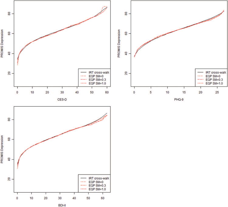
IRT cross-walk function (based on fixed-parameter calibration) and equipercentile functions with different levels of smoothing. PROMIS Depression = Depression subscale of the Patient-Reported Outcomes Measurement Information System; IRT = item response theory; EQP = equipercentile; SM = postsmoothing.

To facilitate the comparison of our linking methods, we computed the correlation, mean difference, and standard deviation of difference scores for the linked T score and the actual PROMIS T score for each method we employed (see Table 4). The method labeled “IRT pattern scoring” refers to IRT scoring based on item parameter estimates and the pattern of responses to those items. We used the conventional Bayes, or expected a posteriori (EAP), estimate (Bock & Mislevy, 1982). The alternative, IRT summed or “cross-walk” scoring, also uses IRT and EAP estimation. In this approach, however, the multiple response patterns that can result in the same summed score are assigned to the same scaled score (Lord & Wingersky, 1984). This calculation is also used to construct the cross-walk table. Table 4 shows that IRT pattern scoring produced the best results for each linking pair; that is, the correlation between actual and linked PROMIS T scores was highest and the standard deviation of differences was lowest (mean differences are misleading because of negative and positive differences). Nevertheless, the differences across methods were small and IRT cross-walk scoring (the basis for the Appendix) was as good as or better than equipercentile linking.

Table 4.

Correlations, Mean Differences, and Standard Deviations of Actual Versus Linked PROMIS Depression T Scores

Linking method/instrument	Correlation	Mean difference	SD of differences
CES-D
IRT pattern scoring	.84	0.31	5.46
IRT cross-walk scoring	.82	0.09	5.78
EQP, SM = 0.0	.81	0.03	5.93
EQP, SM = 0.3	.80	0.30	6.20
EQP, SM = 1.0	.79	0.42	6.46
PHQ-9
IRT pattern scoring	.83	0.36	6.34
IRT cross-walk scoring	.81	0.43	6.73
EQP, SM = 0.0	.80	0.18	6.88
EQP, SM = 0.3	.80	0.06	6.80
EQP, SM = 1.0	.80	0.08	6.82
BDI-II
IRT pattern scoring	.87	0.21	5.87
IRT cross-walk scoring	.86	0.21	6.01
EQP, SM = 0.0	.86	0.14	6.00
EQP, SM = 0.3	.86	0.18	6.00
EQP, SM = 1.0	.86	0.16	6.02

Note. PROMIS = Patient-Reported Outcomes Measurement Information System; IRT = item response theory; CES-D = Center for Epidemiologic Studies Depression Scale; PHQ-9 = 9-item Patient Health Questionnaire; BDI-II = Beck Depression Inventory–II; EQP = equipercentile; SM postsmoothing.

Results of the resampling technique with small subsets (ns = 25, 50, and 75) were consistent for all measures and across all methods. As sample size increased from 25 to 75, the empirical standard error decreased. At n = 75, IRT pattern scoring produced the smallest standard errors: 0.60 (CES-D), 0.69 (PHQ-9), and 0.65 (BDI-II), followed by IRT cross-walk scoring: 0.63 (CES-D), 0.74 (PHQ-9), and 0.67 (BDI-II). In each case, the IRT cross-walk scoring was as good as or better than equipercentile methods. These standard errors can generate confidence intervals around linking results. For example, with a sample of 75 CES-D scores, if one uses the PROsetta Stone table to estimate PROMIS scores, one has 95% confidence that the difference between the mean of this linked PROMIS score and the mean of the PROMIS Depression T score is within ±1.23 T score units (i.e., 1.96 × the 0.63 standard error for CES-D).

Figure 2 shows the test information function (on the PROMIS T score metric) of each instrument and for the combined set of four scales considered as a whole. Among legacy scales, the BDI-II provides the most information (least error) when estimating PROMIS T scores, while the PHQ-9 provides the least information (most error). The accuracy of an average PROMIS score estimated from a sample of legacy scores increases with increasing sample size, as demonstrated in the resampling procedure above.

Figure 2.

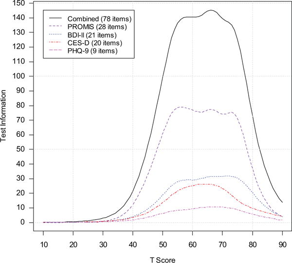
Test information function of each instrument (after linking) and for the combined set of four instruments considered as a whole. PROMIS = Depression subscale of the Patient-Reported Outcomes Measurement Information System; BDI-II = Beck Depression Inventory–II; CES-D = Center for Epidemiologic Studies Depression Scale; PHQ-9 = 9-item Patient Health Questionnaire.

Using the item parameter estimates derived from the fixed-parameter calibration (see Table 3), we constructed a cross-walk table by applying expected a posteriori (EAP) summed scoring (Lord & Wingersky, 1984). The tables for the CES-D, PHQ-9, and BDI-II in the Appendix can be used to map simple raw summed scores from each legacy instrument to T score values on the PROMIS Depression metric. Each raw summed score and corresponding PROMIS T score is presented with the standard error associated with the scaled score. Researchers interested in creating additional cross-walks for various short-forms of the legacy instruments can use subsets of the linked item parameters reported in Table 3, a practice supported by the IRT parameter invariance assumption. In place of the cross-walk table, researchers may wish to score their CES-D, PHQ-9, and BDI-II data on the PROMIS metric, using the parameters in Table 3. Such IRT-pattern scoring is more accurate and follows the standard PROMIS scoring procedure (Cella, Gershon, Bass, & Rothrock, 2013; Gershon, Ro-throck, Hanrahan, Bass, & Cella, 2010).

Figure 3 displays the linking functions for the CES-D, PHQ-9, and BDI-II that map their raw summed scores (the vertical axis) to the PROMIS Depression metric (the horizontal axis). Traditional cutoff scores for the legacy measures are indicated on their respective functions and projected onto the PROMIS metric. Some of the thresholds for possible or moderate depression on the CES-D and BDI-II differ from one another. In fact, the threshold for moderate depression according to the CES-D (about 0.5 SD above the PROMIS population mean) was equivalent to the threshold for mild depression by the BDI-II. However, the thresholds for moderate depression for the BDI-II and PHQ-9 were very similar to each other (about 1 SD above the PROMIS population mean). This is validating the tentative threshold PROMIS has set on the De pression measure of 60, or 1 SD above the population mean (Cella et al., 2008).

Figure 3.

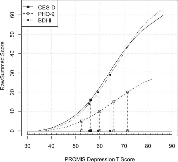
Comparison of clinical cutoff scores on the PROMIS Depression metric. CES-D: 16 or higher for positive clinical depression. PHQ-9: 5–9 (mild), 10–14 (moderate), 15–19 (moderately severe), 20 or higher (Severe). BDI-II: 0–13 (minimal), 14–19 (mild), 20–28 (moderate), 29 or higher (severe). CES-D = Center for Epidemiologic Studies Depression Scale; PHQ-9 = 9-item Patient Health Questionnaire; BDI-II = Beck Depression Inventory–II; PROMIS Depression = Depression subscale of the Patient-Reported Outcomes Measurement Information System.

Discussion

This is the first article that links PROMIS to multiple measures of the same concept, depression, using a methodology that draws from instrument linking in educational testing. Practical products of this effort are the three cross-walk tables (see the Appendix) and a large item bank of IRT-based item parameters anchored on the PROMIS T score metric (see Table 3). Now researchers and clinicians have several options for linking scores on existing depression measures to the PROMIS metric. In this study, IRT methods produced better linking results than did equipercentile linking, but all methods we used produced highly comparable results. The sequential steps of our methods provide a template for future single-group design linking of health outcome domain instruments.

The work reported here has several notable strengths. First, it followed a single-group design, which is optimal for robust linking (Dorans, 2007). Second, we employed multiple linking methods so that we could empirically determine which method minimized differences between observed and linked scores. Third, following Thissen et al. (2011) we calculated the standardized RMSD (Dorans & Holland, 2000) to evaluate subpopulation invariance. This rigorous method is rarely applied in the health outcome literature. Finally, our calibrations were not determined by the current sample but were anchored on the PROMIS calibrations that were derived from the larger standardization sample (Choi et al., 2010; Pilkonis et al., 2011) and centered on the 2000 U.S. Census (Liu et al., 2010).

Utility in Research and Clinical Settings

Our results allow researchers to reconcile single-domain research studies that use different instruments. When outcome studies with different depression outcome instruments show different effects, it is impossible to conclusively determine the cause: Different effects may be attributed to peculiarities in scale content, differences in psychometric properties, or differences in actual treatment effect (e.g., Demyttenaere & de Fruyt, 2003). Discussions on these causes can become speculative and centered on content differences that may be inconsequential. The use of standardized effect sizes does not solve this problem, as they may be sensitive to particular sample characteristics, such as restricted range (Baguley, 2009). Furthermore the aggregation of effect sizes to measure a single construct tends to be an inclusive effort across instruments (as in meta-analyses) typically imposing none of the assumptions enumerated above for our concordance. Thus, IRT-based and equipercentile linking represent a significant advance for comparing effect sizes across measures.

Researchers and clinicians interested in linking any of the three legacy measures to PROMIS Depression have three options. First, they can use the cross-walk chart to substitute each participant’s summed legacy score with the corresponding PROMIS T score. The scores can then be used for descriptive and inferential analyses. Second, researchers can enter the item parameter estimates we obtained for the legacy measures and, using IRT software such as IRTPRO (Cai et al., 2011) or Firestar (Choi, 2009) can obtain scores based on participants’ responses to the items. This approach yields slightly more accurate results than the cross-walk table and also has the advantage of accounting for missing data without imputation. Finally, summary (not individual) sample scores from legacy measures (e.g., as in the case of meta-analyzing published research) can be cross-walked to PROMIS scores and then further aggregated or compared.

Comparison With Other PRO Linking Studies

Several researchers have attempted links between scores on patient-reported outcome instruments. This includes measures of pediatric asthma (Thissen et al., 2011), fatigue (Holzner et al., 2006; Noonan et al., 2012), pain (Chen, Revicki, Lai, Cook, & Amtmann, 2009), functional health status (McHorney & Cohen, 2000), physical functioning (Fisher, Eubanks, & Marier, 1997), and depression (Fischer et al., 2011; Gibbons et al., 2011, 2013; Orlando et al., 2000). Because Gibbons et al. (2011, 2013) published the PHQ-9 parameters on the PROMIS metric, we can compare their results to ours. Given the theoretical population invariance property of IRT parameters, we expected considerable correspondence with our parameters. While the parameters of the first seven items obtained by Gibbons et al. (2013) largely agree with ours, those of the last two items differ substantially. For the items “moves slowly” and “suicidal thinking,” Gibbons et al. (2013) obtained very low discrimination parameters (0.41 and 0.27, respectively). This compares to a range of 1.32 to 3.02 for the remaining items. Our values for those two items were 1.82 and 2.20, respectively.

Criteria for Linking in Health Outcomes

A key criterion for the appropriateness of linking is the correlation coefficient between two instruments. Dorans (2004) suggested that a correlation of .866 is an appropriate lower bound value. This recommendation was made in the context of high-stakes educational testing. Given that the ultimate goal of our project was to compare summed scores of samples (not individuals), we would suggest that linking in health outcomes might follow a slightly relaxed standard. In linking health outcome measures, a correlation of 0.75–0.80 might be an appropriate minimum, especially when a single-sample design is used. Because a single-sample design allows comparison of individuals’ actual scores on a measure to their scores estimated from the linking, the accuracy of the linking can be directly evaluated. Thus, the impact of relaxing prior assumptions can be evaluated in terms of its actual consequences. Ultimately, more important than any correlation criterion is the correspondence between the actual score and the one predicted by the linking.

Despite the strengths of our linking methodology, the resulting scores may have larger error (i.e., measurement error plus linking error) compared to the original instrument scores. Thus, researchers contemplating a switch in instruments during ongoing data collection (e.g., from legacy to PROMIS) should be aware of the associated reduction in reliability. Furthermore, the linking methods used here met the assumptions of construct similarity and unidimensionality. When these assumptions are not met, other methods, such as prediction (Holland, 2007) or calibrated projection (Thissen et al., 2011), may be applied. If neither of the instruments has established calibrations, simultaneous or separate calibration of the measures (instead of fixed calibration) would be more appropriate (e.g., Chen, Revicki, Lai, Cook, & Amtmann, 2009; Orlando et al., 2000). In addition, given the results of our resampling analysis, we note that errors for using the cross-walk tables for samples of 75 or greater will likely be small and acceptable to most users. As the sample size decreases, however, the standard error of differences (linked score minus actual PRO-MIS score) will increase. In the current CES-D study, for example, the standard error for a sample size of 75 was 0.63, but for a single individual it was 5.78. Finally, our linking tables should be used with recognition that concordances between any two instruments (regardless of statistical method) may be sensitive to population differences (Dorans, 2007).

Although we reported on a resampling analysis, it would have been ideal to evaluate the robustness of the linking relationship on a new sample. Such a sample could be used to examine empirically the bias and standard error of the linking results. The small confidence interval we constructed using the resampling technique (e.g., ± 1.23 T score units for CES-D linking, n = 75) may underestimate the error introduced by the linking procedure. Second, although we incorporated widely used depression symptom measures, we did not include any interview-based measures, such as the Hamilton Rating Scale of Depression (HRSD; Hamilton, 1960). Given the heterogeneity of HRSD items and the differences in method of data collection between the HRSD (interview) and PROMIS (self-report), similarly high concordance is less likely but worth evaluating in future research (Demyttenaere & de Fruyt, 2003).

Finally, although the fit statistics of our combined item sets met or exceeded commonly used fit criteria, there is debate over the appropriate cutoff values and the strict adherence to these indices to assess model fit (Lance et al., 2006; Marsh, Hau, & Wen, 2004). Fit indices are sensitive to skewed distributions and number of items (Cook, Kallen, & Amtmann, 2009) as well as methodological artifacts, such as wording (Hopwood & Donnellan, 2010). In the context of IRT analysis of psychological measures, it is important to note that item sets need to be sufficiently unidimensional, ideally considering the preponderance of evidence emerging from a range of statistical indices (Cook et al., 2009; Reise, Cook, & Moore, in press).

In conclusion, this is the first report on health measurement that links more than one legacy scale to the PROMIS metric. We provided several tools for researchers to retrofit scores on three popular depression measures to the PROMIS Depression metric. We also outlined a template for future linking projects involving PRO instruments. Research is under way to complete a large number of additional linking studies to match legacy instruments to many PROMIS instruments and to make the results widely accessible.

Appendix Raw Score to PROMIS Scale Score Conversion Tables

Table A1.

Raw Score to T Score Conversion Table (IRT Fixed-Parameter Calibration Linking) for CES-D to PROMIS Depression

CES-D score	PROMIS Depression T score	SE	CES-D score	PROMIS Depression T score	SE
0	34.5	6.0	30	63.9	2.1
1	38.6	5.1	31	64.4	2.1
2	41.1	4.7	32	64.9	2.1
3	42.9	4.6	33	65.4	2.1
4	44.7	4.1	34	66.0	2.2
5	46.2	3.8	35	66.5	2.2
6	47.5	3.6	36	67.0	2.2
7	48.7	3.4	37	67.6	2.2
8	49.8	3.2	38	68.1	2.2
9	50.8	3.0	39	68.7	2.2
10	51.7	2.9	40	69.2	2.3
11	52.6	2.8	41	69.8	2.3
12	53.4	2.7	42	70.4	2.3
13	54.1	2.6	43	71.0	2.4
14	54.8	2.5	44	71.7	2.4
15	55.5	2.4	45	72.3	2.5
16	56.2	2.4	46	73.0	2.5
17	56.8	2.3	47	73.7	2.6
18	57.4	2.3	48	74.4	2.7
19	58.0	2.3	49	75.2	2.7
20	58.6	2.3	50	76.0	2.8
21	59.1	2.2	51	76.8	2.9
22	59.7	2.2	52	77.7	3.0
23	60.2	2.2	53	78.7	3.1
24	60.8	2.2	54	79.7	3.2
25	61.3	2.2	55	80.8	3.2
26	61.8	2.2	56	82.0	3.2
27	62.3	2.1	57	83.1	3.2
28	62.9	2.1	58	84.3	3.1
29	63.4	2.1	59	85.4	2.8
			60	86.4	2.5

Note. IRT = item response theory; CES-D = Center for Epidemiologic Studies Depression Scale; PROMIS Depression = Depression subscale of the Patient-Reported Outcomes Measurement Information System.

Table A2.

Raw Score to T Score Conversion Table (IRT Fixed-Parameter Calibration Linking) for PHQ-9 to PROMIS Depression

PHQ-9 score	PROMIS Depression T score	SE	PHQ-9 score	PROMIS Depression T score	SE
0	37.4	6.4	14	64.7	3.2
1	42.7	5.3	15	65.8	3.2
2	45.9	4.8	16	66.9	3.2
3	48.3	4.7	17	68.0	3.1
4	50.5	4.3	18	69.2	3.2
5	52.5	4.0	19	70.3	3.2
6	54.2	3.8	20	71.5	3.2
7	55.8	3.7	21	72.7	3.3
8	57.2	3.6	22	74.0	3.4
9	58.6	3.5	23	75.3	3.5
10	59.9	3.4	24	76.7	3.6
11	61.1	3.3	25	78.3	3.7
12	62.3	3.3	26	80.0	3.8
13	63.5	3.2	27	82.3	3.8

Note. IRT = item response theory; PHQ-9 = 9-item Patient Health Questionnaire; PROMIS Depression = Depression subscale of the Patient-Reported Outcomes Measurement Information System.

Table A3.

Raw Score to T Score Conversion Table (IRT Fixed-Parameter Calibration Linking) for BDI-II to PROMIS Depression

BDI-II score	PROMIS Depression T score	SE	BDI-II score	PROMIS Depression T score	SE
0	34.9	5.8	32	65.8	1.9
1	39.4	4.6	33	66.4	1.9
2	42.3	4.0	34	66.9	1.9
3	44.4	3.6	35	67.4	1.8
4	46.2	3.2	36	67.9	1.8
5	47.6	2.9	37	68.4	1.8
6	48.9	2.7	38	68.9	1.8
7	50.0	2.5	39	69.4	1.8
8	51.0	2.4	40	69.9	1.8
9	51.9	2.3	41	70.4	1.8
10	52.7	2.2	42	70.9	1.8
11	53.5	2.1	43	71.4	1.8
12	54.2	2.1	44	71.9	1.8
13	54.9	2.0	45	72.4	1.9
14	55.6	2.0	46	72.9	1.9
15	56.3	2.0	47	73.5	1.9
16	56.9	2.0	48	74.0	1.9
17	57.5	2.0	49	74.6	1.9
18	58.2	2.0	50	75.2	1.9
19	58.8	1.9	51	75.7	2.0
20	59.3	1.9	52	76.4	2.0
21	59.9	1.9	53	77.0	2.0
22	60.5	1.9	54	77.7	2.1
23	61.1	1.9	55	78.4	2.2
24	61.6	1.9	56	79.1	2.2
25	62.2	1.9	57	79.9	2.3
26	62.7	1.9	58	80.8	2.4
27	63.2	1.9	59	81.8	2.5
28	63.8	1.9	60	82.9	2.6
29	64.3	1.9	61	84.0	2.6
30	64.8	1.9	62	85.1	2.6
31	65.3	1.9	63	86.3	2.4

Note. IRT = item response theory; BDI-II = Beck Depression Inventory–II; PROMIS Depression = Depression subscale of the Patient-Reported Outcomes Measurement Information System.

References

- Albano T. equate: Statistical methods for test score equating (R Package Version 1.1–4 [Computer software] 2011 Retrieved from http://cran.r-project.org/web/packages/equate/vignettes/equatevignette.pdf.
- American Psychiatric Association. Diagnostic and statistical manual of mental disorders. 4th. Washington, DC: Author; 1994. [Google Scholar]
- American Psychiatric Association. Diagnostic and statistical manual of mental disorders. 5th. Arlington, VA: American Psychiatric Publishing; 2013. [Google Scholar]
- Baguley T. Standardized or simple effect size: What should be reported? British Journal of Psychology. 2009;100:603–617. doi: 10.1348/000712608X377117. [DOI] [PubMed] [Google Scholar]
- Beck AT. Depression: Causes and treatment. Philadelphia, PA: University of Pennsylvania Press; 1967. [Google Scholar]
- Beck AT, Rush AJ, Shaw BF, Emery G. Cognitive therapy of depression. New York, NY: Guilford Press; 1979. [Google Scholar]
- Beck AT, Steer RA, Brown GK. Manual for the Beck Depression Inventory-II. San Antonio, TX: Psychological Corporation; 1996. [Google Scholar]
- Bock RD, Mislevy RJ. Adaptive EAP estimation of ability in a microcomputer environment. Applied Psychological Measurement. 1982;6:431–444. doi: 10.1177/014662168200600405. [DOI] [Google Scholar]
- Brennan R. Linking with Equivalent Group or Single Group Design (LEGS; Version 2.0) [Computer software] Iowa City, IA: University of Iowa, Center for Advanced Studies in Measurement and Assessment (CASMA); 2004. [Google Scholar]
- Buysse DJ, Yu L, Moul DE, Germain A, Stover A, Dodds NE, Pilkonis PA. Development and validation of patient-reported outcome measures for sleep disturbance and sleep-related impairments. Sleep. 2010;33:781–792. doi: 10.1093/sleep/33.6.781. [DOI] [PMC free article] [PubMed] [Google Scholar]
- Cai L, Thissen D, du Toit S. IRTPRO 2.01 [Computer software] Lincolnwood, IL: Scientific Software International; 2011. [Google Scholar]
- Cella D, Choi S, Rosenbloom S, Surges Tatum D, Garcia S, Lai JS, Gershon R. A novel IRT-based case-ranking approach to derive expert standards for symptom severity. Quality of Life Research. 2008;17(Suppl. 1):A-32. [Google Scholar]
- Cella D, Gershon R, Bass M, Rothrock N. PROMIS Depression Scoring Manual. 2013 Retrieved from http://www.assessmentcenter.net/documents/PROMIS%20Depression%20Scoring%20Manual.pdf.
- Cella D, Riley W, Stone A, Rothrock N, Reeve B, Yount S, Hays R. The Patient-Reported Outcomes Measurement Information System (PROMIS) developed and tested its first wave of adult self-reported health outcome item banks: 2005–2008. Journal of Clinical Epidemiology. 2010;63:1179–1194. doi: 10.1016/j.jclinepi.2010.04.011. [DOI] [PMC free article] [PubMed] [Google Scholar]
- Cella D, Yount S, Rothrock N, Gershon R, Cook K, Reeve B, Rose M. The Patient-Reported Outcomes Measurement Information System (PROMIS): Progress of an NIH roadmap cooperative group during its first two years. Medical Care. 2007;45:S3–S11. doi: 10.1097/01.mlr.0000258615.42478.55. [DOI] [PMC free article] [PubMed] [Google Scholar]
- Chen WH, Revicki DA, Lai J, Cook KF, Amtmann D. Linking pain items from two studies onto a common scale using item response theory. Journal of Pain and Symptom Management. 2009;38:615–628. doi: 10.1016/j.jpainsymman.2008.11.016. [DOI] [PMC free article] [PubMed] [Google Scholar]
- Chen WH, Thissen D. Local dependence indexes for item pairs using item response theory. Journal of Educational and Behavioral Statistics. 1997;22:265–289. doi: 10.3102/10769986022003265. [DOI] [Google Scholar]
- Choi SW. Firestar: Computerized adaptive testing simulation program for polytomous IRT models. Applied Psychological Measurement. 2009;33:644–645. doi: 10.1177/0146621608329892. [DOI] [Google Scholar]
- Choi SW, Reise SP, Pilkonis PA, Hays RD, Cella D. Efficiency of static and computer adaptive short forms compared to full length measures of depressive symptoms. Quality of Life Research. 2010;19:125–136. doi: 10.1007/s11136-009-9560-5. [DOI] [PMC free article] [PubMed] [Google Scholar]
- Cook KF, Kallen MA, Amtmann D. Having a fit: Impact of number of items and distribution of data on traditional criteria for assessing IRT’s unidimensionality assumption. Quality of Life Research. 2009;18:447–460. doi: 10.1007/s11136-009-9464-4. [DOI] [PMC free article] [PubMed] [Google Scholar]
- Demyttenaere K, De Fruyt J. Getting what you ask for: On the selectivity of depression rating scales. Psychotherapy and Psychosomatics. 2003;72:61–70. doi: 10.1159/000068690. [DOI] [PubMed] [Google Scholar]
- DeWalt DA, Rothrock N, Yount S, Stone AA. Evaluation of item candidates: The PROMIS qualitative item review. Medical Care. 2007;45(Suppl. 1):S12–S21. doi: 10.1097/01.mlr.0000254567.79743.e2. [DOI] [PMC free article] [PubMed] [Google Scholar]
- Dorans NJ. Equating, concordance, and expectation. Applied Psychological Measurement. 2004;28:227–246. doi: 10.1177/0146621604265031. [DOI] [Google Scholar]
- Dorans NJ. Linking scores from multiple health outcome instruments. Quality of Life Research. 2007;16(1 Suppl):85–94. doi: 10.1007/s11136-006-9155-3. [DOI] [PubMed] [Google Scholar]
- Dorans NJ, Holland PW. Population invariance and the equatability of tests: Basic theory and the linear case. Journal of Educational Measurement. 2000;37:281–306. doi: 10.1111/j.1745-3984.2000.tb01088.x. [DOI] [Google Scholar]
- Dum M, Pickren J, Sobell LC, Sobell MB. Comparing the BDI-II and the PHQ-9 with outpatient substance abusers. Addictive Behaviors. 2008;33:381–387. doi: 10.1016/j.addbeh.2007.09.017. [DOI] [PubMed] [Google Scholar]
- Fischer HF, Tritt K, Klapp BF, Fliege H. How to compare scores from different depression scales: Equating the Patient Health Questionnaire (PHQ) and the ICD-10-Symptom Rating (ISR) using item response theory. International Journal of Methods in Psychiatric Research. 2011;20:203–214. doi: 10.1002/mpr.350. [DOI] [PMC free article] [PubMed] [Google Scholar]
- Fisher WP, Jr, Eubanks RL, Marier RL. Equating the MOS SF36 and the LSU HSI physical functioning scales. Journal of Outcome Measurement. 1997;1:329–362. [PubMed] [Google Scholar]
- Fries JF, Cella D, Rose M, Krishnan E, Bruce B. Progress in assessing physical function in arthritis: PROMIS short forms and computerized adaptive testing. Journal of Rheumatology. 2009;36:2061–2066. doi: 10.3899/jrheum.090358. [DOI] [PubMed] [Google Scholar]
- Gershon RC, Rothrock N, Hanrahan R, Bass M, Cella D. The use of PROMIS and assessment center to deliver patient-reported outcome measures in clinical research. Journal of Applied Measurement. 2010;11:304–314. [PMC free article] [PubMed] [Google Scholar]
- Gershon RC, Wagster MV, Hendrie HC, Fox NA, Cook KF, Nowinski CJ. NIH Toolbox for assessment of neurological and behavioral function. Neurology. 2013;80(11 Suppl. 3):S2–S6. doi: 10.1212/WNL.0b013e3182872e5f. [DOI] [PMC free article] [PubMed] [Google Scholar]
- Gibbons LE, Feldman BJ, Crane HM, Mugavero M, Willig JH, Patrick D, Crane PK. Migrating from a legacy fixed-format measure to CAT administration: Calibrating the PHQ-9 to the PROMIS depression measures. Quality of Life Research. 2011;20:1349–1357. doi: 10.1007/s11136-011-9882-y. [DOI] [PMC free article] [PubMed] [Google Scholar]
- Gibbons LE, Feldman BJ, Crane HM, Mugavero M, Willig JH, Patrick D, Crane PK. Erratum to: Migrating from a legacy fixed-format measure to CAT administration: Calibrating the PHQ-9 to the PROMIS depression measures. Quality of Life Research. 2013;22:459–460. doi: 10.1007/s11136-012-0313-5. [DOI] [PMC free article] [PubMed] [Google Scholar]
- Haebara T. Equating logistic ability scales by a weighted least squares method. Japanese Psychological Research. 1980;22:144–149. [Google Scholar]
- Hamilton M. A rating scale for depression. Journal of Neurology, Neurosurgery, & Psychiatry. 1960;23:56–62. doi: 10.1136/jnnp.23.1.56. [DOI] [PMC free article] [PubMed] [Google Scholar]
- Hepner KA, Hunter SB, Edelen MO, Zhou AJ, Watkins K. A comparison of two depressive symptomatology measures in residential substance abuse treatment clients. Journal of Substance Abuse Treatment. 2009;37:318–325. doi: 10.1016/j.jsat.2009.03.005. [DOI] [PMC free article] [PubMed] [Google Scholar]
- Holland PW. A framework and history for score linking. In: Dorans NJ, Pommerich M, Holland PW, editors. Linking and aligning scores and scales. New York, NY: Springer; 2007. pp. 5–30. [Google Scholar]
- Holzner B, Bode RK, Hahn EA, Cella D, Kopp M, Sperner-Unterweger B, Kemmler G. Equating EORTC QLQ-C30 and FACT-G scores and its use in oncological research. European Journal of Cancer. 2006;42:3169–3177. doi: 10.1016/j.ejca.2006.08.016. [DOI] [PubMed] [Google Scholar]
- Hopwood CJ, Donnellan MB. How should the internal structure of personality inventories be evaluated? Personality and Social Psychology Review. 2010;14:332–346. doi: 10.1177/1088868310361240. [DOI] [PubMed] [Google Scholar]
- Kelly MAR, Morse JQ, Stover A, Hofkens T, Huisman E, Shulman S, Pilkonis PA. Describing depression: Congruence between patient experiences and clinical assessments. British Journal of Clinical Psychology. 2011;50:46–66. doi: 10.1348/014466510X493926. [DOI] [PMC free article] [PubMed] [Google Scholar]
- Kolen MJ, Brennan RL. Test equating, scaling, and linking: Methods and practices. 2004 doi: 10.1007/978-1-4757-4310-4. [DOI] [Google Scholar]
- Kroenke K, Spitzer RL, Williams JBW. The PHQ-9 validity of a brief depression severity measure. Journal of General Internal Medicine. 2001;16:606–613. doi: 10.1046/j.1525-1497.2001.016009606.x. [DOI] [PMC free article] [PubMed] [Google Scholar]
- Kuhl EA, Kupfer DJ, Regier DA. Patient-centered revisions to the DSM-5. Virtual Mentor. 2011;13:873–879. doi: 10.1001/virtualmentor.2011.13.12.stas1-1112. [DOI] [PubMed] [Google Scholar]
- Kung S, Alarcon RD, Williams MD, Poppe KA, Moore MJ, Frye MA. Comparing the Beck Depression Inventory-II (BDI-II) and Patient Health Questionnaire (PHQ-9) depression measures in an integrated mood disorders practice. Journal of Affective Disorders. 2012;145:341–343. doi: 10.1016/j.jad.2012.08.017. [DOI] [PubMed] [Google Scholar]
- Lance CE, Butts MM, Michels LC. The sources of four commonly reported cutoff criteria: What did they really say? Organizational Research Methods. 2006;9:202–220. doi: 10.1177/1094428105284919. [DOI] [Google Scholar]
- Liu H, Cella D, Gershon R, Shen J, Morales LS, Riley W, Hays RD. Representativeness of the PROMIS Internet panel. Journal of Clinical Epidemiology. 2010;63:1169–1178. doi: 10.1016/j.jclinepi.2009.11.021. [DOI] [PMC free article] [PubMed] [Google Scholar]
- Liu Y, Thissen D. Identifying local dependence with a score test statistic based on the bifactor logistic model. Applied Psychological Measurement. 2012;36:670–688. doi: 10.1177/0146621612458174. [DOI] [Google Scholar]
- Lord FM. The standard error of equipercentile equating. Journal of Educational and Behavioral Statistics. 1982;7:165–174. doi: 10.3102/10769986007003165. [DOI] [Google Scholar]
- Lord FM, Wingersky MS. Comparison of IRT true-score and equipercentile observed-score “equatings”. Applied Psychological Measurement. 1984;8:453–461. doi: 10.1177/014662168400800409. [DOI] [Google Scholar]
- Löwe B, Kroenke K, Gräfe K. Detecting and monitoring depression with a two-item questionnaire (PHQ-2) Journal of Psychosomatic Research. 2005;58(2):163–171. doi: 10.1016/j.jpsychores.2004.09.006. [DOI] [PubMed] [Google Scholar]
- Marsh HW, Hau KT, Wen Z. In search of golden rules: Comment on hypothesis-testing approaches to setting cutoff values for fit indices and dangers in overgeneralizing Hu and Bentler’s (1999) findings. Structural Equation Modeling. 2004;11:320–341. doi: 10.1207/s15328007sem1103_2. [DOI] [Google Scholar]
- McDonald RP. Test theory: A unified treatment. Mahwah, NJ: Erlbaum; 1999. [Google Scholar]
- McHorney CA, Cohen AS. Equating health status measures with item response theory: Illustrations with functional status items. Medical Care. 2000;38(9 Suppl):II-43–II-59. doi: 10.1097/00005650-200009002-00008. [DOI] [PubMed] [Google Scholar]
- Milette K, Hudson M, Baron M, Thombs BD. Comparison of the PHQ-9 and CES-D depression scales in systemic sclerosis: Internal consistency reliability, convergent validity and clinical correlates. Rheumatology. 2010;49:789–796. doi: 10.1093/rheumatology/kep443. [DOI] [PubMed] [Google Scholar]
- Muthén LK, Muthén BO. Mplus [Computer software] Los Angeles, CA: Muthén & Muthén; 2006. [Google Scholar]
- Myers JK, Weissman MM. Use of a self-report symptom scale to detect depression in a community sample. American Journal of Psychiatry. 1980;137:1081–1084. doi: 10.1176/ajp.137.9.1081. [DOI] [PubMed] [Google Scholar]
- Naughton MJ, Wiklund II. A critical review of dimension-specific measures of health-related quality of life in cross-cultural research. Quality of Life Research. 1993;2:397–432. doi: 10.1007/BF00422216. [DOI] [PubMed] [Google Scholar]
- Noonan VK, Cook KF, Bamer AM, Choi SW, Kim J, Amtmann D. Measuring fatigue in persons with multiple sclerosis: Creating a crosswalk between the Modified Fatigue Impact Scale and the PROMIS Fatigue Short Form. Quality of Life Research. 2012;21:1123–1133. doi: 10.1007/s11136-011-0040-3. [DOI] [PubMed] [Google Scholar]
- Orlando M, Sherbourne CD, Thissen D. Summed-score linking using item response theory: Application to depression measurement. Psychological Assessment. 2000;12:354–359. doi: 10.1037/1040-3590.12.3.354. [DOI] [PubMed] [Google Scholar]
- Pilkonis PA, Choi SW, Reise SP, Stover AM, Riley WT, Cella D. Item banks for measuring emotional distress from the Patient-Reported Outcomes Measurement Information System (PROMIS®): Depression, anxiety, and anger. Assessment. 2011;18:263–283. doi: 10.1177/1073191111411667. [DOI] [PMC free article] [PubMed] [Google Scholar]
- Pilkonis PA, Choi SW, Salsman JM, Butt Z, Moore TL, Lawrence SM, Cella D. Assessment of self-reported negative affect in the NIH Toolbox. Psychiatry Research. 2013;206:88–97. doi: 10.1016/j.psychres.2012.09.034. [DOI] [PMC free article] [PubMed] [Google Scholar]
- Quilty LC, Bagby R. The assessment of depressive severity: A review. Directions in Psychiatry. 2008;28:135–146. [Google Scholar]
- Radloff LS. The CES-D Scale: A self-report depression scale for research in the general population. Applied Psychological Measurement. 1977;1:385–401. doi: 10.1177/014662167700100306. [DOI] [Google Scholar]
- Radloff LS, Locke BZ. The Community Mental Health Assessment Survey and the CES-D Scale. In: Weissman MM, Myers JK, Ross CE, editors. Community surveys of psychiatric disorders. New Brunswick, NJ: Rutgers University Press; 1986. pp. 177–189. [Google Scholar]
- R Core Development Team. R: A language and environment for statistical computing [Computer software] 2011 Retrieved from http://www.r-project.org/
- Reeve BB, Hays RD, Bjorner JB, Cook KF, Crane PK, Teresi JA, Cella D. Psychometric evaluation and calibration of health-related quality of life item banks: Plans for the Patient-Reported Outcomes Measurement Information System (PROMIS) Medical Care. 2007;45(Suppl. 1):S22–S31. doi: 10.1097/01.mlr.0000250483.85507.04. [DOI] [PubMed] [Google Scholar]
- Reinsch CH. Smoothing by spline functions. Numerische Mathematik. 1967;10:177–183. doi: 10.1007/BF02162161. [DOI] [Google Scholar]
- Reise SP, Cook KF, Moore TM. Evaluating the impact of multidimensionality on unidimensional item response theory model parameters. In: Reise SP, Revicki DA, editors. Multivariate Applications Series: Vol ?? Handbook of item response theory modeling: Applications to typical performance assessment. New York, NY: Routledge/Taylor & Francis Group; pp. XXX–XXX. (in press) [Google Scholar]
- Reise SP, Scheines R, Widaman KF, Haviland MG. Multidimensionality and structural coefficient bias in structural equation modeling: A bifactor perspective. Educational and Psychological Measurement. 2013;73:5–26. doi: 10.1177/0013164412449831. [DOI] [Google Scholar]
- Revelle W. psych: Procedures for personality and psychological research (R Package Version 1.2.8) [Computer software] 2013 Retrieved from http://cran.r-project.org/web/packages/psych/index.html.
- Revicki DA, Chen W, Harnam N, Cook KF, Amtmann D, Callahan LF, Keefe FJ. Development and psychometric analysis of the PROMIS pain behavior item bank. Pain. 2009;146:158–169. doi: 10.1016/j.pain.2009.07.029. [DOI] [PMC free article] [PubMed] [Google Scholar]
- Schmid JJ, Leiman JM. The development of hierarchical factor solutions. Psychometrika. 1957;22:53–61. doi: 10.1007/BF02289209. [DOI] [Google Scholar]
- Shean G, Baldwin G. Sensitivity and specificity of depression questionnaires in a college-age sample. Journal of Genetic Psychology. 2008;169:281–292. doi: 10.3200/GNTP.169.3.281-292. [DOI] [PubMed] [Google Scholar]
- Stocking ML, Lord FM. Developing a common metric in item response theory. Applied Psychological Measurement. 1983;7:201–210. doi: 10.1177/014662168300700208. [DOI] [Google Scholar]
- Thissen D, Chen WH, Bock RD. Multilog 7.03 [Computer software] Lincolnwood, IL: Scientific Software International; 2003. [Google Scholar]
- Thissen D, Varni JW, Stucky BD, Liu Y, Irwin DE, DeWalt DA. Using the PEDSQL™ 3.0 asthma module to obtain scores comparable with those of the PROMIS Pediatric Asthma Impact Scale (PAIS) Quality of Life Research. 2011;20:1497–1505. doi: 10.1007/s11136-011-9874-y. [DOI] [PMC free article] [PubMed] [Google Scholar]
- Titov N, Dear BF, McMillan D, Anderson T, Zou J, Sunderland M. Psychometric comparison of the PHQ-9 and BDI-II for measuring response during treatment of depression. Cognitive Behaviour Therapy. 2011;40:126–136. doi: 10.1080/16506073.2010.550059. [DOI] [PubMed] [Google Scholar]
- Tritt K, Heymann F, Zaudig M, Zacharias I, Söllner W, Loew TH. Entwicklung des Fragebogens ‘ICD-10-Symptomrating’ (ISR) [Development of the questionnaire ‘ICD-10-Symptom Rating’ (ISR)] Zeitschrift für Psychosomatische Medizin und Psychotherapie. 2008;54:425–434. doi: 10.13109/zptm.2008.54.4.409. [DOI] [PubMed] [Google Scholar]
- Weeks JP. Plink: An R package for linking mixed-format tests using IRT-based methods. Journal of Statistical Software. 2010;35:1–33. [Google Scholar]
- Weissman MM, Sholomskas D, Pottenger M, Prusoff BA, Locke BZ. Assessing depressive symptoms in five psychiatric populations: A validation study. American Journal of Epidemiology. 1977;106:203–214. doi: 10.1093/oxfordjournals.aje.a112455. [DOI] [PubMed] [Google Scholar]
- World Health Organization. Constitution of the World Health Organization: Basic documents. 46th. Geneva, Switzerland: Author; 2007. [Google Scholar]
- Zimmerman M, Coryell W. Screening for major depressive disorder in the community: A comparison of measures. Psychological Assessment. 1994;6:71–74. doi: 10.1037/1040-3590.6.1.71. [DOI] [Google Scholar]
- Zinbarg RE, Revelle W, Yovel I, Li W. Cronbach’s α, Revelle’s β, and Mcdonald’s ωh, their relations with each other and two alternative conceptualizations of reliability. Psychometrika. 2005;70:123–133. doi: 10.1007/s11336-003-0974-7. [DOI] [Google Scholar]