Multi-Parameter Ensemble Learning for Automated Vertebral Body Segmentation in Heterogeneously Acquired Clinical MR Images

Abstract

The development of quantitative imaging biomarkers in medicine requires automatic delineation of relevant anatomical structures using available imaging data. However, this task is complicated in clinical medicine due to the variation in scanning parameters and protocols, even within a single medical center. Existing literature on automatic image segmentation using MR data is based on the analysis of highly homogenous images obtained using a fixed set of pulse sequence parameters (TR/TE). Unfortunately, algorithms that operate on fixed scanning parameters do not avail themselves to real-world daily clinical use due to the existing variation in scanning parameters and protocols. Thus, it is necessary to develop algorithmic techniques that can address the challenge of MR image segmentation using real clinical data. Toward this goal, we developed a multi-parametric ensemble learning technique to automatically detect and segment lumbar vertebral bodies using MR images of the spine. We use spine imaging data to illustrate our techniques since low back pain is an extremely common condition and a typical spine clinic evaluates patients that have been referred with a wide range of scanning parameters. This method was designed with special emphasis on robustness so that it can perform well despite the inherent variation in scanning protocols. Specifically, we show how a single multi-parameter ensemble model trained with manually labeled T2 scans can autonomously segment vertebral bodies on scans with echo times varying between 24 and 147 ms and relaxation times varying between 1500 and 7810 ms. Furthermore, even though the model was trained using T2-MR imaging data, it can accurately segment vertebral bodies on T1-MR and CT, further demonstrating the robustness and versatility of our methodology. We believe that robust segmentation techniques, such as the one presented here, are necessary for translating computer assisted diagnosis into everyday clinical practice.

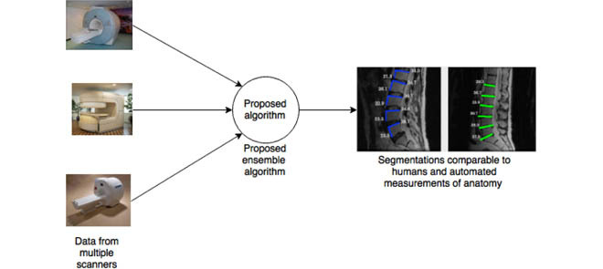
Our proposed algorithm can accurately segment spinal vertebrae even when the images are acquired using several different scanners at several different clinical imaging centers.

I. Introduction

The ability to autonomously segment relevant anatomical structures could substantially augment and improve medical diagnosis. This improvement will be realized through quantitative analysis of pathological changes, versus the current qualitative interpretation, as well as through automated detection of subtle anatomical changes/defects. Yet achieving this vision without lengthening the clinical workflow requires automatic delineation of anatomical structures on medical images (medical image segmentation). While a large body of literature has been dedicated to medical image segmentation, the development of medical image segmentation techniques that are robust to variation in scanning protocol and presence of pathology presents a substantial challenge to existing algorithms. Furthermore, we believe it is an area of research that is not sufficiently addressed in the current literature. This is especially true of spineMRimaging, wherein it is an especially pressing clinical problem due to the high prevalence of low back pain in the global population and a lack of clear understanding of its etiology. This lack of understanding can be partly ascribed to a lack of quantitative anatomical measures when evaluating patients with low back pain. Availability of image-based biomarkers can address this challenge. Since the majority of current diagnostic paradigms for low back pain inevitably rely on magnetic resonance imaging (MRI), this is an important clinical need for MRI based biomarker development. While gross pathological defects can be easily noted visually, subtle degenerative changes in a given patient’s anatomy are far more difficult to assess in routine radiologic screening. Furthermore, current diagnostic technologies do not offer a reliable methodology to quantify an anatomic aberration/pathology or provide a means for quantitative comparison with a healthy control. Manual or semi-automated delineation of vertebral bodies and related structures is not practical in a clinical environment due to time constraints, which renders quantitative assessment based on current technology infeasible. Thus, there is a need to develop fully automated techniques for delineating spinal vertebrae, as well as other anatomical structures, on MR images.

A large proportion of efforts addressing this need have centered around the use of CT data, while the use of MR has been relatively limited. Often, existing methodologies using MR utilize a single dataset acquired in a research setting with a single set of parameters. We will reviewsome of the existing literature and elucidate key differentiators. Most literature on segmentation of lumbar vertebral body segmentation focuses on the use of CT images. This is perhaps understandable given the relative contrast of vertebral bodies (bone) on CT and the fact that CT is the defacto modality in trauma and analysis/detection of fractures. Notable work in segmentation of spinal CT includes [3], [12], [17], and [29]. However, CT imaging is of limited utility in the evaluation of patients with low back pain and radiculopathy due to the poor resolution of soft tissue structures (e.g. disks, ligaments). As such, delineation of vertebral bodies serves as a primary step for the segmentation of associated spinal structures. Thus, vertebral body segmentation is the focus of the current work.

A review of the literature reveals that the large majority of vertebral segmentation methods using MR have focused on semi-automatic segmentation, wherein a clinician supplies seed points defining regions inside and outside the vertebral body. These include graph cut based methods [3], [9], [20], methods based on watershed segmentation [4], [5], [30], and methods based on level sets [17]. Fully automatic localization of vertebral discs on MR has been addressed relatively sparsely. Notable works include the use of Adaboost in combination with a localized model in [29] and the disc localization work presented in [2] and [7]. There are relatively few groups that have addressed fully (with no manual intervention), detection and segmentation of vertebral bodies on MR images. Recent work includes [26] where the authors utilize sparse kernel machines to construct a nonlinear boundary regression model to detect and segment vertebrae. However, the data set employed in this work consists of highly homogeneous image acquisition protocol (TE of 85ms and TR of 4000ms). Peng et al. [19] present a detection and segmentation technique but again validate it on a small uniform data set acquired in a single scanner setting. Neubert et al. [18] use shape models on a data set scanned using a single 3T scanner acquired completely from asymptomatic subjects. Perhaps the closest work to the current manuscript is presented in [14] where a fully automated learning based method is presented using a detector similar to Viola-Jones and a variant of normalized cuts. However, even there the dataset variation is not very high. The work presented in [14] also highlights another key aspect of existing literature, namely, a separate validation step for detection and segmentation. Such an approach is necessary when evaluating segmentation techniques that rely on human based detection (or a different detection algorithm). Since the proposed approach integrates the detection step with the segmentation step and operates without human supervision of any form, we validate the technique by comparing segmentations generated by our technique to those generated by humans.

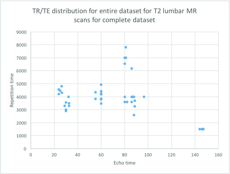
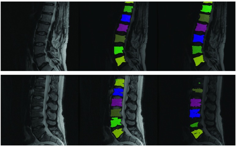
Ultimately, we would like to emphasize that each of these approaches have their respective merits, but they are validated with a very specific dataset obtained under specific pulse sequences and, most often in asymptomatic patients. Real world clinical data is neither obtained from asymptomatic patients nor from a single type of scanner. Thus, translation of the previously described approaches to the clinical setting leads to underwhelming results. It was this need that motivated the development of an ensemble method for the detection and segmentation of vertebral bodies on a wide array of spinal MR images. Our data set was collected as a part of an active, spine clinic that serves as a major tertiary referral center. Since patients were referred to this clinic from the greater Los Angeles area, the accompanying imaging data was acquired at a variety of regional radiology centers. Consequently, there was substantial variation in TR/TE, pixel sizes and image resolutions in our data (see Figure 1). It is important to put this into perspective: one of the more recent works on spine segmentation presented in this journal [26] uses data wherein more than 90% of the images were acquired with a fixed set of pulse sequence parameters. Segmentation of vertebral bodies in the presence of varying acquisition parameters is challenging (see Figure 2). Perhaps this explains why vendors of computer aided diagnostic (CAD) software often bundle their tools for sale with specific scanners rather than standalone software. In practice such an approach severely limits the applicability of CAD by relegating it to a point of scan process rather than a point of utilization process.

FIGURE 1.

Variation in relaxation and echo time in T2-MRIs seen in a routine spine clinic.

FIGURE 2.

Why a majority of segmentation algorithms developed for CAD do not often translate to the clinic: Left column shows two clinical T2 scans. Middle column shows results from our proposed fully automated ensemble technique using several parameter values. Right column shows ITK’s watershed algorithm operating using a fixed set of parameter values initialized to vertebral centers assuming perfect detection of such centers. While the specific set of parameter values chosen works for the image in the top row, it fails for the image in the bottom row. Our technique works for both images.

If CAD techniques are to be clinically useful, it is critical that they be developed in a manner such that they are robust to scanner and sequence variation. Thiswas the driving factor that lead us to develop an ensemble based algorithm for the robust segmentation of lumbar vertebrae. To achieve even modest results in a clinical environment, we had to use a combination of state of the art computer vision and machine learning for performing these segmentations. In the subsequent Methods section, we describe our method along with the motivation and intuition behind each component. Succinctly, our method uses a random forest classifier to identify super-pixels that may be representative of vertebral bodies. While this approach alone is powerful, it often fails in the clinical data sets used in our experiments. The solution to this problem is to vary the parameters used to run the Felzenswalb superpixel algorithm over a large range of values and train a separate random forest to identify vertebral bodies at each parameter setting. The aggregation of vertebral superpixels over all possible parameter values yields a robust segmentation algorithm. Since each classifier trained as a part of our ensemble uses a different parameter setting, we call the overall classifier a multi-parameter ensemble. Empirical evaluation suggests that this approach is extremely robust to variation in the underlying data set. We trained our system on six manually segmented T2-MR images and the trained model could accurately segment T2 as well as T1 MR images obtained using a wide range of acquisition settings. In the following sections we present our method as well as experiments comparing our technique with manual segmentations. A brief discussion on future work concludes the manuscript.

II. Methods

A. Dataset Details

As previously stated majority of the T2-MR dataset (33 lumbar sagittal cases) used for this study was obtained from an active spine clinic. To this we added a set of (15 lumbar sagittal cases T2 and T1) available from the public repository of spine images (http://spineweb.digitalimaginggroup.ca/). Thus, we had 48 sagittal T2-MR scans and 15 T1-MR scans. We used 6 (randomly selected) T2-scans for training the segmentation tool and the rest for validation. The training procedure was computationally expensive. Our present implementation required to 12 to 14 hours to train on our 6-core Mac Pro. Thus, we limited the training set to a maximum of 6 cases for this manuscript. While we expect a larger training set to produce better segmentations, this is currently beyond our computational capacity. To further elucidate the effect of the size of training data, we present results from experiments with training sets smaller in size than 6 cases in the discussion section. The primary focus of this work was to develop a clinically usable technique to segment vertebral bodies on T2-MR despite enormous variation. Thus, majority of validation focused on T2-MR images. Relaxation time (TR) used to acquire images labeled as T2-MRI varied between a maximum of 7810ms and a minimum of 1500ms with a mean of 3798 ms (standard deviation 1575 ms). Excitation time (TE) for these images varied between a minimum of 24ms and a maximum of 147ms with a mean of 77ms (standard deviation of 40.21ms). Apart from the variation in TR and TE, the T2-images also had substantial variation in pixel resolution and as well as acquisition dimensions. Pixel dimensions in the sagittal plane varied between a minimum of mm to a maximum of mm with a mean of mm (with standard deviation 0.21mm). Slice thickness, on the other hand varied between 0.5 mm at minimum to 5.0 mm at a maximum with mean of 3.15mm (and standard deviation of 1.5mm). Image sizes corresponding to the lumbar spine correspondingly varied between pixels to pixels. The dataset had T1-MR images obtained from the publicly available dataset had slice thicknesses varying between 1mm and 5mm with a mean of of 4 mm (with standard deviation of 0.9 mm), and pixel width varying between 0.4mm and 0.7mm with a mean of 0.5 mm (with standard deviation of 0.06 mm). TE was between 14ms and 25ms with mean 18ms (standard deviation 5.6ms) and TR was between 383ms and 3500ms with mean of 1375ms (standard deviation 1255ms). The primary variability present in this dataset comes from the fact that it was sourced from multiple scanners at multiple centers and was acquired using multiple protocols. A secondary source of variability comes from the fact that there is a mix of normal subjects from the publicly available dataset with patients from the Los Angeles clinics.

B. Intuition

The segmentation framework presented is inspired by the ensemble learning principles upon which classic learning algorithms such as the random forest are based. To understand intuitively, how we apply this principle, consider a toy image containing just two vertebral bodies (VBs) denoted as and . Suppose we were to apply a super-pixel algorithm in a classic sense, then it would be unreasonable to expect that superpixels corresponding to each VB pop up. However, if every super-pixel algorithm (and indeed every segmentation algorithm) is ultimately driven by a small set of parameter values. Suppose at parameter setting the algorithm captures accurately but segments poorly. Now, if we change to the algorithm may capture accurately as one of its super-pixels, while improperly segmenting . The only way to get the algorithm to accurately segment both and is to run it at multiple parameter values followed by a classification step that separates super-pixels likely to represent vertebral bodies from those that may not. Thus, in a gestalt sense, the super-pixel algorithms operating at a single parameter setting operate as individual learners. While each individual learner produced imperfect segmentations, a combination of these segmentations can yield a powerful segmentation tool. Next we describe the specific super-pixelization framework we use and how feature extraction is done on the basis of these superpixels.

C. Felzenszwalb Superpixels

Superpixel algorithms divide an image into a set of sub regions such that each sub region is homogeneous according to some criterion. Our technique ultimately relies on the possibility that a vertebral body be captured in a single superpixel by the algorithm. Since super pixel algorithms differ depending on the specific criterion used to assess homogeneity, this can be difficult to achieve in practice. In this work we use the superpixel segmentation algorithm proposed by [10].

1). Motivation

The motivation behind this is that this algorithm generates superpixels by examining evidence for a boundary between two neighboring regions as opposed to raw intensity based pixel grouping produced by algorithms such a SLIC [1]. or local quickshift clustering. Thus, gradual variation in intensity due to the existence of a strong bias field that does not produce explicit edges in the image is likely to be ignored by Felzenswalb superpixels (unlike competing methods like SLIC or quickshift superpixels). This is especially valuable, since strong bias fields designed to attenuate signals in the abdominal regions while amplifying signals on the posterior regions of the body are characteristic of spine MRIs. Such bias fields cannot be corrected by the application of N4 [23] or N3 [21]. The Felzenswalb technique remains robust to the bias field over a wide range of parameters. This is illustrated in 3 where for each parameter setting the Felzenszwalb algorithm picks a few superpixels that correspond to vertebral bodies. This is not true of SLIC which tends to produce superpixels that adhere to vertebral boundaries only at specific parameter settings. Finding the ideal parameter setting for every variant of a spine image immediately makes manual parameter tuning an essential part of the segmentation process with competing techniques. The need for such manual tuning, is exactly what renders a large variety of published segmentation methods impractical for direct use in a typical clinical setting. Figure 3 immediately motivates a multi-parameter learning algorithm. Essentially, if we could train a learning algorithm to identify precisely those superpixels that correspond to vertebral bodies, at given parameter setting, we could create a powerful segmentation method by simply aggregating relevant segments over all parameter values. This is the essence of the proposed procedure.

FIGURE 3.

Felzenszwalb superpixels computed at various scale settings.

D. Feature Extraction with Superpixels

To train a machine learning algorithm that can learn to identify super pixels corresponding to vertebral bodies, we need to extract features that can uniquely identify vertebral superpixels from other superpixels. We achieve this using a carefully selected set of features that are extracted from each superpixel in the training and test sets. We describe the precise set of features extracted and the motivation behind each of these features next.

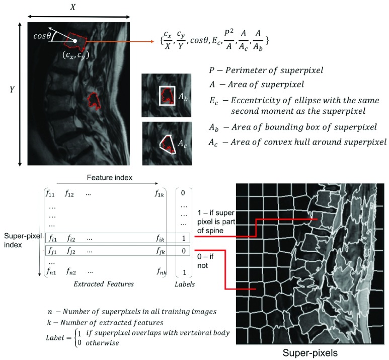
For each superpixel in the imaging data, we extract ratios that quantify the shape, the position and the orientation of the superpixel (figure 4). Next we describe each feature and the motivation behind its choice:

• Position and Orientation Features:

  • •
    We compute , the centroid of each superpixel and divide them by the corresponding maximal dimension of the image. We also compute the orientation of each superpixel (as the cosine of the angle between the X-axis and the major axis of the ellipse that has the same second-moments as superpixel) and it’s eccentricity (the ratio of the focal distances of the same ellipse). Note that the features described thus far use the distinct dichotomy that exists between computer vision and medical image analysis. While the proposed features are neither translationally nor rotationally invariant, they are highly relevant in medical image analysis. Lumbar sagittal MR images of the spine are generally acquired by placing the patient in a supine position in the bore of a scanner and the scanning is performed in a very specific manner by the technician. Thus, unlike generic computer vision problems, we can be certain that the medical image is acquired in a standardized, centered frame that contains the entire region of interest. For instance, unlike an image of a car found in a regular computer vision database containing cars, medical images are generally captured in a manner such that the lumbar vertebral bodies are placed near the center of the acquisition in a particular orientation and no occlusion. The availability of this standardization in medical image analysis is what the centroidal and orientation features proposed above capitalize upon. superpixels corresponding to vertebral bodies tend to be oriented in a specific manner in the clinical MR images. Thus, position and orientation features alone yield powerful markers for identifying vertebral superpixels.
• Complexity Features:

  • •
    : While medical MR images may be acquired in a specific frame and orientation, other challenges exist in medical imaging that do not exist in computer vision. For example color information is absent and intensity values are relative (in MR). Additionally, training data for image segmentation comes at a high cost (manual segmentation). These factors make shape based feature engineering an attractive proposition. Thus, we incorporate three shape based features into our learning enegine. The first is ratio of the square of the perimeter to the area is a crude measure of border complexity/fractal dimension of a superpixel. A superpixel with a small area, but an extremely complex boundary is unlikely to be vertebral superpixel. We expect the vertebral superpixels to be roughly square. Hence the value of this feature is expected to stay bounded. This intuition functions well in real data wherein this single feature can often distinguish between vertebral and non vertebral in a given image.
  • •
    : Solidity is the ratio of the area of the superpixel to the area of its convex hull. Since we expect the vertebral superpixel to be roughly convex we expect this value to be close to one. Extent is the ratio of the area of the superpixel to the area of the bounding box. Again, we expect this to be higher for vertebral superpixels due to the characteristic square shaped rendering of vertebral bodies in saggital MR images.

Note that we do not use superpixel intensities in defining the feature vector. The features used are purely geometry based. The combination of these features in conjunction with a suitable machine learning classifier may be used to distinguish superpixels corresponding to vertebrae from those that do not. Indeed, this is the intuition behind our approach. Yet, as stated before, note that we still rely on the accuracy of the underlying superpixel generation technique to yield at least one superpixel that corresponds to each vertebral body. This is a difficult task to achieve given that the superpixel generation problem itself is a highly non-convex one. While, it is difficult to rely on a single algorithm running at a given parameter setting to yield one superpixel per vertebral body, running multiple algorithms or even the same algorithm at several parameter settings effectively overcomes this issue, thus yielding a multi-parameter ensemble. The idea is inspired by similar models that were used in climate prediction in the early 21st century [22], [27].

FIGURE 4.

Feature extraction with superpixels. We extract six ratios to construct a feature vector from each superpixel. These ratio ultimately quantify shape, position and orientation of the specific super pixel. Training labels are generated based on the degree of overlap between a specific superpixel and manually labeled vertebral segments. When there is no overlap between a superpixel with any manually segmented vertebral region, the label corresponding to the feature extracted from the superpixel is 0, otherwise it is 1.

1). Training

To elucidate the training process further, let denote the training data set with individual ’s representing patient scans. Thus, we have training scans. We denote by describes a pre-chosen superpixel generation mechanism. Further, lets us denote by the possible/chosen set of parameters we can use for the superpixel algorithm. Given a specific parameter setting and image the super-pixel generator can generate a set of super-pixels denoted as .

The collective of all superpixels for a particular parameter setting , we then denote by:

Thus, we generate during training the collective:

which contains for every parameter setting a set of super-pixels derived using images in the entire training set. The next step is to extract the proposed features from each . We denote the feature extraction mechanism by . the feature extraction works on a superpixel to extract a ‘feature vector’ as explained in section II-D. Thus, at every parameter value we obtain a matrix in where denotes the total number of super-pixels in the set and is the dimensionality of the feature extracted. We define:

and we define the collective :

Note that each represents a unique set of features extracted from the superpixels in the corresponding . For each features corresponding to super-pixels that overlap with manually segmented vertebral bodies with a Dice score of greater than 0.85 are labeled ‘1’ and those that do not are labeled ‘0’. Thus, we have one of labeling for each . The collective is defined by:

The next step is to apply a machine learning model. We use the random forest classifier for this purpose. Now, for each super-pixel set the vast majority of super-pixels are background and a very small subset are actually vertebral bodies. Furthermore, only super-pixels that overlap with vertebral bodies (Dice score > 0.85) are labeled ‘1’ and all others are labeled zero. This creates, what is known in machine learning parlance, a highly unbalanced dataset. Amongst hundreds of super-pixels generated per image, 5 to 6 are vertebrae (labeled +1) and all others are negative samples (labeled 0). Ensemble methods such as the Random Forest (RF) [12] are better suited to handle such dataset imbalance. This is partly because they ultimately train classifiers on smaller subsets and then aggregate them by simple majority voting. Each smaller subset is likely to be more balanced due to the necessity of selecting positive as well as negative samples during the training process. Consequently, the random forest classifier naturally handles dataset imbalance, unlike competing techniques such as SVMs wherein carefully designed hard negative mining needs to be used to achieve a similar effect. Furthermore, each tree in a random forest represents a simpler model with fewer parameters as compared to a relatively complex alternatives such as deep neural networks, which can severely over fit when dataset sizes are smaller. Hence, we train random forests models to distinguish feature vectors that can identify super-pixels corresponding to vertebral bodies :

The collective of models is the trained multi-parameter ensemble model:

2). Segmentation

Given a newly acquired scan, denoted by , the procedure to segment this scan involves the following steps in a manner similar to that used in the training process. First, we run the superpixel algorithm with each parameter in the set to obtain the super-pixel sets:

Next the collective of super-pixels for all possible parameter values is formed:

Next, we extract features :

Each of these feature sets extracted from the test image are paired with the corresponding random forest classifier to discriminate super-pixels that are highly likely to have captured vertebral bodies faithfully, from background super-pixels. Thus, a candidate segmentation is produced, which may have segmented only a small subset of all the vertebral bodies in the image, but segmented these with high accuracy.

The final segmentation is the n obtained as:

III. Results

A. Procedure

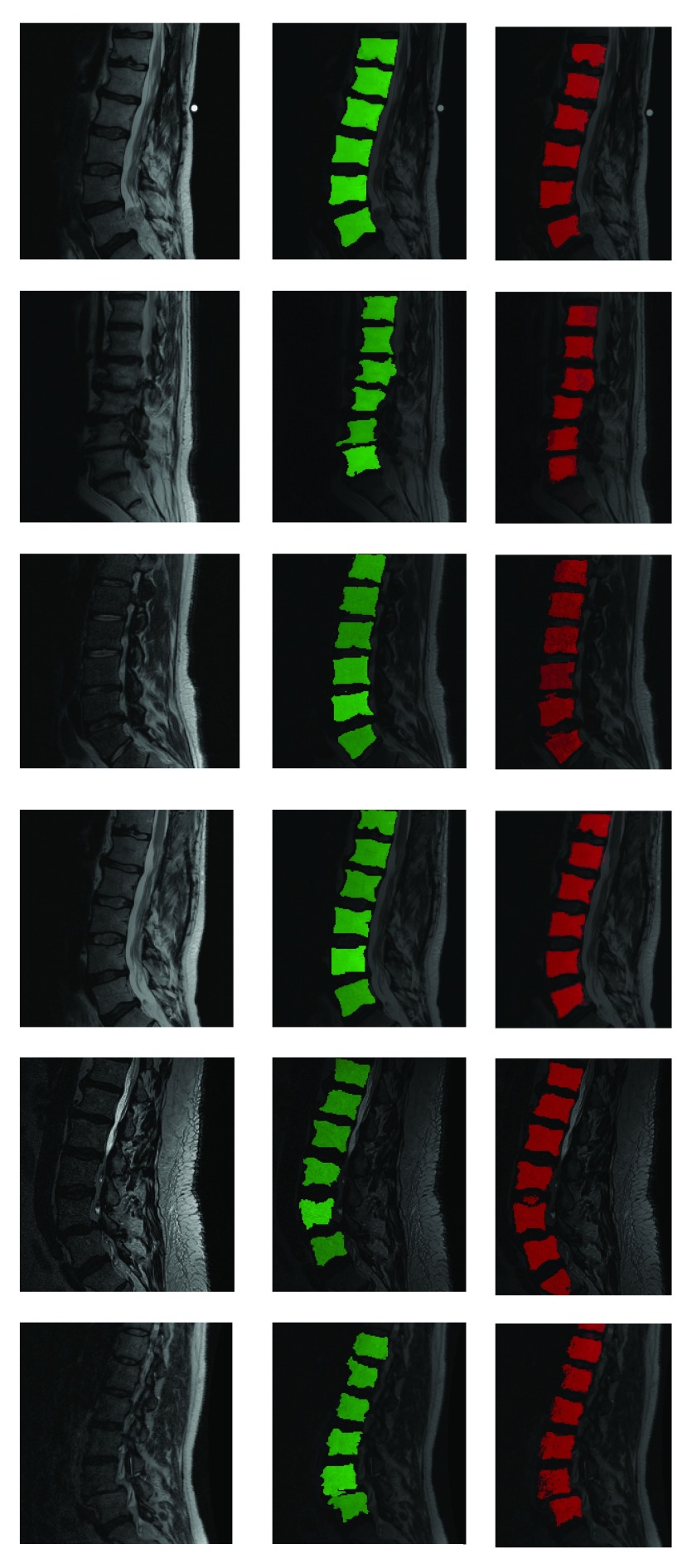
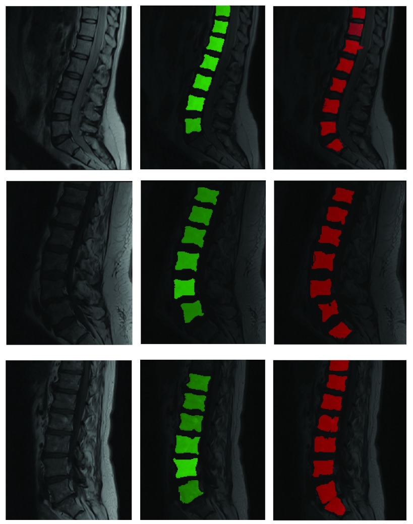
The Felzenswalb superpixel technique produces distinct results based on the specific parameter values used. The main parameter of interest while using this technique is the ‘k or the scale parameter described in [10]. In our experiments we varied the scale between 30 and 100 with intervals of 5. At lower values of scale (near 30) the algorithm divides the vertebral body into multiple sub-regions. At scales close to 100 more than one vertebral body tends to be grouped into a single superpixel. At some optimal scale value a super-pixel may appear such that it precisely segments the vertebral body. This optimal ‘scale value’ varies from one vertebral body to the next and from one image slice to the next. However, by training a classifier to identify a superpixel that adheres to a vertebral body at every possible scale value, we can capture all vertebral bodies in all slices despite any variation involved. False positive elimination was performed using a centrality measure labeling inter-slice consistency of superpixels detected as vertebral bodies of the same patient image. To refine the super-pixels picked out by the random forest, we applied a limited post-processing protocol that was designed to force the super-pixels identified to exactly correspond to gray scale edges in the original intensity image. This step consisted of identifying a two pixel thick morphological boundary around each super-pixel and adjusting super-pixel boundaries using a localized intensity clustering. As such, we did not find the post-processing to substantially improve the dice scores at p-value threshold of 0.05. Hence we have reported Dice score metrics using post-processing as well as without it in the results. As stated earlier we trained our method using 6 manually labeled sagittal T2-MRI scans and used it to segment vertebrae on 42- T2 and 15 -T1 MRI scans. The six cases used for training all came from a single acquisition center but varied in terms of acquisition/relaxation times. Even though the T2-MR scans used for validating the trained model used were obtained at more than 5 centers with varying acquisition protocols and in the presence of gross pathology, our technique produced qualitatively reasonable segmentation as shown in figures 5 and 7. In the following section we describe both qualitative and quantitative analyses of our results.

FIGURE 5.

Fully automatic segmentation of lumbar vertebrae from T2-MR scans from in spite of acquisition and pathology induced variation. Red indicates automated segmentation and green indicates manual segmentation. Note the presence of dislocation in the second row from the top and severe disk degeneration in the case in the bottom row. Further note the substantial variation in noise and bias across the cases and that not all vertebral bodies are perfectly square in shape either.

FIGURE 7.

Segmentation of T1 scans using model learnt from T2 scans. Green is manual and red is automated.

B. Segmenting Vertebrae on T2 Images After Training on T2 Images with Different Acquisition Parameters and Pathology

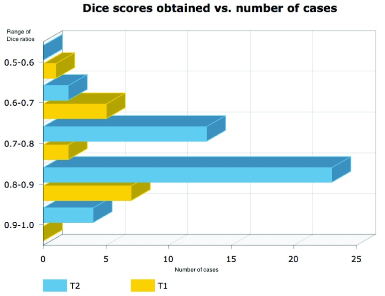
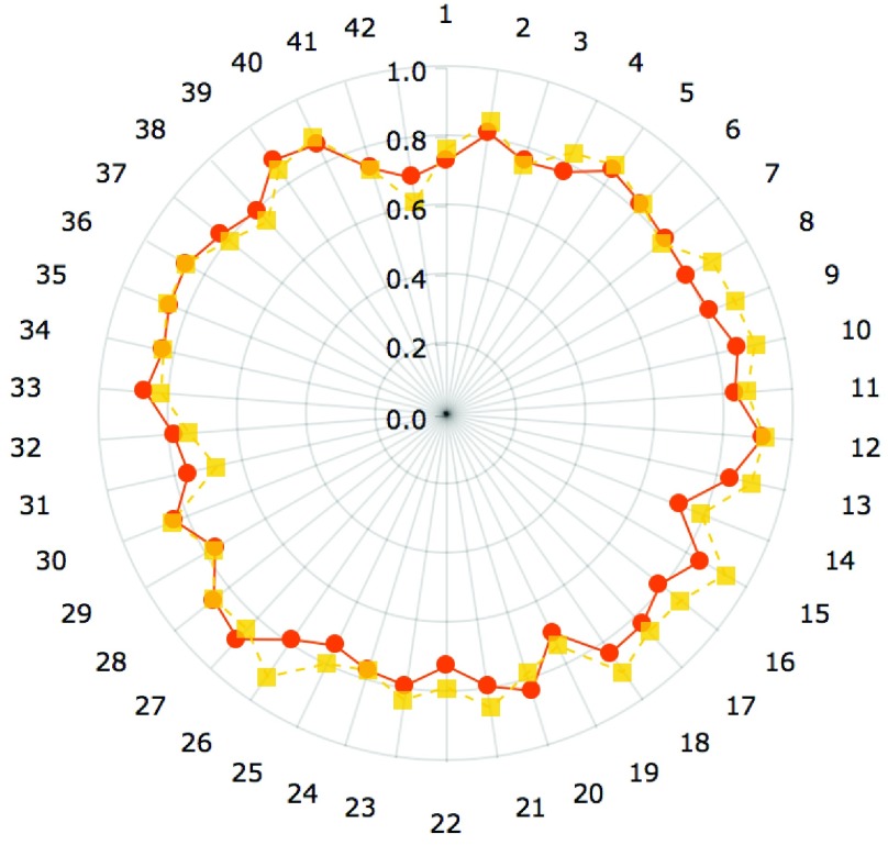
Results shown in figures 5 and 6 demonstrate the performance of our technique in segmenting vertebral bodies in real clinical data. In figure 5 we highlight the degree of variation involved in clinical data labeled ‘T2’ that is seen at a given spine center. This demonstrates the challenge that faces all computer aided diagnosis methods, if they are ever to be truly useful in the clinical setting. Specifically, the case shown in the second row of figure 5 has severe disk degeneration, obscuring the border between the vertebra. The case in row 5 is scanned with a protocol that results in an unusually bright signal in the spinal cord while relatively noisy signal in the vertebral bodies while the overall signal is heavily suppressed in the MR image in the third row. Since, we rely on superpixels computed at several parameter values followed by shape based classification ensembles, we can overcome this tremendous variability in the imaging data and present our surgeons with a clinically usable system. To quantitatively validate our technique, we manually segmented each of our 42 validation scans and compared the manual segmentations to automatic segmentations using the Dice overlap measure. Figure 6 shows the distribution of Dice coefficients. Figure 8 shows a polar plot of Dice coefficients achieved in all 42 test cases. Note that in majority of the cases the dice coefficient is > 0.8. The mean Dice score after is in spite of the tremendous variation in the data set.

FIGURE 6.

Histogram of dice scores computed by comparing automated segmentation produced using parameter ensembles to manual delineations of vertebral bodies on T2 (blue) and T1 (yellow) images.

FIGURE 8.

Dice coefficients comparing manual and automated segmentations on T2 MR scans with postprocessing(yellow) and without post-processing (orange).

C. Training on T2-Images and Segmenting on T1-Images

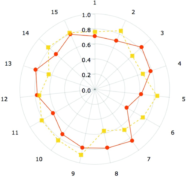
The robustness of the learning method presented can also be demonstrated by showing how well the model trained on T2-MR images can segment T1-MR scans (figure 7). Although, the results on T1-images are not as accurate as the ones on T2-images (mean dice coefficient of 0.75), they clearly demonstrate the robustness of the learning machine proposed. Figures 6 and 9 present the quantitative picture of how automated segmentations compare to manual ones. To the best of our knowledge, this type of ‘cross modality learning’ is a first in spine segmentation literature.

FIGURE 9.

Dice coefficients comparing manual and automated segmentations on T1 MR scans (using model trained on T2 scans) with post-processing(yellow) and without post-processing (orange).

D. Comparison with Alternative Methods

In order to further convince the reader of the robustness of our technique as compared to competing techniques we present in this sub-section a comparison between the proposed methodology and comparable existing methods from segmentation literature. The three methods that we compare against include watershed transform driven segmentation [4], [5], [13], [30], the related random walker based segmentation [12] and active shape modeling. For both watershed and random walker methods we initialize a pixel region in the center of each vertebral body as vertebral body markers and use regions outside a pixel box around the vertebral center as a background marker. For Active shape modeling (ASM) [6], [24] we used a shape initialization that was defined individually for each vertebral body. A 2D ASM was trained using 30 vertex points to VBs in the training data. We fit individual 2D-ASMs to each VB on each slice in the test data. The results of our comparative experiments are summarized in table 1.

TABLE 1. Comparison Between Dice Scores (DSC) Proposed Ensemble Segmentation and Standard Segmentation Techniques.

	Proposed method	Watershed	Random walker	Active shape models
Mean DSC	0.849	0.741	0.723	0.585
Std. dev. DSC	0.0497	0.106	0.108	0.219
Max. DSC	0.916	0.913	0.886	0.907
Min. DSC	0.718	0.316	0.293	0.127

While standard techniques are indeed comparable on certain cases as evidenced by the ‘Max DSC’ row, the proposed approach does much better on the ‘Min DSC’ row and presents us with a substantially lower standard deviation. This is because when the super-pixel algorithm is run for a large number of parameter settings it tends to generate a wide choice of delineations for the succeeding random forest classifiers. Under such a paradigm the random forest can easily reject any segmentation that might be slightly less accurate. A typical segmentation approach that relies on a two stage paradigm of ‘detection’ followed by the application of a standard ‘segmentation’ method [14], [18], [19], [31], does not have this flexibility since out of the box segmentation algorithms are applied post the detection step yielding a less flexible overall approach.

IV. Discussion

A. The Effect of Post Processing

We indicated in the results section that we apply a series of simple post processing steps to refine the initial superpixel segmentations. While the post processing definitely increases the mean Dice ratio for both T2 and T1 segmentations the gains are made at the cost of slightly higher variation in the scores themselves. To quantify the impact of the post processing we show dice scores obtained with and without post-processing on both T2 and T1 MR test scans. Figure 8 indicates the effect of post-processing in case of the T2 images. The mean Dice score before the post-processing was 0.81 which was slightly lower than after it 0.83. However the standard deviation in the Dice scores after applying the post-processing was 0.06 which was slightly higher than the standard deviation obtained before applying it, which was 0.05. We surmise that this improvement may be due to the fact that local intensity based algorithms such as watersheds are better able to deal with intensity contrast reduction effected by supressing the water related signals in the T2 sequence. Yet, the difference in the means as measured by a t-statistic not statistically significant between post processed and non post-processed images (t-statistic=1.37, p-value=0.18). Similar trends were seen in the T1 segmentation results. Figure 9 shows a polar plot comparing dice ratios for T1 images before and after post-processing. In the case of T1-MRI segmentation significant difference was not observed between dice scores computed before and after post processing. For these images the mean Dice scores before post processing was 0.737 and after it was 0.747. A t-test for difference between the means was not significant (t-statistic: 0.297, p-value 0.767). While we have retained the post-processing due to the mean increase in Dice coefficients, with the maximum increase in an individual case being 0.12, additional work is required to identify which specific cases are likely to generally benefit from post-processing.

B. Qualitative Comparisons with Other Methods Used in Brain and Bone Imaging

The use of standard pipeline (N4+ Histogram equalization + Rigid registration) for image and pixel size normalization is often the first step in the automated segmentation of many anatomical structures including brain, breast, liver and prostate. The registration step is often the first step towards atlas building and machine learning for such structures as it normalizes the pixel spacing and intensity heterogeneity. However, this generic protocol may not be well suited for preprocessing in clinical spine imaging. In figure 10, we illustrate the application of rigid registration with FSL’s Flirt tool to spine imaging data [16].

FIGURE 10.

Result of standard pipeline using N4+histogram equalization+rigid registration. Template (left), subject (center) and registered subject (right).

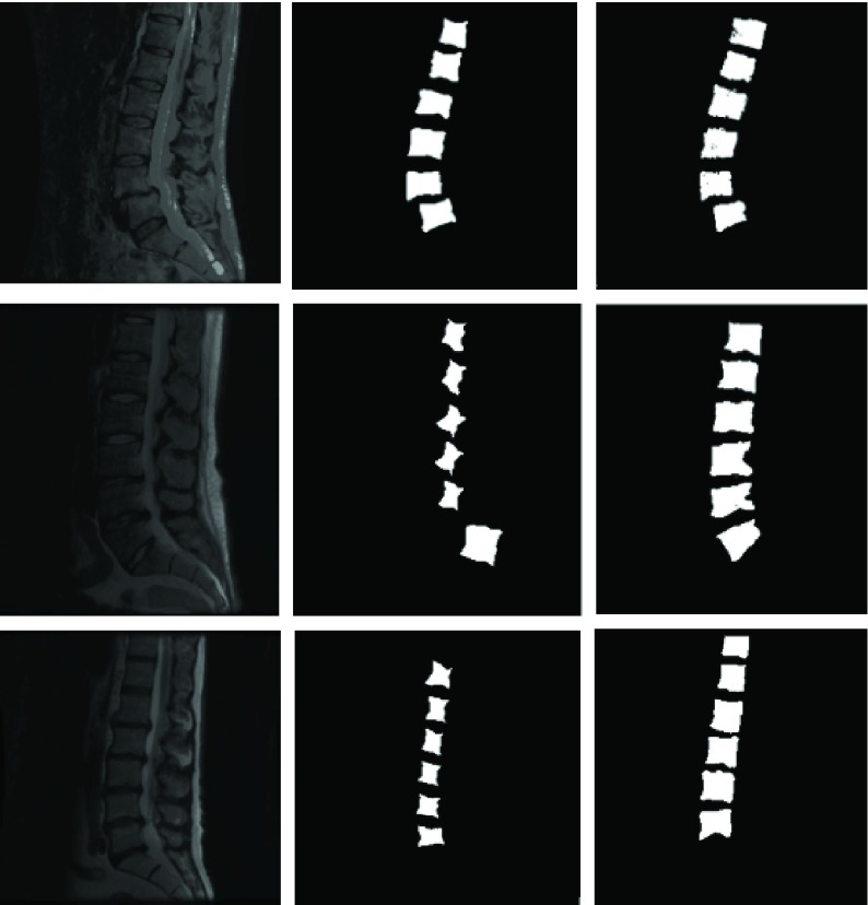
Figure 10 shows that the algorithm rotates the image out of the sagittal plane to match it with the template. While registration fails, this example also elucidates the necessity for further research into the development of image registration methods for spine MR data. Standard segmentation methodology used in bone image analysis typically revolves around shape modeling. The use of shape modeling in vertebral body detection/segmentation is reasonable. Hence we presented results using related techniques in section III-D. We further elaborate on the qualitative aspects of these results in this section. Figure 11 shows how the active shapes based segmentation performs on two different cases in our dataset. In the first case (row) the ASM model works in a fashion comparable to the proposed technique and indeed produces a reasonable segmentation. In the second row it seems to fail. This failure is likely due to the presence of strong edges inside the vertebral bodies in the second image in addition to an atypical suppression of intensities near the top of the image. Despite the challenge, the performs a reasonable segmentation. Given both images, a human physician would be expected to accurately delineate where the vertebral bodies are. Our ensemble learning based technique mimics this ability.

FIGURE 11.

Original images (left), Segmentation using active shapes (center) and segmentation using proposed methodology(right). Top row represents a case where ASM segments vertebral bodies satisfactorily. Middle row and Bottom row show cases where ASM inaccurately estimates rotation (middle row) or scale (bottom row) parameters associated with the model.

C. Variation in Accuracy with Variation in Number of Base Learners

As stated earlier, in the experiments presented, we varied the scale parameter of the Felzenswalb superpixel algorithm between 30 and 100 in intervals of 5.

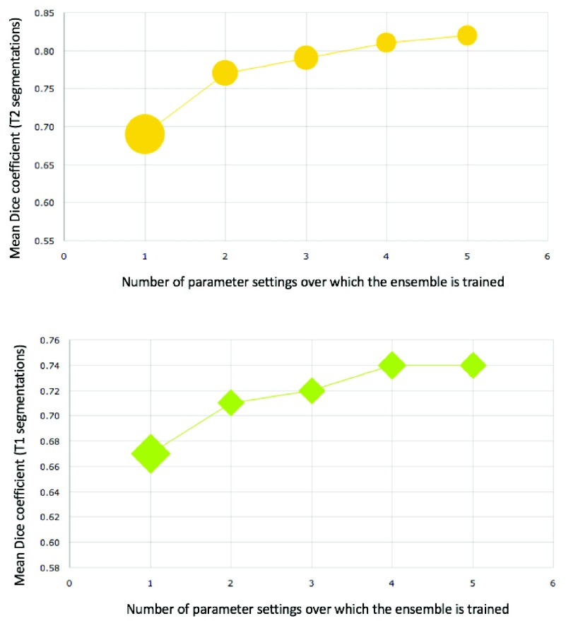
This choice was made by looking at a single test image and observing that below 30 superpixels generated approach the size of pixel spacing and above 100, they unusably large (encompassing the entire spine). Yet, the question of how best to sample the space of parameters remains unaddressed in the current work. In general generating superpixels with a smaller range of parameter settings, in the multi-parameter ensemble leads to worse results. This is documented in figure 13.

FIGURE 13.

Variation of Dice score within the segmentations produced for T2 (top) and T1 (bottom) images with increasing number of independent parameter settings used for constructing ensemble. Initially the addition of base learners at different parameter settings improves Dice ratios substantially while reducing variance (indicates by marker width) amongst the Dice ratios. As more base learners are added the increase in performance is relatively less pronounced, but the decrease in variance is substantial.

D. Training with Minimal Amount of Data

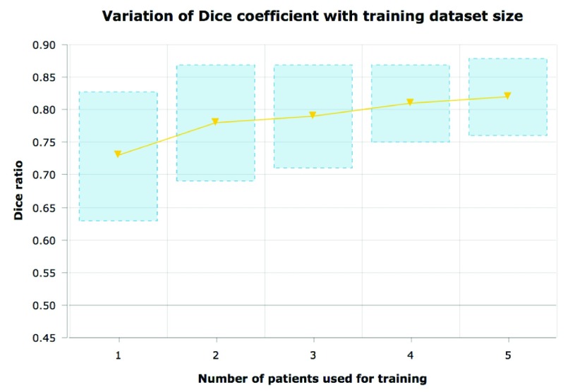
Note that all the results described above were obtained using a very small training data set (namely 6 cases). This elucidates the fact that we can train robust and powerful segmentation methods using a minimal amount of training data, albeit at enormous computation costs. However, computational costs will be progressively less important in the future. The ability to generalize to large datasets by learning from a small dataset is a strength that will be more valuable as datasets get larger in the future. The proposed method can improve with increased training data. We show results obtained by re-training the algorithm on a fewer number of training data points (figure 14). While more labeled data improves performance, we perform reasonably well even when trained using just 3 manually labeled cases. Generally training a standard object detection framework (such as the Viola -Jones detector [25]) requires a very large and diverse training data set that captures the shape, pose and intensity variation of the object being detected. One of the key problems in medical image analysis is the limited availability of such labeled training data. Thus, a similar multi-parametric approach could potentially be useful for segmenting other organs/regions of interest in clinical imaging data in conjunction with this or other superpixel centric methods. While there is limited work on using multi-parameter ensembles in medical image segmentation, the thriving field of multi-atlas brain image registration draws upon similar principles [8].

FIGURE 14.

Variation of Dice score within the segmentations produced for T2 images with increasing number of training subjects. As expected increased more training data leads to better accuracy and lesser variation in the predicted Dice score values.

E. Could Parameter Optimization Replace Multi-Parameter Ensembles

Another approach to segmenting data that is obtained under a widely varying set of parameters could potentially utilize the TR/TE values themselves to modify the segmentation algorithm. For instance, one may be able to remedy the failure of the active shape models shown in Fig 11 by a)’training’ a dictionary of shape models using images acquired at numerous distinct TR/TE settings and then b) performing segmentation on a patient image by choosing a shape model which matches the patient acquisition in terms of TR/TE. While such an approach might be possible, it is unclear if and how such an approach would deal with variation within a single image itself due to factors such as acquisition bias or pathology. Despite the challenges, this remains an interesting avenue of research that requires further exploration.

F. Robustness and Segmenting CT Data

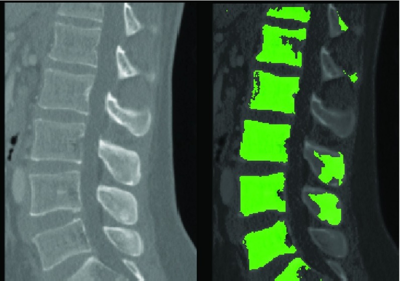
While the difference between T1 and T2 MRI is stark, a human clinician who has seen the spine on T2-MR will be able to identify at least some of the relevant structures on T1-MRI. The proposed method mimics this ability. While the primary thrust of the study was MR imaging for exploratory purposes we attempted to segment a CT image obtained from a publicly available database of CT images using the ‘learnt’ model. The result is presented in figure 12. The proposed method is able to identify and segment vertebral bodies on CT even after training solely on MR images.

FIGURE 12.

Segmenting a CT image using a model trained on T2-MR images.

G. A Note on Pathology

An important aspect of our data set was that it contained a large number of pathological cases. Since, the data set was directly collected from an active spine clinic, it was unlike most data sets that have been employed in the literature, and contained cases with some type of pathology. Existing literature, tends to utilize scans obtained from normal subjects for segmentation. Shapes of vertebral bodies cannot be assumed to be consistent in the presence of pathology. This is well illustrated by images in figures 5 and 6. In spite of this variation, the proposed superpixel centric technique is able to robustly delineate anatomy. Further research will be required to modify/evaluate if competing techniques can achieve such an outcome.

V. Conclusion

In conclusion we reiterate that we have constructed a machine learning based system for segmentation of vertebral bodies on clinicalMRimages of the lumbar spine. The primary methodological differentiators of our technique from previous work is the use of superpixels based multi-parameter ensemble learning. However, the primary motivation of the work is to create a system that can be used segment lumbar vertebrae reliably even in the presence of tremendous variation in the scanning protocol and comparable variation due to the presence of pathology. The fact that our technique works in the presence of substantial variation in the scanning parameters in T2 images is significant. The fact that it can learn using a relatively small training set and use a model trained using T2-images to segment vertebrae on T1-images establishes the robustness of the proposed learning methodology. Future work will focus on reducing the time required for training and segmenting vertebrae using the proposed methodology, validation on larger data sets and the development of a live web based application where spine surgeons and other clinical practitioners can use the system to augment diagnostic decisions.

Biographies

Bilwaj Gaonkar received the Ph.D. degree from the Department of Biomedical Engineering, University of Pennsylvania, focused on extracting information from big data in neuroimaging. He is a Post-Doctoral Scholar with the Department of Neurosurgery, University of California at Los Angeles. He currently leads several projects aiming to leverage clinical imaging and informatics data to improve medical decision making. His research lies at the intersection of image processing, machine learning, and clinical informatics.

Yihao Xia received the master’s degree in electrical engineering from the University of Southern California, Los Angeles, CA, USA, in 2017, where he is currently pursuing the Ph.D. degree with the Laboratory of Neuro Imaging. His current research interests include biomedical image analysis, image segmentation, and machine learning.

Diane S. Villaroman received the B.S. degree in neuroscience from the University of California at Los Angeles (UCLA). She utilizes different programming languages, such as JavaScript, C-sharp, and Python, to integrate technology into medical practices. She joined the Neurosurgery Department, UCLA, in 2016. Her current research includes studies on spinal medical image analysis, brain mechanisms underlying real-world ambulatory behaviors, and medical education via virtual reality.

Allison Ko is currently pursuing the master’s degree in linguistics and computer science with the University of California at Los Angeles. Her current research interests include image processing, computational linguistics, and natural language processing.

Mark Attiah received the M.D. degree from the University of Pennsylvania in 2015. He is a Resident Physician of Neurosurgery with the University of California at Los Angeles. His current interests include the application of machine learning techniques to clinical decision making using big data and also interested in spine imaging and the development of image driven quantitative methods of clinical decision making.

Joel S. Beckett received the M.D. and M.H.S. degrees from Yale University in 2013. He was a former Doris Duke Clinical Research Scholar. He is a Neurosurgical Resident with the University of California at Los Angeles. He seeks to utilize modern imaging and computer vision techniques to streamline diagnoses and procedural planning in neurosurgery.

Luke Macyszyn is an Assistant Professor-in-Residence with the Department of Neurosurgery and Orthopedics with the University of California at Los Angeles (UCLA). He has studied various neurological disorders over the past ten years, including cerebral vasospasm, imaging phenotypes in brain cancer, and advanced imaging techniques for white matter tractography. More recently, at the University of Pennsylvania, he was involved in the application of advanced imaging techniques to brain cancer, correlating advanced neuroimaging phenotypes with proteomics in human gliomas and characterizing edema/infiltration in white matter tissue to improve tractography. He developed a unique algorithm that can predict the region of recurrence in newly diagnosed glioblastoma and modeled the effect of edema on brain tractography, culminating in a clinical package for improved perioperative planning. He currently uses his extensive knowledge of image analysis, processing and machine learning at UCLA to develop automated algorithms for spinal image segmentation and create quantitative imaging biomarkers of spinal pathology. He aims to develop specific biomarkers for degenerative lumbar disease to standardize diagnosis and augment treatment selection to improve patient outcomes.

References

- [1].Achanta R., Shaji A., Smith K., Lucchi A., Fua P., and Süsstrunk S., “SLIC superpixels compared to state-of-the-art superpixel methods,” IEEE Trans. Pattern Anal. Mach. Intell., vol. 34, no. 11, pp. 2274–2282, Nov. 2012. [DOI] [PubMed] [Google Scholar]
- [2].Alomari R. S., Corso J. J., and Chaudhary V., “Labeling of lumbar discs using both pixel- and object-level features with a two-level probabilistic model,” IEEE Trans. Med. Imag., vol. 30, no. 1, pp. 1–10, Jan. 2011. [DOI] [PubMed] [Google Scholar]
- [3].Ayed I. B., Punithakumar K., Garvin G., Romano W., and Li S., “Graph cuts with invariant object-interaction priors: application to intervertebral disc segmentation,” in Information Processing in Medical Imaging. Berlin, Germany: Springer, 2011, pp. 221–232. [DOI] [PubMed] [Google Scholar]
- [4].Chevrefils C., Cheriet F., Aubin C.-É., and Grimard G., “Texture analysis for automatic segmentation of intervertebral disks of scoliotic spines from MR images,” IEEE Trans. Inf. Technol. Biomed., vol. 13, no. 4, pp. 608–620, Apr. 2009. [DOI] [PubMed] [Google Scholar]
- [5].Chevrefils C., Chériet F., Grimard G., and Aubin C.-E., “Watershed segmentation of intervertebral disk and spinal canal from MRI images,” in Image Analysis and Recognition. Berlin, Germany: Springer, 2007, pp. 1017–1027. [Google Scholar]
- [6].Cootes T. F., Taylor C. J., Cooper D. H., and Graham J., “Active shape models-their training and application,” Comput. Vis. Image Understand., vol. 61, no. 1, pp. 38–59, 1995. [Google Scholar]
- [7].Corso J. J., Alomari R. S., and Chaudhary V., “Lumbar disc localization and labeling with a probabilistic model on both pixel and object features,” in Medical Image Computing and Computer-Assisted Intervention–MICCAI. Berlin, Germany: Springer, 2008, pp. 202–210. [DOI] [PubMed] [Google Scholar]
- [8].Doshi J., Erus G., Ou Y., Gaonkar B., and Davatzikos C., “Multi-atlas skull-stripping,” Acad. Radiol., vol. 20, no. 12, pp. 1566–1576, 2013. [DOI] [PMC free article] [PubMed] [Google Scholar]
- [9].Egger J.et al. , “Square-Cut: A segmentation algorithm on the basis of a rectangle shape,” PLoS One, vol. 7, no. 2, p. e31064, 2012. [DOI] [PMC free article] [PubMed] [Google Scholar]
- [10].Felzenszwalb P. F. and Huttenlocher D. P., “Efficient graph-based image segmentation,” Int. J. Comput. Vis., vol. 59, no. 2, pp. 167–181, Sep. 2004. [Google Scholar]
- [11].Gaonkar B., Shu L., Hermosillo G., and Zhan Y., “Adaptive geodesic transform for segmentation of vertebrae on CT images,” Proc. SPIE, vol. 9035, p. 903516, Mar. 2014. [Google Scholar]
- [12].Grady L., “Random walks for image segmentation,” IEEE Trans. Pattern Anal. Mach. Intell., vol. 28, no. 11, pp. 1768–1783, Nov. 2006. [DOI] [PubMed] [Google Scholar]
- [13].Grau V., Mewes A. U. J., Alcaniz M., Kikinis R., and Warfield S. K., “Improved watershed transform for medical image segmentation using prior information,” IEEE Trans. Med. Imag., vol. 23, no. 4, pp. 447–458, Apr. 2004. [DOI] [PubMed] [Google Scholar]
- [14].Huang S.-H., Chu Y.-H., Lai S.-H., and Novak C. L., “Learning-based vertebra detection and iterative normalized-cut segmentation for spinal mri,” IEEE Trans. Med. Imag., vol. 28, no. 10, pp. 1595–1605, Oct. 2009. [DOI] [PubMed] [Google Scholar]
- [15].Jenkinson M., Beckmann C. F., Behrens T. E., Woolrich M. W., and Smith S. M., “FSL,” NeuroImage, vol. 62, no. 2, pp. 782–790, 2012. [DOI] [PubMed] [Google Scholar]
- [16].Kang Y., Engelke K., and Kalender W. A., “A new accurate and precise 3-D segmentation method for skeletal structures in volumetric CT data,” IEEE Trans. Med. Imag., vol. 22, no. 5, pp. 586–598, May 2003. [DOI] [PubMed] [Google Scholar]
- [17].Law M. W., Tay K., Leung A., Garvin G. J., and Li S., “Intervertebral disc segmentation in mr images using anisotropic oriented flux,” Med. Image Anal., vol. 17, no. 1, pp. 43–61, 2013. [DOI] [PubMed] [Google Scholar]
- [18].Neubert A.et al. , “Automated detection, 3D segmentation and analysis of high resolution spine mr images using statistical shape models,” Phys. Med. Biol., vol. 57, no. 24, p.8357, 2012. [DOI] [PubMed] [Google Scholar]
- [19].Peng Z., Zhong J., Wee W., and Lee J.-H., “Automated vertebra detection and segmentation from the whole spine mr images,” in Proc. IEEE-EMBS 27th Annu. Int. Conf. Eng. Med. Biol. Soc., Sep. 2006, pp. 2527–2530. [DOI] [PubMed] [Google Scholar]
- [20].Schwarzenberg R., Freisleben B., Nimsky C., and Egger J., “Cube-Cut: Vertebral body segmentation in MRI-data through cubic-shaped divergences,” PloS one, vol. 9, no. 4, p. e93389, 2014. [DOI] [PMC free article] [PubMed] [Google Scholar]
- [21].Sled J. G., Zijdenbos A. P., and Evans A. C., “A nonparametric method for automatic correction of intensity nonuniformity in MRI data,” IEEE Trans. Med. Imag., vol. 17, no. 1, pp. 87–97, Feb. 1998. [DOI] [PubMed] [Google Scholar]
- [22].Stainforth D. A.et al. , “Uncertainty in predictions of the climate response to rising levels of greenhouse gases,” Nature, vol. 433, no. 7024, pp. 403–406, 2005. [DOI] [PubMed] [Google Scholar]
- [23].Tustison N. J.et al. , “N4ITK: Improved N3 bias correction,” IEEE Trans. Med. Imag., vol. 29, no. 6, pp. 1310–1320, Jun. 2010. [DOI] [PMC free article] [PubMed] [Google Scholar]
- [24].van Ginneken B., Frangi A. F., Staal J. J., ter B. M. Romeny H., and Viergever M. A., “Active shape model segmentation with optimal features,” IEEE Trans. Med. Imag., vol. 21, no. 8, pp. 924–933, Aug. 2002. [DOI] [PubMed] [Google Scholar]
- [25].Viola P. and Jones M., “Rapid object detection using a boosted cascade of simple features,” in Proc. Comput. Vis. Pattern Recognit. (CVPR), vol. 1 Dec. 2001, pp. I-511–I-518. [Google Scholar]
- [26].Wang Z., Zhen X., Tay K., Osman S., Romano W., and Li S., “Regression segmentation for spinal images,” IEEE Trans. Med. Imag., vol. 34, no. 8, pp. 1640–1648, Aug. 2015. [DOI] [PubMed] [Google Scholar]
- [27].Yang Z. and Arritt R. W., “Tests of a perturbed physics ensemble approach for regional climate modeling,” J. Climate, vol. 15, no. 20, pp. 2881–2896, 2002. [Google Scholar]
- [28].Yao J., O’Connor S. D., and Summers R. M., “Automated spinal column extraction and partitioning,” in Proc. 3rd IEEE Int. Symp. Biomed. Imag., Nano Macro, Apr. 2006, pp. 390–393. [Google Scholar]
- [29].Zhan Y., Maneesh D., Harder M., and Zhou X. S., “Robust mr spine detection using hierarchical learning and local articulated model,” in Medical Image Computing and Computer-Assisted Intervention–MICCAI. Berlin, Germany: Springer, 2012, pp. 141–148. [DOI] [PubMed] [Google Scholar]
- [30].Zukić D., Vlasák A., Egger J., Hovřínek D., Nimsky C., and Kolb A., “Robust detection and segmentation for diagnosis of vertebral diseases using routine MR images,” Comput. Graph. Forum, vol. 33, no. 6, pp. 190–204, 2014. [Google Scholar]
- [31].Gaonkar B.et al. , “Automated tumor volumetry using computer-aided image segmentation,” Acad. Radiol., vol. 22, no. 5, pp. 653–661, 2015. [DOI] [PMC free article] [PubMed] [Google Scholar]