Meta‐analysis of two studies in the presence of heterogeneity with applications in rare diseases

Abstract

Random‐effects meta‐analyses are used to combine evidence of treatment effects from multiple studies. Since treatment effects may vary across trials due to differences in study characteristics, heterogeneity in treatment effects between studies must be accounted for to achieve valid inference. The standard model for random‐effects meta‐analysis assumes approximately normal effect estimates and a normal random‐effects model. However, standard methods based on this model ignore the uncertainty in estimating the between‐trial heterogeneity. In the special setting of only two studies and in the presence of heterogeneity, we investigate here alternatives such as the Hartung‐Knapp‐Sidik‐Jonkman method (HKSJ), the modified Knapp‐Hartung method (mKH, a variation of the HKSJ method) and Bayesian random‐effects meta‐analyses with priors covering plausible heterogeneity values; $\mathsf{R}$ code to reproduce the examples is presented in an appendix. The properties of these methods are assessed by applying them to five examples from various rare diseases and by a simulation study. Whereas the standard method based on normal quantiles has poor coverage, the HKSJ and mKH generally lead to very long, and therefore inconclusive, confidence intervals. The Bayesian intervals on the whole show satisfying properties and offer a reasonable compromise between these two extremes.

1. Introduction

Meta‐analyses are used to combine evidence of treatment effects from multiple studies. Since treatment effects may vary across trials due to some slight differences in study characteristics including study populations, trial designs, endpoints, and standardization of treatments, heterogeneous treatment effects are quite natural and must be accounted for to achieve valid statistical inferences. Therefore, random‐effects meta‐analysis has become the standard to combine treatment effects from several studies when the presence of between‐trial heterogeneity is suspected, which is often the case.

The standard model for random‐effects meta‐analysis assumes approximately normal effect estimates and a normal random‐effects model, the normal–normal hierarchical model (Hedges and Olkin, 1985). Based on this model, standard inference methods based on normal quantiles to construct confidence intervals for the combined effect ignore the uncertainty in the estimation of the between‐study heterogeneity and they are only valid for large numbers of trials. However, the combination of only a few studies is quite common (Davey et al., 2011; Turner et al., 2012). This is not only the case in rare diseases, but in this context it poses a particular challenge since increased levels of heterogeneity are common (Friede et al., 2016). For instance, in a recent systematic review by Crins et al. (2014) six studies on acute graft rejections and three studies on steroid‐resistant rejections were combined in random‐effects meta‐analyses to assess the efficacy and safety of Interleukin‐2 receptor antibodies for immunosuppression following liver transplantation in children. All studies were controlled, but only two were randomized as it is often the case in paediatrics. Furthermore, there were some differences between the studies with respect to their control groups and other design characteristics suggesting some degree of between‐trial heterogeneity.

For random‐effects meta‐analyses with few studies methods based on t‐distributions have been suggested (Follmann and Proschan, 1999; Hartung and Knapp, 2001a,b; Knapp and Hartung, 2003; Sidik and Jonkman, 2003). Furthermore, the use of priors covering plausible between‐trial standard deviations has been advocated when dealing with few studies (Spiegelhalter et al., 2004; Neuenschwander et al., 2010; Schmidli et al., 2014; Friede et al., 2016).

Here, we consider the special case of only two studies that has recently attracted some attention (Gonnermann et al., 2015). Examples for meta‐analyses of two studies include the summary of two pivotal studies of a clinical development programme (European Medicines Agency (EMEA), 1998, 2001; International Conference on Harmonisation of Technical Requirements for Registration of Pharmaceuticals for Human Use (ICH), 2002). As we will see when discussing several examples below, meta‐analyses of two studies are not uncommon in orphan diseases. For instance, two randomized controlled trials were included in the systematic review by Crins et al. (2014) and the Cochrane Review by Miller et al. (2012) on Riluzole in amyotrophic lateral sclerosis (ALS). In the presence of heterogeneity, however, the meta‐analysis of only two studies may be considered an unsolved problem (Gonnermann et al., 2015). Therefore, we assess here the performance of alternative approaches to real‐life examples from rare diseases and explore their characteristics in an extensive simulation study. Based on these findings we give some recommendations on how to approach the problem successfully in practice.

The paper is organized as follows. In Section 2, the statistical model is introduced and methods for frequentist and Bayesian inference are reviewed. Five examples in various rare diseases are presented in Section 3 before an extensive simulation study is presented in Section 4. In Section 5, we close with a brief discussion of the findings. In an appendix $\mathsf{R}$ code to reproduce the examples is presented.

2. Methodology

2.1. Notation and statistical model

Standard meta‐analytic models assume either a common (fixed) effect or random effects across studies. For the latter, the normal–normal hierarchical model (NNHM) is the most popular. At the first level, the sampling model assumes approximately normally distributed estimates $Y_1,\dots ,Y_k$ for the trial‐specific parameters ${\theta }_1,\dots ,{\theta }_k$

$$Y_j|{\theta }_j\sim \mathrm{N}({\theta }_j,s_j^2),j=1,\dots ,k.$$ (1)

Here, we will follow the standard assumption that treats the standard errors $s_j$ as known, although this could be relaxed if necessary. At the second level, the parameter model assumes normally distributed study effects

$${\theta }_j|\mu ,\tau \sim \mathrm{N}(\mu ,{\tau }^2),j=1,\dots ,k.$$ (2)

The between‐trial standard deviation τ determines the degree of heterogeneity across studies. If the parameter of interest is μ (rather than the study effects ${\theta }_j$), inference can be simplified by using the marginal model

$$Y_j|\mu ,\tau \sim \mathrm{N}(\mu ,s_j^2+{\tau }^2),j=1,\dots ,k.$$ (3)

The two main approaches to infer μ and the nuisance parameter τ are frequentist and Bayesian. If τ were known, frequentist and Bayesian (with a noninformative prior for μ) conclusions would be analogous. In fact, in the frequentist setting

$$\widehat{\mu }=\sum _{j=1}^k{w}_j{Y}_j/\sum _{j=1}^k{w}_j\sim \mathrm{N}(\mu ,1/w_{+}),w_j=1/\left(s_j^2+{\tau }^2\right),j=1,\dots k,$$ (4)

where $w_j$ are inverse‐variance (precision) weights, and $w_{+}={\sum }_{j=1}^k{w}_j$ is the total precision; the respective variance $1/w_{+}$ is important to construct confidence intervals for μ, as shown in Section 2.2. The Bayesian result (posterior distribution) is

$$\mu |Y_1,\dots ,Y_k\sim \mathrm{N}\left(\sum _{j=1}^k{w}_j{Y}_j/\sum _{j=1}^k{w}_j,1/w_{+}\right).$$ (5)

For unknown τ, this frequentist‐Bayesian “equivalence” breaks down, since the two approaches handle estimation uncertainty for τ differently.

2.2. Frequentist inference

For unknown τ we first consider frequentist methods to infer μ, which comprise two steps.

• (1)
  An estimate $\widehat{\tau }$ is derived, from which estimated weights ${\widehat{w}}_j=1/(s_j^2+{\widehat{\tau }}^2)$ and a corresponding estimate $\widehat{\mu }$ in (4) are obtained. Various estimators for τ have been proposed (for an overview see DerSimonian and Kacker (2007); Rukhin (2012); Veroniki et al. (2016)), the most prominent being the moment‐estimator due to DerSimonian and Laird (DL). Alternatives are the maximum likelihood (ML) estimator, the restricted maximum‐likelihood estimator (REML), and the Paule‐Mandel estimator (PM). While these estimates can differ considerably, for the special case of two trials they coincide (Rukhin, 2012). We will refer to this common estimate

  $${\widehat{\tau }}^2=\frac{{(y_1-y_2)}^2-s_1^2-s_2^2}{2}.$$ (6)

  as the DL estimate, whereby negative values are set to zero. The relationship to the other often‐used heterogeneity metric I ² is

  $$I^2=\frac{{\widehat{\tau }}^2}{{\widehat{\tau }}^2+{(s_1^2+s_2^2)}^2/2}=\frac{2{\widehat{\tau }}^2}{{(y_1-y_2)}^2}=1-\frac{{(s_1^2+s_2^2)}^2}{{(y_1-y_2)}^2}$$ (7)

  where the last equation only holds if $\widehat{\tau }>0$; if not, I ² is zero. Importantly, for two trials the chance that $\widehat{\tau }$ and I ² are zero, that is ${(y_1-y_2)}^2\le s_1^2+s_2^2$, can be high even if trials are heterogeneous $(\tau >0)$. For example, four of the five applications in Section 3 estimate τ as zero although the context suggests otherwise.
• (2)
  A confidence interval for μ is then derived. Here, we will investigate three methods.

  • (i)
    The simplest approach, which was proposed in the seminal paper by DerSimonian and Laird (1986), uses the following normal approximation

    $$(\mathrm{DL}-\mathrm{Normal})\widehat{\mu }\pm {\widehat{\sigma }}_{\mu }{z}_{(1-\alpha /2)},\mathrm{where}{\widehat{\sigma }}_{\mu }^2=1/\sum _{j=1}^k{\widehat{w}}_j,$$ (8)

    and $z_p$ is the p‐quantile of the standard normal distribution. This method is known to be problematic for small k, since it ignores the uncertainty of $\widehat{\tau }$ and will therefore give too narrow confidence intervals and inflated type‐I errors.
  • (ii)
    Various improvements using a t‐distribution with $k-1$ degrees of freedom and alternative estimators for ${\sigma }_{\mu }$ have been proposed (Hartung and Knapp, 2001a,b; Knapp and Hartung, 2003; Sidik and Jonkman, 2003). The HKSJ confidence interval is given by

    $$\begin{array}{c}\hfill (\mathrm{DL}-\mathrm{HKSJ})\widehat{\mu }\pm {\stackrel{\sim }{\sigma }}_{\mu }{t}_{k-1,(1-\alpha /2)},\mathrm{where}\\ \hfill {\stackrel{\sim }{\sigma }}_{\mu }^2=\frac{1}{k-1}\sum _{j=1}^k{\widehat{w}}_j{(y_j-\widehat{\mu })}^2/\sum _{j=1}^k{\widehat{w}}_j,\end{array}$$ (9)

    and $t_{k-1,(1-\alpha /2)}$ is the $(1-\alpha /2)$‐quantile of the Student‐t distribution with $k-1$ degrees of freedom. It works well for any number of studies if study‐specific standard errors $s_j$ are of similar magnitude. Otherwise, coverage probabilities can be below the nominal level.
  • (iii)
    To address the limitations of the HKSJ method, a modified interval

    $$(\mathrm{DL}-\mathrm{mKH})\widehat{\mu }\pm {\sigma }_{\mu }^{★}{t}_{k-1,(1-\alpha /2)},\mathrm{where}{\sigma }_{\mu }^{★}=max\{{\widehat{\sigma }}_{\mu },{\stackrel{\sim }{\sigma }}_{\mu }\}$$ (10)

    has been proposed (Röver et al., 2015). By taking the maximum of ${\widehat{\sigma }}_{\mu }$ and ${\stackrel{\sim }{\sigma }}_{\mu }$, the problems of undercoverage and occasional counterintuitive results can be resolved.

2.3. Bayesian inference

In the Bayesian framework, uncertainty of τ is automatically accounted for. Inference for μ and τ is captured by the joint posterior distribution of the two parameters, from which the marginal distribution of μ is used to derive, for example, point estimates and probability intervals for μ. While automatic, the approach requires sensible prior distributions for μ and τ. For the main parameter μ, we will use a noninformative (improper) uniform prior.

For τ, however, the choice of prior is critical, in particular if the number of studies is small (Dias et al., 2012, 2014; Turner et al., 2015). For the case of two studies and in the absence of relevant external data, information about between‐trial heterogeneity is clearly very small. Therefore, the main feature of the Bayesian approach is its ability to average over the uncertain between‐trial heterogeneity. This requires a prior distribution for τ that covers plausible between‐trial standard deviations. If information about heterogeneity is weak, the 95% prior interval should capture small to large heterogeneity.

What constitutes small to large heterogeneity depends on the parameter scale. For example, for log‐odds‐ratios (see examples in Section 3), values for τ equal to 0.25, 0.5, 1, and 2 represent moderate, substantial, large, and very large heterogeneity. We will use two half‐normal (HN) prior distributions (Spiegelhalter et al., 2004) in the examples (Section 3) and the simulation study (Section 4), with scale parameters 0.5 and 1.0; for prior medians and 95%‐intervals see Table 1. The HN(0.5) prior captures heterogeneity values typically seen in meta‐analyses of heterogeneous studies and will therefore be a sensible choice in many applications. If very large between‐trial heterogeneity is deemed possible, the more conservative HN(1.0) prior may be advised. The sensitivity of the results for various priors will be discussed at the end of the application section below.

Table 1.

Characteristics of the two half‐normal priors for log‐odds‐ratios

Prior	Median	95%‐interval
HN(0.5)	0.337	(0.016, 1.12)
HN(1.0)	0.674	(0.031, 2.24)

3. Applications in rare diseases

3.1. Introductory remarks

In this section, we discuss five real‐life examples of meta‐analyses of two randomised controlled trials in various rare conditions. The first two are from the literature whereas the other three examples are based on US Food and Drug Administration (FDA) approvals in orphan diseases for the following drugs: Romiplostim, Mozobil, and Krystexxa. In neither of these approvals, a formal meta‐analysis was presented in the official documents.

All examples have a binary endpoint comparing a treatment (T) to a control (C). The following normal approximation on the log‐odds‐ratio scale

$$Y=log(\frac{r_{\mathrm{T}}(n_{\mathrm{C}}-r_{\mathrm{C}})}{r_{\mathrm{C}}(n_{\mathrm{T}}-r_{\mathrm{T}})}),s^2=\frac{1}{r_{\mathrm{T}}}+\frac{1}{n_{\mathrm{T}}-r_{\mathrm{T}}}+\frac{1}{r_{\mathrm{C}}}+\frac{1}{n_{\mathrm{C}}-r_{\mathrm{C}}}$$ (11)

will be used, where r and n denote the number of responders and number of subjects, respectively.

3.2. Systematic review of interleukin‐2 receptor antibodies in pediatric liver transplantation (Crins et al., 2014)

Crins et al. (2014) conducted a systematic review of controlled trials providing evidence on the efficacy and safety of immunosuppressive therapy with interleukin‐2 receptor antibodies (IL‐2RA) Basiliximab and Daclizumab following liver transplantation in children. Six studies were included in a meta‐analysis of acute graft rejections, of which only two were randomized (Heffron et al., 2003; Spada et al., 2006). In both studies about 80 patients were randomized, with 2:1 allocation in Heffron et al. (2003) and 1:1 allocation in Spada et al. (2006). For the purpose of illustration we present here meta‐analyses of the two randomized studies in Fig. 1.

Figure 1.

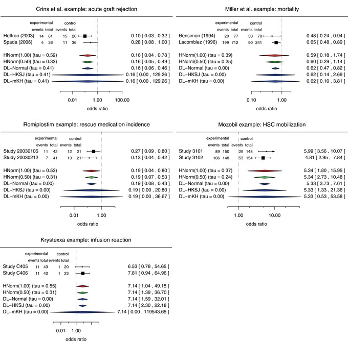
Forest plots for the five examples from rare diseases with various estimates of the treatment effect. In each panel, the top two rows show the data (numbers of cases and events in experimental and control groups) and the odds ratios with their 95% confidence intervals. The following rows show the different combined odds ratios and the estimated heterogeneity (posterior medians for the Bayesian approach).

Both studies yielded statistically significant results. However, there were some differences in the estimated odds ratios resulting in moderate to substantial estimates of the between‐trial standard deviation. Although the two studies were statistically significant, the HKSJ and mKH methods result in confidence intervals that include the null hypothesis and are extremely wide (0–129 on the odds ratio scale). In contrast, the other three meta‐analyses yield statistically significant results with the standard method based on normal quantiles giving the shortest confidence interval.

3.3. Cochrane review of Riluzole in ALS (Miller et al., 2012)

A Cochrane Review of Riluzole for amyotrophic lateral sclerosis (ALS) combined two randomized, placebo controlled, double‐blind trials (Bensimon et al., 1994; Lacomblez et al., 1996) with information on 12‐month mortality in a meta‐analysis (Miller et al., 2012). Miller et al. combined the three active doses of the dose‐ranging study by Lacomblez et al. (1996) into one group for the purpose of the presented analysis. Whereas they used relative risks for their analyses, we present here the results in terms of odds ratios (Fig. 1).

As with the previous example both studies demonstrated statistically significant effects of the experimental drug over control (see Fig. 1). While in the previous example the DL estimate of the between‐trial heterogeneity was positive, here it is zero. In comparison to Crins et al. (2014) example, here the HKSJ and the mKH methods are more informative as they are not quite as long. However, they are still considerably longer than the Bayesian intervals, which appear to be conservative since they include odds ratios of 1 although the confidence intervals of the individual studies both exclude 1.

3.4. FDA approval in orphan disease: Romiplostim

Romiplostim (Chen et al., 2007) was approved to treat Idiopathic Thrombocytopenic Purpura based on two 2:1 randomized studies. The two studies, 20030105 and 20030212, enrolled splenectomized and nonsplenectomized patients, respectively, but were similar in their designs.

Here, we focus on patients requiring rescue medications (a secondary endpoint). Both studies showed statistically significant odds ratios (ORs): 0.27 (0.09, 0.80) for 20030105 and 0.13 (0.04, 0.42) for 20030212 (Fig. 1). The ratio of ORs is 2.12, suggesting that between‐trial heterogeneity should be considered. However, the frequentist estimate $\widehat{\tau }$ is zero, resulting in a narrow confidence interval for μ. On the other hand, the HKSJ and mKN intervals are very wide and do not allow sensible conclusions about the treatment effect. The respective Bayesian intervals are much more plausible. Additionally, for both Bayesian analyses, the posterior medians (means) for τ are smaller than the respective prior medians (means), indicating that the two half‐normal priors do not unduly favor small homogeneity.

3.5. FDA approval in orphan disease: Mozobil

Mozobil (Yuan et al., 2008) was approved for the mobilization of hematopoietic stem cells in patients with lymphoma and multiple myeloma. The two 1:1 randomized studies were conducted in two different indications: 3101 in Non‐Hodgkin's Lymphoma, and 3102 in Multiple Myeloma. However, no differential treatment effect with respect to the primary endpoint was expected, which justifies a meta‐analysis of the two studies.

Both studies show statistically significant odds ratios (Fig. 1). The ratio of the odds ratios is 1.25, suggesting possibly small between‐trial heterogeneity. Unsurprisingly, the frequentist estimate $\widehat{\tau }$ is zero. The HKSJ and mKH methods again provide very wide (but fairly different) CIs: the HKSJ method leads to a conclusive result, whereas the more conservative mKH does not; this is clearly implausible, since both studies showed highly significant results. The respective Bayesian intervals are much narrower, suggesting a sensible compromise between the rather extreme (narrow and wide) frequentist counterparts.

3.6. FDA approval in orphan disease: Krystexxa

For Krystexxa (Davi et al., 2010), two 2:2:1 randomized studies were used for approval. Here, we consider only one of two treatment arms (approved dose of 8 mg every 2 weeks) and analyze a safety endpoint (infusion reaction). The two studies showed the following ORs: 6.55 (0.78, 54.60) for C405 and 7.77 (0.94, 64.72) for C406 (Fig. 1), which suggest an increase in infusion reaction.

In this example, the HKSJ and mKH intervals, which are usually very wide, give completely different answers. The HKSJ interval is even narrower than the interval based on normal approximations, whereas the mKH interval is unrealistically wide. The overly narrow HKSJ interval is due to the similar log‐odds‐ratios $y_j$ (1.88 and 2.05), which lead to a very small estimate ${\stackrel{\sim }{\sigma }}_{\mu }=0.089$ in Eq. (9); the classical estimate ${\widehat{\sigma }}_{\mu }=0.765$, which is used for mKH, is dramatically larger.

3.7. Sensitivity analyses and concluding remarks on the applications

In this section, we presented five examples from a range of rare diseases. In each of these, two studies were combined in meta‐analyses in situations where between‐study heterogeneity had to be suspected. Still the DL estimator for the between‐study heterogeneity was zero in four out of the five examples. Furthermore, the standard approach based on normal quantiles led to the shortest intervals in all but the Krystexxa example, in which the HKSJ interval was very narrow. Otherwise the HKSJ and mKH methods yielded overall long to extremely long confidence intervals not conveying useful information on the size of the treatment effect. This is not surprising, since the 97.5% quantile of a t‐distribution with 1 degree of freedom is about 12.7. Although the Bayesian intervals appeared to be conservative, they led to interpretable results and a sensible compromise between the very short intervals based on normal quantiles and the often extremely long intervals based on t‐quantiles.

To assess the robustness of Bayesian conclusions for the five applications, log‐normal priors for τ and Gamma priors for the precision ${\tau }^{-2}$ were considered. To reflect the two scenarios with weak information, small to large and small to very large heterogeneity, the prior parameters were chosen such that prior 90%‐intervals are equal to the ones from the HN(0.5) and HN(1.0) priors.

Figure 2 shows the three types of priors for the two heterogeneity scenarios. The half‐normal priors spread their probability mass in the critical regions more evenly and are therefore recommended. Of course, if solid prior information about heterogeneity is available, the prior should be chosen accordingly.

Figure 2.

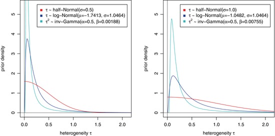
Densities of priors for the between‐trial heterogeneity used in the sensitivity analyses. The parameters for the log‐normal and inverse‐Gamma distributions were chosen so that the 5% and 95% quantiles match with those of the corresponding half‐normal distributions, that is HN(0.5) and HN(1.0) in the left and right panel, respectively.

Table 2 shows posterior medians and 95%‐intervals for the combined odds ratio $exp(\mu )$ (see also figures in supplementary material). While the different prior distributions are to some degree reflected in the posteriors (with more prior probability concentrated near zero leading to narrower intervals, as is the case with the inverse‐Gamma prior), results for μ are quite consistent and considerably more robust than the ones for the various frequentist methods.

Table 2.

Effect estimates (posterior medians and 95% credibility intervals) for the examples from Section 3 using different priors for the heterogeneity τ

Heterogeneity prior	Crins et al.	Miller et al.	Mozobil	Romiplostim	Krystexxa
$\tau \sim \phantom{}$half‐Normal(1.0)	0.16 (0.04, 0.78)	0.59 (0.18, 1.74)	5.34 (1.80, 15.95)	0.19 (0.04, 0.80)	7.14 (1.04, 49.15)
$\tau \sim \phantom{}$half‐Normal(0.5)	0.16 (0.05, 0.49)	0.60 (0.29, 1.14)	5.34 (2.73, 10.48)	0.19 (0.07, 0.53)	7.14 (1.39, 36.70)
$\tau \sim \phantom{}$log‐Normal(‐1.048,1.046)	0.16 (0.05, 0.58)	0.60 (0.27, 1.23)	5.34 (2.56, 11.19)	0.19 (0.06, 0.60)	7.14 (1.25, 40.80)
$\tau \sim \phantom{}$log‐Normal(‐1.741,1.046)	0.16 (0.06, 0.45)	0.60 (0.35, 0.99)	5.34 (3.18, 8.98)	0.19 (0.07, 0.49)	7.14 (1.46, 35.01)
${\tau }^2\sim \phantom{}$inv‐Gamma(0.5,0.0076)	0.16 (0.06, 0.47)	0.60 (0.35, 1.00)	5.34 (3.14, 9.08)	0.19 (0.07, 0.51)	7.14 (1.39, 36.57)
${\tau }^2\sim \phantom{}$inv‐Gamma(0.5,0.0019)	0.16 (0.06, 0.42)	0.61 (0.41, 0.90)	5.33 (3.45, 8.25)	0.19 (0.08, 0.46)	7.14 (1.49, 34.08)

In our investigations, we focused on the (log) odds ratio as effect measure. However, some authors prefer the relative risk over the odds ratio for the ease of interpretation. In fact, Crins et al. (2014) and Miller et al. (2012) used relative risks in their studies, presented as examples in Section 3. For these examples the conclusions did not change by using the odds ratio as effect measure instead of the relative risk.

4. Simulation study

4.1. Setup

For the simulation study of this section, we used the NNHM of Section 2. The study sample sizes n ₁ and n ₂ were set to 25, 100, or 400, which leads to six different combinations of $(n_1,n_2)$. In the following Figs. 2–4, the first rows show results for equally sized studies, while the second rows illustrate the imbalanced settings. Standard errors for the estimated log‐odds‐ratios $Y_j$ were set to $2/\sqrt{n_1}$ and $2/\sqrt{n_2}$. Without loss of generality, μ was set to zero. In terms of the “relative” amount of heterogeneity I ² (Higgins and Thompson, 2002), the different settings correspond to $I^2\in [0.20,0.80]$ for $\tau =0.2$, and to $I^2\in [0.86,0.99]$ for $\tau =1.0$. The number of simulations, which were performed using $\mathsf{R}$, was 15, 000. Simulation results are shown for the bias of τ estimates, the fraction of τ estimates equal to zero, the coverage probabilities and the interval lengths for μ.

Figure 4.

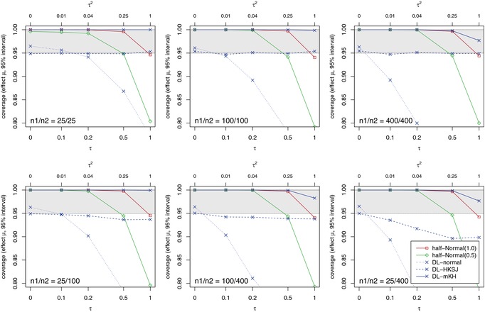
Coverage of interval estimators for different study sizes n ₁ and n ₂.

4.2. Bias in estimators of the between‐study heterogeneity τ

Figure 3 shows the bias of τ estimates. If heterogeneity is small ($\tau =0,0.1$), the DL estimator tends to overestimate τ, although this bias is generally small in comparison with other estimators. On the other hand, τ will be underestimated for substantial ($\tau =0.5$) and large ($\tau =1.0$) heterogeneity. The Bayesian estimators (posterior medians) show similar patterns, with the magnitude of bias depending on the prior. The overestimation under small heterogeneity is obviously more pronounced for the HN(1.0) than for the HN(0.5) prior, because the former favors larger values of τ. On the other hand, underestimation of τ only occurs (and is fairly small) if heterogeneity is substantial to large. It should be noted that, in contrast to the frequentist methods, the Bayesian estimates for τ are less important, since the inference for μ takes into account the uncertainty of τ via the posterior distribution.

Figure 3.

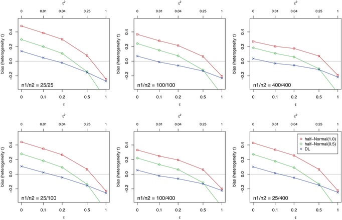
Bias in estimating the between‐study heterogeneity τ for different study sizes n ₁ and n ₂.

4.3. Fraction of zero τ estimates

Table 3 shows that the DL estimates for τ are often zero even if heterogeneity is substantial $(\tau =0.5)$ or large $(\tau =1.0)$. This is a well‐known problem, which, if not appropriately addressed, results in too optimistic inferences for μ.

Table 3.

Fractions (in %) of heterogeneity estimates turning out as zero

	True heterogeneity τ
$n_1/n_2$	0.0	0.1	0.2	0.5	1.0
25/25	68	67	62	47	29
100/100	68	63	52	29	15
400/400	68	53	34	16	8
25/100	68	65	60	41	23
100/400	68	61	46	24	13
25/400	68	65	59	39	22

4.4. Coverage probabilities and interval lengths for μ

As can be seen from Fig. 4, if heterogeneity is small, all methods work well save for the normal approximation (DL‐normal), for which the coverage can be below the nominal level even for small heterogeneity $(\tau =0.1)$. The HKSJ method is known to work well for equally sized studies, but can be problematic for unequal study sizes and considerable heterogeneity. As can be seen, the modified method (mKH) resolves this problem. The Bayesian intervals show good coverage in the range of the prior, irrespective of the study sizes. For example, under the more optimistic HN(0.5) prior, coverage is reasonable for τ up to substantial heterogeneity ($\tau =0.5$), but will drop considerably for larger values that are a‐priori less likely.

Coverage is obviously linked to interval length: higher coverage generally comes at the price of longer intervals. Figure 5 shows that this price can be very high. The two frequentist methods with good coverage (HKSJ, mKH) exhibit exorbitantly long and implausible 95%‐intervals, for which practical relevance is unclear. Interestingly, the Bayesian intervals (for all priors considered; see also supplementary material) are much shorter and provide a sensible compromise between the HKSJ or mKH and the DL‐normal intervals. These findings are consistent with results of the examples in Section 3.

Figure 5.

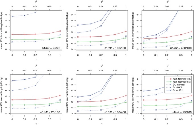
Mean lengths of confidence and credibility intervals for different study sizes n ₁ and n ₂.

5. Discussion

There is a need for random‐effects meta‐analyses with only two studies, in particular in rare diseases. To gain insights into the properties of various meta‐analytic methods for two trials, in this special case we considered examples from the area of rare diseases and conducted an extensive simulation study. The simulations allowed us to assess the coverage probabilities and mean lengths of the confidence and credibility intervals. The examples led to further insights into the interpretability of results.

We can summarize our findings as follows. The confidence intervals based on normal quantiles do not have the right coverage and cannot be recommended for use in the case of two studies. The HKSJ intervals provide good coverage if the standard errors of the treatment effects observed in the two studies are of similar size. In general, however, the HKSJ intervals are either so wide that they do not allow any conclusion, or are very narrow. The latter occurs rarely (if the two study estimates are very close, (9)), but can lead to problematically narrow confidence intervals and unfavorable coverage. This can be fixed by the ad‐hoc modification (mKH), which is in agreement with findings by Röver et al. (2015). The mKH method yields generally coverage probabilities in excess of the nominal level, but the intervals are generally so wide that they do not allow any meaningful conclusion. In this sense, we agree with Gonnermann et al. (2015) that there is currently no solution for random‐effects meta‐analysis in the frequentist setting. However, Bayesian random‐effects meta‐analyses with a reasonable prior yield interpretable results in our examples and showed satisfying properties in the simulations. Therefore, the Bayesian intervals appear to be a reasonable compromise between the extremes of the confidence intervals based on normal quantiles that suffer from poor coverage and the t‐distribution based intervals that tend to be so long that they are inconclusive.

Use of a Bayesian approach of course entails the question of what constitutes sensible prior information in a given context. This may be argued on the basis of the endpoint in question, that is, what is the plausible amount of heterogeneity expected, for example among log‐ORs, as in the motivating examples above. In such situations we recommend following the arguments given by Spiegelhalter et al. (2004, Section 5.7.3) and using weakly informative half‐normal priors, which lead to reasonable results here. Otherwise the problem may be to determine what constitutes relevant external data, and how this information may be utilized to formulate a prior, as was done, for example by Turner et al. (2012) and Rhodes et al. (2015).

Here we investigated several meta‐analytic methods for two studies, with a focus on rare diseases. While a definite answer to this challenging problem is under dispute, the proposed Bayesian approach works well in our examples and simulation settings. The current frequentist methods have severe limitations, which may be addressed with future research. Until these limitations are resolved, we recommend to meta‐analyze two heterogeneous studies in a Bayesian way using plausible priors.

Conflict of interest

B.N. and S.W. are employees of Novartis, the manufacturer of an interleukin‐2 receptor antagonist used in the example of Section 3.2.

Supporting information

Supporting Information

Supporting Information

References

- Bensimon, G. , Lacomblez, L. , Meininger, V. and the ALS/Riluzole Study Group (1994). A controlled trial of Riluzole in amyotrophic lateral sclerosis. The New England Journal of Medicine 330, 585–591. [DOI] [PubMed] [Google Scholar]
- Chen, Y. W. , Zalkikar, J. , Chakravarty, A. , Jamali, F. , Robie‐Suh, K. , Rieves, R. and Moore, F. (2007). Nplate (Romiplostim). Statistical Review and Evaluation BB 125168/0, U.S. Department of Health and Human Services, Food and Drug Administration (FDA).
- Crins, N. D. , Röver, C. , Goralczyk, A. D. and Friede, T. (2014). Interleukin‐2 receptor antagonists for pediatric liver transplant recipients: a systematic review and meta‐analysis of controlled studies. Pediatric Transplantation 18, 839–850. [DOI] [PubMed] [Google Scholar]
- Davey, J. , Turner, R. M. , Clarke, M. J. and Higgins, J. P. (2011). Characteristics of meta‐analyses and their component studies in the Cochrane Database of Systematic Reviews: a cross‐sectional, descriptive analysis. BMC Medical Research Methodology 11, 160. [DOI] [PMC free article] [PubMed] [Google Scholar]
- Davi, R. C. , Buenconsejo, J. , Hull, K. , Okada, S. and Sista, R. (2010). KrystexxaTM (Pegloticase, PEG‐uricase and Puricase). Statistical Review and Evaluation STN 125293‐0037, U.S. Department of Health and Human Services, Food and Drug Administration (FDA).
- DerSimonian, R. and Kacker, R. (2007). Random‐effects model for meta‐analysis of clinical trials: an update. Contemporary Clinical Trials 28, 105–114. [DOI] [PubMed] [Google Scholar]
- DerSimonian, R. and Laird, N. (1986). Meta‐analysis in clinical trials. Controlled Clinical Trials 7, 177–188. [DOI] [PubMed] [Google Scholar]
- Dias, S. , Sutton, A. J. , Welton, N. J. and Ades, A. E. (2012). Heterogeneity: subgroups, meta‐regression, bias and bias‐adjustment. NICE DSU Technical Support Document 3, National Institute for Health and Clinical Excellence (NICE). [PubMed]
- Dias, S. , Sutton, A. J. , Welton, N. J. and Ades, A. E. (2014). A generalized linear modelling framework for pairwise and network meta‐analysis of randomized controlled trials. NICE DSU Technical Support Document 2, National Institute for Health and Clinical Excellence (NICE). [PubMed]
- European Medicines Agency (EMEA) (1998). Note for guidance on statistical principles for clinical trials. CPMP/ICH/363/96.
- European Medicines Agency (EMEA) (2001). Points to consider on application with 1. meta‐analyses; 2. one pivotal study. CPMP/EWP/2330/99.
- Follmann, D. A. and Proschan, M. A. (1999). Valid inference in random effects meta‐analysis. Biometrics 55, 732–737. [DOI] [PubMed] [Google Scholar]
- Friede, T. , Röver, C. , Wandel, S. and Neuenschwander, B. (2016). Meta‐analysis of few small studies in orphan diseases Research Synthesis Methods. DOI: 10.1002/jrsm.1217. [DOI] [PMC free article] [PubMed] [Google Scholar]
- Gonnermann, A. , Framke, T. , Großhennig, A. and Koch, A. (2015). No solution yet for combining two independent studies in the presence of heterogeneity. Statistics in Medicine 34, 2476–2480. [DOI] [PMC free article] [PubMed] [Google Scholar]
- Hartung, J. and Knapp, G. (2001a). On tests of the overall treatment effect in meta‐analysis with normally distributed responses. Statistics in Medicine 20, 1771–1782. [DOI] [PubMed] [Google Scholar]
- Hartung, J. and Knapp, G. (2001b). A refined method for the meta‐analysis of controlled clinical trials with binary outcome. Statistics in Medicine 20, 3875–3889. [DOI] [PubMed] [Google Scholar]
- Hedges, L. V. and Olkin, I. (1985). Statistical Methods for Meta‐Analysis. Academic Press, San Diego, CA, USA. [Google Scholar]
- Heffron, T. , Pillen, T. , Smallwood, G. , Welch, D. , Oakley, B. and Romero, R. (2003). Pediatric liver transplantation with Daclizumab induction. Transplantation 75, 2040–2043. [DOI] [PubMed] [Google Scholar]
- Higgins, J. P. T. and Thompson, S. G. (2002). Quantifying heterogeneity in a meta‐analysis. Statistics in Medicine 21, 1539–1558. [DOI] [PubMed] [Google Scholar]
- International Conference on Harmonisation of Technical Requirements for Registration of Pharmaceuticals for Human Use (ICH) (2002). The common technical document for the registration of pharmaceuticals for human use. Efficacy M4E(R1).
- Knapp, G. and Hartung, J. (2003). Improved tests for a random effects meta‐regression with a single covariate. Statistics in Medicine 22, 2693–2710. [DOI] [PubMed] [Google Scholar]
- Lacomblez, L. , Bensimon, G. , Meininger, V. , Leigh, P. , Guillet, P. and Amyotrophic Lateral Sclerosis/Riluzole Study Group II , (1996). Dose‐ranging study of riluzole in amyotrophic lateral sclerosis. Lancet 347, 1425–1431. [DOI] [PubMed] [Google Scholar]
- Miller, R. , Mitchell, J. and Moore, D. (2012). Riluzole for amyotrophic lateral sclerosis (als)/motor neuron disease (mnd). Cochrane Database of Systematic Reviews 3, CD001447. [Google Scholar]
- Neuenschwander, B. , Capkun‐Niggli, G. , Branson, M. and Spiegelhalter, D. J. (2010). Summarizing historical information on controls in clinical trials. Clinical Trials 7, 5–18. [DOI] [PubMed] [Google Scholar]
- Rhodes, K. M. , Turner, R. M. and Higgins, J. P. T. (2015). Predictive distributions were developed for the extent of heterogeneity in meta‐analyses of continuous outcome data. Journal of Clinical Epidemiology 68, 52–60. [DOI] [PMC free article] [PubMed] [Google Scholar]
- Röver, C. , Knapp, G. and Friede, T. (2015). Hartung‐Knapp‐Sidik‐Jonkman approach and its modification for random‐effects meta‐analysis with few studies. BMC Medical Research Methodology 15, 99. [DOI] [PMC free article] [PubMed] [Google Scholar]
- Rukhin, A. L. (2012). Estimating common mean and heterogeneity variance in two study case meta‐analysis. Statistics and Probability Letters 82, 1318–1325. [Google Scholar]
- Schmidli, H. , Gsteiger, S. , Roychoudhury, S. , O'Hagan, A. , Spiegelhalter, D. and Neuenschwander, B. (2014). Robust meta‐analytic‐predictive priors in clinical trials with historical control information. Biometrics 70, 1023–1032. [DOI] [PubMed] [Google Scholar]
- Sidik, K. and Jonkman, J. N. (2003). On constructing confidence intervals for a standardized mean difference in meta‐analysis. Communications in Statistics Simulation and Computation 32, 1191–1203. [Google Scholar]
- Spada, M. , Petz, W. , Bertani, A. , Riva, S. , Sonzogni, A. , Giovanelli, M. , Torri, E. , Torre, G. , Colledan, M. and Gridelli, B. (2006). Randomized trial of Basiliximab induction versus steroid therapy in pediatric liver allograft recipients under tacrolimus immunosuppression. American Journal of Transplantation 6, 1913–1921. [DOI] [PubMed] [Google Scholar]
- Spiegelhalter, D. J. , Abrams, K. R. and Myles, J. P. (2004). Bayesian Approaches to Clinical Trials and Health‐care Evaluation. New York, NY: Wiley & Sons, Chichester, UK. [Google Scholar]
- Turner, R. M. , Davey, J. , Clarke, M. J. , Thompson, S. G. and Higgins, J. P. T. (2012). Predicting the extent of heterogeneity in meta‐analysis, using empirical data from the Cochrane Database of Systematic Reviews. International Journal of Epidemiology 41, 818–827. [DOI] [PMC free article] [PubMed] [Google Scholar]
- Turner, R. M. , Jackson, D. , Wei, Y. , Thompson, S. G. and Higgins, P. T. (2015). Predictive distributions for between‐study heterogeneity and simple methods for their application in Bayesian meta‐analysis. Statistics in Medicine 34, 984–998. [DOI] [PMC free article] [PubMed] [Google Scholar]
- Veroniki, A. A. , Jackson, D. , Viechtbauer, W. , Bender, R. , Bowden, J. , Knapp, G. , Kuß, O. , Higgins, J. P. T. , Langan, D. and Salanti, G. (2016). Methods to estimate the between‐study variance and its uncertainty in meta‐analysis. Research Synthesis Methods 7, 55–79. [DOI] [PMC free article] [PubMed] [Google Scholar]
- Yuan, W. , He, K. , Sridhara, R. , Brave, M. , Justice, R. and Jenney, S. (2008). MozobilTM (Plerixafor injection). Statistical Review and Evaluation 22,311/000, U.S. Department of Health and Human Services, Food and Drug Administration (FDA).
Associated Data
This section collects any data citations, data availability statements, or supplementary materials included in this article.
Supplementary Materials