Factors affecting characterization and localization of interindividual differences in functional connectivity using MRI

Abstract

Much recent attention has been paid to quantifying anatomic and functional neuroimaging on the individual subject level. For optimal individual subject characterization, specific acquisition and analysis features need to be identified that maximize interindividual variability while concomitantly minimizing intra‐subject variability. We delineate the effect of various acquisition parameters (length of acquisition, sampling frequency) and analysis methods (time course extraction, region of interest parcellation, and thresholding of connectivity‐derived network graphs) on characterizing individual subject differentiation. We utilize a non‐parametric statistical metric that quantifies the degree to which a parameter set allows this individual subject differentiation by both maximizing interindividual variance and minimizing intra‐individual variance. We apply this metric to analysis of four publicly available test‐retest resting‐state fMRI (rs‐fMRI) data sets. We find that for the question of maximizing individual differentiation, (i) for increasing sampling, there is a relative tradeoff between increased sampling frequency and increased acquisition time; (ii) for the sizes of the interrogated data sets, only 3‐4 min of acquisition time was sufficient to maximally differentiate each subject with an algorithm that utilized no a priori information regarding subject identification; and (iii) brain regions that most contribute to this individual subject characterization lie in the default mode, attention, and executive control networks. These findings may guide optimal rs‐fMRI experiment design and may elucidate the neural bases for subject‐to‐subject differences. Hum Brain Mapp 37:1986–1997, 2016. © 2016 Wiley Periodicals, Inc.

Abbreviations

DMN

Default mode network

PCA

Principal component analysis

ROI

Region of interest

INTRODUCTION

Many neuroimaging studies seek to use interindividual variability in anatomic and functional characterization to gain insight into concomitant variability in a behavioral or clinical feature of interest [Kanai and Rees, 2011; Zilles and Amunts, 2013]. Additionally, just as a psychologist may use a patient's behavioral score to predict an outcome or guide a treatment, and just as a genomic profiling may assess genetic contribution to disease risk, there has been interest in developing methods and standards that allow for individual patient anatomic and functional characterization using neuroimaging [Atluri et al., 2013].

Recent studies have indeed identified significant interindividual variability in behavioral, anatomic and functional features, and determined that these variables correlate in significant and intriguing ways. Kanai and Rees catalogued numerous examples of studies where particular behavioral traits can be predicted by individual subject level region‐specific anatomic (DTI, VBM) or functional (BOLD fMRI, PET, MEG, EEG, MRS) measures [Mueller et al., 2013]. Additionally, Mueller et al. demonstrated that there is significant interindividual variability in functional connectivity assessed with resting state fMRI (rs‐fMRI), and that regions of high variability correlate with regions of evolutionarily recent cortical expansion as well as regions thought to determine higher cognitive function [Mueller et al., 2013]. More recently, Finn et al [2015] demonstrated that functional connectivity is unique across subjects and that it can be used to identify an individual within a large group.

For studies that seek to develop a functional characterization of an individual subject, specific acquisition and analysis features can be identified that maximize this interindividual variability while minimizing intra‐subject variability. We therefore sought to expand on the above referenced studies to analyze rs‐fMRI data for factors that affect this individual subject differentiation, given the emergence of rs‐fMRI as a powerful tool for both neuroscience and clinical application [Fornito and Bullmore, 2011; Lee et al., 2013; Snyder and Raichle, 2012]. In particular when compared to task‐based fMRI, rs‐fMRI has received interest as a clinical tool due to (i) a lack of dependence on subject compliance and performance on a particular task, (ii) a lack of need for specialized stimulus presentation hardware and software, and (iii) potentially lower cumulative acquisition times [Kelly et al., 2012]. The lack of dependence on subject compliance is particularly important in certain patient classes, such as those with functional deficits related to brain lesions; patients who may not be able to understand the task due to cognitive, hearing or visual disability; patients with language barriers; or in the pediatric population.

There are important differences between the analysis of task‐based and resting‐state fMRI data. Without a task with which to correlate, pairwise similarities between regions or voxel timecourses are computed instead of a univariate analysis of the time‐series. Additionally, a whole‐brain or network based approach is often utilized as there may be no a priori knowledge regarding regions of interest. Typically in rs‐fMRI connectivity studies, a parameter of similarity (e.g., Pearson correlation, partial correlation, spectral coherence) is calculated between pairs of timecourses from given regions of interest. These similarity data are organized into an adjacency matrix, one calculated per each subject or scan. Fundamentally each summary statistic, such as “global efficiency” [Rubinov and Sporns, 2010], calculated in a rs‐fMRI study is a calculation of the data in these adjacency matrices [Van Dijk et al., 2010].

While group‐level reproducibility of rs‐fMRI has been demonstrated for several specific ROIs and networks [Biswal et al., 2010; Chou et al., 2012; Damoiseaux et al., 2006; Song et al., 2012; Wang et al., 2013], an analysis of whole‐brain subject level variability has only recently been described [Mueller et al., 2013], as has the observation that rs‐fMRI data could be used to identify individuals [Finn et al., 2015]. Mueller et al demonstrate a relatively conserved topographic distribution of variability of functional connectivity across individuals, with this variability increased in heteromodal association cortices compared to unimodal sensorimotor regions. With a priori knowledge of a large set of connectivity matrices associated with particular subjects, Finn et al demonstrate that an individual's connectivity profile is unique enough to allow identification based on the labeled target set. Both studies utilize single test‐retest resting state‐fMRI datasets, and examine the effect of subject motion on affecting individual characterization; the latter study further examines additional contributory variables such as length of acquisition and parcellation schemes.

We extend the investigation in two significant ways: first we include data from four publicly available resting state‐fMRI test‐retest datasets which vary in acquisition parameters. The datasets include both single‐band and multiband acquisitions, allowing for inclusion of sampling frequency as a variable. Second, we develop a non‐parametric, rank‐based statistical metric that allows us to quantify the degree to which a given acquisition and analysis scheme maximizes interindividual variability while minimizing intra‐individual variability. We then use this metric to determine which factors most contribute to individual subject differentiation. A non‐parametric, rank‐based statistic has several advantages compared to more typical approaches, such as intraclass correlation [Shrout and Fleiss, 1979]. First, it can operate readily on multivariate and non‐Euclidean quantitative data. Second, it is model‐free, in that it does not make any assumptions about the distribution of the data. Third, because it is based on order statistics, it is robust to many kinds of artifacts, such as spurious or missing data.

METHODS

We examined the effect of the following variables in determining subject characterization on four different resting state fMRI datasets: length of acquisition, sampling frequency, parcellation scheme, and method of time course extraction. In addition, we determined whether nuisance variables (motion and physiological noise) contributed to individual differentiation. For differentiation, an unsupervised test‐retest pairing algorithm was used, as described below. The regions of the brain that most contribute to individual differentiation were also investigated.

Data Sets Analyzed

Four publicly available data sets were analyzed, each consisting of two resting‐state fMRI acquisitions separated in time. Each of these data sets is available publicly through the Neuroimaging Informatics Tools and Resources Clearinghouse (NITRC; http://www.nitrc.org):

1. KKI: A total of 21 subjects, ages 22–61 years, each scanned twice at 3T for 7 minutes, TR = 2.0 sec. One subject was excluded due to an artifact evident during one of the acquisitions. Scan details: single band 2D EPI ascending order; 3 mm isotropic voxels (80 × 80 voxels), TE 30 ms; flip angle 75° [Landman et al., 2011].

2. NKI Standard: A total of 23 subjects, ages 19–60 years, each scanned twice at 3T using single band sequences for 5 minutes, TR = 2.5 sec. Scan details: single band 2D EPI interleaved order; 3mm isotropic voxels (72 × 72 voxels), TE 30 ms; flip angle 80° [Nooner et al., 2012].

3. NKI Multiband: TR = 1.4 sec: Same subjects and scanner as NKI Standard, each scanned twice using a multiband sequence for 10 minutes, with TR = 1.4 sec. Scan details: multi band 2D EPI of acceleration factor 4; interleaved order; 2 mm isotropic voxels (112 × 112 voxels), TE 30 ms; flip angle 65° [Nooner et al., 2012].

4. NKI Multiband: TR = 0.645 sec: Same subjects and scanner as NKI Standard, each scanned twice using a multiband sequence for 10 minutes, with TR = 0.645 sec. Scan details: multi band 2D EPI of acceleration factor 4; interleaved order; 3mm isotropic voxels (74 × 74 voxels), TE 30 ms; flip angle 60° [Nooner et al., 2012].

Adjacency Matrix Construction

For each scan of each data set, an adjacency matrix describing its functional connectivity was constructed via the following steps.

Pre‐processing: For pre‐processing we used a series of steps common to many resting state fMRI studies (e.g., [Landman et al., 2011]), with the details of specific steps described below. Following data retrieval from the NITRC, we conducted the following pre‐processing on each scan independently. Each BOLD time‐series underwent a standard preprocessing sequence of slice timing correction, motion correction/realignment, co‐registration to the subject's anatomic T1‐weighted images, spatial normalization to the Montreal Neurological Institute MNI152 2mm template using ANTs (Advanced Normalization Tools) registration (stnava.github.io/ANTs), detrending via high pass filtering, principal component analysis (PCA)‐based CSF and white matter nuisance regression (following [Behzadi et al., 2007]), 6 parameter motion regression, bandpass temporal filtering (0.01–0.1 Hz), and spatial smoothing (6mm Gaussian kernel). For PCA‐based nuisance regression, anatomic CSF and white matter masks were generated from segmentation maps that were then eroded by one (CSF) or two (white matter) voxels. Nuisance regressors were estimated as PCA components that encompass up to 95% of the variance of the unsmoothed time‐series corresponding to each of the eroded masks. Spatial smoothing was completed as it may improve signal to noise, allow for a more Gaussian distribution of the series data, and is a standard preprocessing routine for many rs‐fMRI studies. Note that the multiband data sets did not undergo slice‐timing correction. All analysis was completed in MATLAB (Mathworks, Natick, MA) and SPM8 (Wellcome Trust, UK). We specifically chose not to apply global signal regression as recent studies have suggested that this step may exacerbate motion related artifacts [Jo et al., 2013] and that global rs‐fMRI signal may have significant neurophysiological correlates of interest [Schölvinck et al., 2010].

Parcellation Scheme: After preprocessing, a parcellation map was applied to the time‐series data so that each gray matter voxel was uniquely assigned to one region of interest (ROI). Two parcellation schemes were tested. For each, the target number of regions of interest (ROIs) for each parcellation scheme was varied in powers of 2 from 128 to 2048. The highest target number of 2048 was chosen as at this target the typical ROI size was slightly larger than the Gaussian kernel used for spatial smoothing in preprocessing, thereby allowing the highest ROI number that maintained minimal ROI interdependence.

For the first parcellation scheme, the “uniform” type, the gray matter was subdivided into uniform sized ROIs (maximum of size differences between ROIs was one voxel) using the algorithm of Zalesky et al. [2010].

For the second scheme, the “functional” type, we utilized a scheme from Craddock et al. based on clustering rs‐fMRI data [Craddock et al., 2012]. The goal of this method was to cluster voxels with the highest effective intra‐ROI connectivity versus inter‐ROI connectivity, while maintaining spatial proximity [Craddock et al., 2012]. Of note, due to the clustering algorithm the number of ROIs in the resultant parcellation may be lower than the indicated target ROI number, especially for larger target ROI numbers. In accord with the published protocol for this scheme, the fMRI data used for generating these parcellations were from three subjects from a different, publicly available data set included in the distribution of the published parcellation code.

After calculating a parcellation for each of the above target ROI values, via either of the above schemes, the same set of parcellations was used throughout the analyses described below.

Timecourse Extraction and Adjacency Matrix Construction: Timecourses were extracted from each ROI as either the average (mean) of the timecourses corresponding to each voxel, or the first principal component (eigenvariate) of the collection of ROI timecourses.

Following timecourse extraction, an “adjacency matrix” was calculated in which each matrix row and column corresponded to a single ROI, and matrix elements corresponded to Pearson correlation coefficients between the pair of timecourses for the ROIs of that row and column. In other words, a weighted non‐directional graph was calculated for each dataset with graph vertices corresponding to each parcellation ROI and graph edge weight (w) calculated as the Pearson correlation coefficient (w = r) between the timecourses of the corresponding ROI pair.

As rs‐fMRI analysis can be significantly affected by noise, we aimed to evaluate the degree to which nuisance timecourse correlations influenced our results. For this nuisance‐based analysis (Fig. 3, third and fourth rows), pairwise Pearson correlation coefficients between nuisance regressor timecourses were used for each scan to generate the initial adjacency matrix edge weights, instead of the denoised ROI timecourses.

Figure 3.

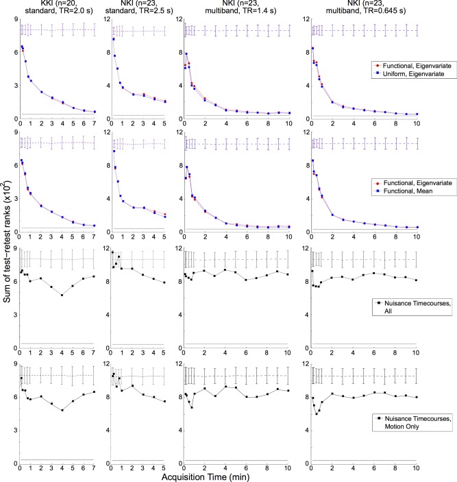
Varying methods of time‐series extraction and parcellation generation for each test‐retest data set and analysis of nuisance timecourses. First row: Sum of test‐retest scan pairs comparing method of timecourse‐series extraction, plotted similar to Figure 2. See “Methods” section for details. Second row: Sum of test‐retest scan pairs comparing method of parcellation generation, plotted similar to Figure 2. Third row: Sum of test‐retest scan pairs for adjacency matrices calculated from the nuisance timecourses (motion, CSF, white matter, and global signal), plotted similar to Figure 2. Fourth row: Sum of test‐retest scan pairs for adjacency matrices calculated from the motion‐related nuisance time‐ courses only, plotted similar to Figure 2. [Color figure can be viewed in the online issue, which is available at http://wileyonlinelibrary.com.]

Thresholding: In the case of thresholded analysis (Fig. 4), edge weights lower than an indicated percentile threshold across the graph were set to zero.

Figure 4.

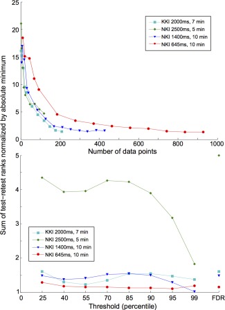
Factors affecting achieving the minimum rank sum. Top: Rank sums of test‐retest pairs for each data set as a function of number of data points acquired. Bottom: Adjacency matrices were thresholded such that edges with correlation less than the indicated percentile were set to zero (FDR: threshold set to the Benjamini‐Hochberg false discovery rate). Values presented are for the indicated data set processed using the functional parcellation of 1920 ROIs and using eigenvariate time‐series extraction. [Color figure can be viewed in the online issue, which is available at http://wileyonlinelibrary.com.]

Individual Differentiation Efficacy

Rank sum statistic

We developed a metric that would allow us to quantify the efficacy and efficiency of the choice of analysis procedure to differentiate individuals (Fig. 1).

Figure 1.

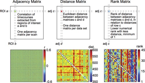
Minimum rank sum statistic enables non‐parametric comparisons of test‐retest acquisition and analysis parameters. To assess the efficacy of differentiating individual subjects, adjacency matrices were first made for each scan where each matrix element corresponded to the correlation between time‐series extracted from the indicated pair of regions of interest (ROIs; left, schematic on top, example from real data on bottom). The adjacency matrix shown here represents a sample correlation matrix of a subject using a parcellation generated with a target of 2048 ROIs; additional adjacency matrices for each parcellation were created as described in the methods. Each row or column therefore corresponds to one ROI. Next, for each dataset a distance matrix was calculated where each element corresponded to the Euclidean distance (square root of sum of square differences for individual matrix elements) between the indicated pair of adjacency matrices (middle). Thus, for the KKI dataset, each matrix element represents the distance between two adjacency matrices of the 40 individual scans (20 individual subjects × 2 scans each), and for each NKI dataset, each element represents the distance between two adjacency matrices of the 46 individual scans (23 individual subjects × 2 scans each). The sample matrix shown here represents a distance matrix utilizing the NKI Standard dataset. Each row or column therefore corresponds to one scan. Then, a rank matrix was calculated where each element corresponds to the rank of the distance between the indicated pair of scans compared to the set of distances in that row. The sample matrix shown here represents a rank matrix utilizing the NKI Standard dataset. Note, the rank matrix is not necessarily symmetric (right; minimum rank equals 1). [Color figure can be viewed in the online issue, which is available at http://wileyonlinelibrary.com.]

We consider a non‐parametric, order based strategy. To proceed, we first calculated a distance matrix d_{k , k ′} = δ(G_k, G _k ′) for graphs G_k and G _k ′. In our current analysis, δ(G_k,G _k ′) =  $\sqrt{{\sum }_{ij}{(w_{ij}‐{w^{\text{'}}}_{ij})}^2}$ where w_ij, w'_ij are edge weights between the ith and jth ROIs of graphs G_k, G _k ′ respectively.

Then, from the distance matrix, we calculated a rank matrix as follows: for the ith row (which corresponds to the ith scan) in the distance matrix, a numerical rank between 0,1,2,…n − 1, is assigned to each element, where n is the number of scans in the data set, and so that a rank of 0 is assigned to the element corresponding to the distance between a the graph of a scan and itself, and a rank of n − 1 corresponds to the maximal distance between pairs of adjacency matrices in that row.

The rank sum metric is the sum of these numerical ranks across all the elements of the rank matrix that correspond to true test and retest scan pairs, e.g., the first off‐diagonal elements of a rank matrix in which true test and retest pairs are in adjacent rows/columns. Ideally, the distance between the graphs of true test‐retest pairs will be the smallest nonzero distance, so that these ranks will be 1 across the data set. Correspondingly, the ideal rank sum would be equal to n, the number of scans in the data set. The minimum rank sum is the ideal sum of n, and the maximum rank sum is n(n − 1) so that this metric is closed and bounded, with a range that is independent of the choice or scale of the particular distance metric. We can therefore grade the ability of an analysis procedure to differentiate individuals within a test‐retest data set by how closely its rank sum approximates n.

The benefits of using this statistic for comparison include having an absolute minimum (equal to the number of scans in the data set) and easy to define statistics based on random permutation of pairings. This metric is minimized by factors that allow maximal differentiation of individual subjects, with greatest reproducibility (minimal inter‐individual variance) between test and retest.

Permutation testing

To generate a distribution that the calculated rank sums could be compared to, 1,000 rank sums were calculated using random pairings of scans across the data set, without including the true test‐retest pairings. Notably, the true pairing is only one of n!/[2*(n/2)!] possible pairing that these 1,000 permutations sample from, where n is the number of scans in the data set.

Unsupervised sorting of test‐retest pairs

An unsupervised genetic algorithm, one in which no a priori knowledge of subject labeling was included, was developed to find the pairings of scans within each data set that minimized the rank sum, under the hypothesis that such a search would find the true test‐retest pairings as those pairs should have minimal differences between their adjacency matrices and therefore minimal total rank sum. The genetic algorithm optimization was completed using the “gaoptimset” function of MATLAB.

A population of random pairings of scan numbers was generated, with each pairing represented as a string of numbers corresponding to the scan IDs taken as pairs.

The crossover function of the optimization generated members of a subsequent population by flipping the ordering of a substring of the string of the prior generation.

The mutation function of the optimization generated members of a subsequent generation by swapping random elements of the string of the prior generation.

Finally the fitness function was minimization of the rank sum for each member of the population, which was computed using the corresponding distance matrices (see Fig. 1).

Each generation consisted of a population of 100 strings and each optimization was run for 400,000 generations, with convergence halted if the average change over successive generations was less than the internal default tolerance function.

Each optimization was repeated for subsamplings of acquisition time of length 9, 15, 30, and 45 seconds, and 1 min, 2 min, 3 min and so on up to the maximum acquisition time for that data set. Presented are the minimal acquisition times for generating perfectly accurate test‐retest pairings for the indicated condition.

Localization of Interindividual Differences

To determine the brain regions and connections that contribute to this individual subject differentiation, for each dataset the rank sum metric was calculated for differences of each element of the adjacency matrix (using the functional parcellation, with the maximal number of ROIs, and eigenvariate time‐series extraction). The brain regions containing the highest proportion of edges with the lowest rank sum (< 5^th percentile across all edges) were determined (Fig. 5). To determine the relevant networks represented by these ROIs, large scale resting state networks were identified by performing K means clustering with target k = 10 on an adjacency matrix averaged across all subjects and datasets, utilizing the 1,000 ROI functional parcellation. The resultant 10 clusters were manually labeled as one of the known canonical resting state networks based on the topographic features of the clusters.

Figure 5.

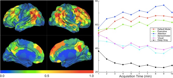
Map of brain regions that define unique identifiers of individuals. Left: Brain regions color coded by greatest proportion of connections with the lowest (< 5^th percentile) test‐retest rank sum, averaged across the four data sets, calculated using all the available acquisition time. Similar results were found for each individual data set (Supporting Information Fig. S1). Warmer colors code to regions that enable higher individual differentiation (higher number of connections that have low test‐retest rank sum). Right: Average number of low (<5^th percentile) rank sum edges per ROI for the indicated resting state network, averaged across the data sets at the indicated amounts of acquisition time. For data sets with <10 min of acquisition time, KKI and NKI 2500, their adjacency matrices using the full amount of acquisition time (7 min for KKI, 5 min for NKI 2500) were used in the average for the later time points. [Color figure can be viewed in the online issue, which is available at http://wileyonlinelibrary.com.]

RESULTS

Maximizing Ability to Differentiate Individuals

We used minimization of the rank sum statistic (described in Methods) to define the ability of a method to differentiate individual subjects. For each analysis and acquisition parameter that was varied, several general trends were seen (Figs. 2 and 3). As expected, a longer acquisition time and a higher number of ROIs in the parcellation allowed greater ability to differentiate between individual subjects, with acquisition parameters (such as length of acquisition and TR) having greater effect.

Figure 2.

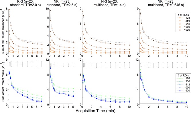
Varying acquisition time and parcellation for each test‐retest data set. Top: Sum of distances (a measure of intra‐individual reproducibility; lower distances imply lower variability and higher reproducibility) between test‐retest scan pairs versus acquisition time, for varied number of regions of interest in each parcellation (data using a functional parcellation scheme [Craddock RC et al., 2012] and eigenvariate time extraction; see “Methods” section: Methods for details). Dashed line is the mean ± s.e.m. calculation for a set of 1000 randomly assorted pairs for the maximum ROI parcellation. Bottom: Sum of ranks of test‐retest scan pairs (a measure of interindividual differentiability; lower sums indicate higher individual differentiability) for the indicated data set by ROI, using the same conditions as the Top row. Black line at bottom is the minimum possible rank sum. [Color figure can be viewed in the online issue, which is available at http://wileyonlinelibrary.com.]

Acquisitions with shorter TR tended to allow greater individual subject differentiation, with the multiband acquisition data sets producing lower rank sums compared to standard, single‐band acquisitions for the same acquisition duration. For the data sets analyzed, between 7 and 10 min of acquisition time was sufficient to minimize the resultant rank sum suggesting that longer acquisition duration would produce only minimal incremental gain in individual subject characterization, for the number of subjects in these data sets (n = 20 or 23, Figs. 2 and 3).

To determine whether the effect of TR on minimum rank sums was purely a function of increased sampling versus acquisition time, the data were organized by number of data points acquired, instead of by real time (Fig. 4, top). These data seem to indicate that increased sampling frequency alone does not ensure lower rank sums. Instead, data sets with smaller TR (and similar intrinsic signal to noise ratio) tended towards high rank sums when the number of data points were kept constant, suggesting an apparent trade‐off of increased sampling frequency and longer acquisition times. This is consistent with prior work demonstrating that for a fixed target sample number, reproducibility of rs‐fMRI data was shown to increase with greater scan time [Birn et al., 2013]. However, while the results of [Birn et al., 2013] indicate that longer acquisition times yield increased reproducibility of rs‐fMRI data out to >20 min, we see at most marginal increases with acquisition times longer than 7–10 min for the slightly different question of individual differentiation (Figs. 2 and 3). These differing results are likely due to the inclusion into our rank sum metric of both interindividual as well as intra‐individual variability, both of which affect individual differentiation, while reproducibility studies primarily assess for intra‐individual variability.

As thresholding of the adjacency matrices is commonly utilized to reduce data dimensionality and eliminate likely noisy data, the minimum rank sum was calculated for each adjacency matrix after eliminating correlations below a percentile threshold (i.e., at a “25%” threshold, all correlations within the bottom 25^th percentile for that adjacency matrix were set to 0). With this analysis (Fig. 4, bottom), the data set with the least sampling (NKI, standard acquisition with TR = 2,500 ms, 5 min acquisition) showed a steady improvement of subject differentiation with increasing thresholding, with minimal effects for the TR = 1400 and 2000 ms data sets, and no appreciable effect for the TR = 0.645 ms data set.

Necessary Acquisition Time to Differentiate Individuals

To explore the question of the acquisition time necessary to differentiate individual subjects by their non‐thresholded adjacency matrices, an unsupervised genetic algorithm was utilized to sort scans into their test‐retest pairs using the rank sums as the optimization metric, the rs‐fMRI derived adjacency matrix as the only input, and without including any a priori information of subject labeling. Indeed, only 3–4 min of acquisition time was necessary to perfectly sort up to 23 subjects without any a priori subject labeling (Tables 1 and 2) for all but the least sampled data set (NKI TR = 2500 ms). Choice of parcellation type produced only marginal differences with respect to time necessary for perfect pairing of subjects, as did number of ROIs in the whole‐brain parcellation beyond ∼1,000.

Table 1.

A genetic algorithm perfectly sorts true test‐retest pairs using minimal acquisition time by minimizing the rank sum metric, with minimal variation with choice of parcellation

Parcellation	Functional		Uniform
Dataset	1000 ROIs	1920 ROIs	1024 ROIs	2048 ROIs
KKI (TR = 2.0s)	4	3	4	3
NKI (TR = 2.5s)	–	–	–	–
NKI (TR = 1.4s)	2	2	2	2
NKI (TR = 0.645s)	3	3	8	3

Elements of the table show the minimum acquisition time (in minutes) to perfectly sort scans from the indicated datasets and parcellation schemes. No value is given for conditions in which a perfect sorting was not identified.

Table 2.

A genetic algorithm perfectly sorts true test‐retest pairs using minimal acquisition time by minimizing the rank sum metric, with minimally longer times needed with higher numbers of subjects

Dataset	N = 10	N = 15	N = 20	N = 23
KKI (TR = 2.0s)	2	3	3	N/A
NKI (TR = 2.5s)	2	2	–	–
NKI (TR = 1.4s)	2	2	2	2
NKI (TR = 0.645s)	2	2.5	3	3

Minimum acquisition time (in minutes) for an unsupervised genetic algorithm to use test‐retest rank sum minimization to perfectly sort scans from the indicated datasets into individual pairs, by number of subjects in the group (N). When varying N below the maximum of the data set, the set of subjects was randomly chosen from the total data set 20 times; presented are median values. No value is given for conditions in which a perfect sorting was not identified.

Localization of Interindividual Differences

The brain regions that contributed most to individual differentiation (Fig. 5) were located in association and secondary cortices in the prefrontal cortex, the precuneus and parietotemporal cortices; with no appreciable contribution of the primary motor, sensory, and visual cortices and deep gray matter structures. Additionally, we see a better resolution of localization with greater acquisition time likely due to better estimation of the functional connectivity that underlies this determination. Networks that contributed most to subject differentiation were the default mode, executive, and attention networks, with less contribution of the visual, motor, and deep gray matter networks. Notably, this general pattern held when we analyzed the data sets individually (Supporting Information Fig. S1).

DISCUSSION

In this study, we used a non‐parametric statistical test for determining the ability of a specific set of rs‐fMRI acquisition and analysis variable values to differentiate individual subjects (Fig. 1). For individual differentiation, we see several general trends: more data is better up to a point; more ROIs in a parcellation is generally better; thresholding the data helps when there is lower data sampling; and some brain regions and connections have greater importance than others. These findings are discussed in further detail below.

Unsurprisingly, more data generally allows for better individual differentiation (Figs. 2 and 3). For instance, longer acquisition times yield lower rank sums as do sequences with smaller TR. This effect seemed largely due to the increased number of samples, although qualitatively this effect was modulated by TR. When keeping the number of data points constant, lower TR paradoxically trended towards decreased ability to differentiate individuals (Fig. 4, top). This result is consistent with work that demonstrated that, with a fixed target sample number, reproducibility of rs‐fMRI data was shown to increase with greater scan time [Birn et al., 2013]. For the particular question of individual differentiation, only marginal returns are seen for acquisition times longer than 7–10 min (Figs. 2 and 3). Taken together, these results suggest a tradeoff of increased acquisition time and increased sampling frequency (lower TR) for the question of increasing amount of data for individual subject differentiation. From our results, it was not clear whether multiband acquisition alone had any advantages over standard acquisitions aside from the generally lower TR.

Higher numbers of ROIs in a whole brain parcellation, with correspondingly lower size of individual ROIs, allowed for greater individual differentiation (Fig. 2), with less contribution of the specific parcellation choice (Fig. 3). This may be explained by less averaging together of dissimilar regions with smaller ROIs, with marginal effects when the ROI size is sufficiently small (∼>1000 ROIs in a whole‐brain parcellation).

Factors that had at most minor effect on individual subject differentiation were (i) choice of the specific parcellation strategy, and (ii) time‐series extraction method (Fig. 3).

For datasets using longer TR values, such as TR = 2.5 sec, thresholding the adjacency matrices allowed for greater individual subject differentiation, likely due to removal of predominantly noise contributing elements (Fig. 4, bottom). However, this effect was not consistent with data sets with lower TR, suggesting that increased sampling frequency alone could optimize the attainable interindividual differentiation.

It was surprising that apparently limited amounts of data could allow for robust individual subject differentiation (Tables 1 and 2). With only 2–3 min of BOLD acquisition time using the multiband data sets, an unsupervised algorithm could reliably sort up to 20 subjects into the appropriate test‐retest pairs—a typical number of subjects per group for many fMRI experiments. This sorting was able to occur even though the algorithm had no labels for which scan corresponded to which patient or even whether a particular scan was the initial test or the second, retest scan. The amount of acquisition time necessary for reliable, fully unsupervised sorting of scans increased for increasing numbers of subjects, with up to only 3–4 min necessary for the full n = 23 data sets. These results underscore that indeed rs‐fMRI data alone contain sufficient information to robustly differentiate individual subjects and allow for analysis of the factors that contribute to individual subject uniqueness.

The potential contribution of non‐neural signal (i.e., physiological or other noise) to determine individual differentiation in this setting needs to be addressed. Indeed, physiological noise may account for a large portion of the BOLD signal, and subject differentiation may thus be driven by these signals rather than those of neurobiological significance. We addressed this issue in two ways. First, physiological noise of the fMRI time‐series was diminished by a commonly utilized method validated in rs‐fMRI studies (CompCor; [Muschelli et al., 2014]). More importantly, we utilized only the nuisance signals in rank sum calculation and found that they were not sufficient for subject differentiation, even if we restricted the analysis to a subject specific nuisance signal such as motion (Fig. 3). Thus, we believe that our rank sum metric employs signal of true biological interest in assessing subject differentiation.

The step of normalization to an anatomic standard (usually completed in standard rs‐fMRI preprocessing) may affect these results and inform our determination of interindividual differences. Currently such anatomic warping is a standard practice in processing both task‐based and resting‐state fMRI [Van Dijk et al., 2010]. It is possible that such warping may impart a signal in the derived functional connectivity that allows for individual subject differentiation based more on anatomy as opposed to fluctuations in neurovascular coupling. To minimize this possibility, we utilized an ANTs based registration (stnava.github.io/ANTs), which has been shown in recent open challenges to be the most successful template normalization and segmentation algorithm [Tustison et al., 2014]. The use of this algorithm should minimize the anatomic level differences between subjects in our analysis. Further, if an anatomic‐based signal substantially contributed to our results, we would not expect as strong of an effect of acquisition time as we see in our results – nor a strong effect of TR between data sets with the same exact anatomy of the subjects such as between the NKI data sets. We believe that individual anatomic variation across subjects cannot adequately explain our results. Some of the margins of the areas of high functional variability (Fig. 5) do not correspond to known anatomic margins, and anatomic features known to have high variability across subjects (e.g., the parieto‐occipital fissure and the temporo‐occipital junction [Iaria G and Petrides, 2007]) do not demonstrate high functional variability across subjects (Fig. 5). Furthermore, this anatomic warping step is necessary for any analysis that is blinded to subject identification as there are no known methods for exactly comparing functional connectivity graphs of unwarped brains in such a manner as we have completed here. Doing an unwarped analysis would qualify as an instance of the graph isomorphism problem, which is computationally complex to the point of being possibly NP complete for an exact solution [Garey and Johnson, 1979]. Certainly, future work will seek to complete a similar analysis, but for BOLD data that is not spatially warped to an anatomic standard.

From the analysis of the brain regions and connections that most contribute to individual subject differentiation, several interesting features were identified (Fig. 5 and Supporting Information Fig. S1). First, primary motor and sensory cortices and deep gray matter structures do not appear to contribute significantly to individual subject differentiation. Such regions likely have relatively invariant functional anatomy and connectivity from person to person and therefore would not enable differentiation between individuals. In contrast, the regions that appear to contribute most to individual subject differentiation are found in association and secondary cortices in the prefrontal cortex, the precuneus and parietotemporal cortices. These results are overall consistent with those of Mueller et al. [Mueller et al., 2013], who found that a similar set of regions displayed high intersubject variability.

A critical finding in our analysis in contrast to Mueller et al. is the significant contribution of the precuneus and posterior cingulate cortex in individual differentiation in our study. These regions have been the targets of a large proportion of studies in functional connectivity, and forms a key component of the default mode network (DMN). On a group level, alterations in DMN connectivity (specifically the precuneus/posterior cingulate) have been demonstrated to be significant in pathology [Barkhof et al., 2014]. However, characterizing dysfunction in the DMN that is related to disease on a group level has been suboptimal despite the overall high reproducibility of this network, likely because of the high interindividual variability of DMN connectivity that we describe here.

Another finding in contrast to Mueller et al. is our finding of lesser contributions of the cingulate body and temporal poles in subject differentiation. Some of the differences between our results and those of Mueller et al. may be due to the inclusion of both intersubject and intra‐subject variability in our rank sum metric for the question of individual differentiation, compared to the focus on group level intersubject variability alone in Mueller et al. [Mueller et al., 2013]. With regard to the recent study by Finn et al. [Finn et al., 2015], our results largely agree with theirs in that a “fronto‐parietal” network appears to contribute substantially towards individual subject identification with rs‐fMRI. Key points differentiating our study compared to Finn et al. are the identification of a statistical measure that allows quantification of the ability of an analysis scheme to differentiate individuals; a more granular, higher spatial resolution analysis of the brain regions that contribute to this identification, as we analyze at the ROI level in addition to the network level; an analysis of the acquisition and analysis factors that contribute most to this differentiation; and that the blinded, unsupervised algorithm we use to pair repeated scans was blinded with respect to the subject labeling and the order of scan acquisition.

In addition to the DMN, the regions that appear to best differentiate individuals are thought to comprise much of the attention and executive control networks [Power et al., 2011]. These networks have been implicated in a heterogeneous array of interesting effects in the rs‐fMRI literature. Our findings suggest that these networks are the highest signal regions for determining the pertinent functional connectivity for an individual subject. As the functional connectivity of these regions is highly variable across individuals, our findings warrant caution in interpretation of results that may average together functional connectivity statistics for these networks across a group of varied individuals.

Further avenues for research will be to refine our map of brain regions and connections that best allow the differentiation of individuals. Additionally, given recent advances in understanding the importance of functional connectivity dynamics [Allen et al., 2014; Handwerker et al., 2012; Hutchison et al., 2013] it would be of interest to use the above methods to define a typical time length for the stability of individual functional connectivity states, given that whole brain connectivity may shift between varied connectivity states over minutes, days, months or years [Choe et al., 2015] depending on the changing cognitive state of the subject.

CONCLUSION

In this study, we have introduced a non‐parametric measure to evaluate the degree to which a given acquisition and analysis scheme can differentiate individual subjects. Using this metric, we see that there is a relative tradeoff of increasing temporal sampling through either lower TR or longer acquisition times. We further find that only 3–4 min of acquisition time is sufficient to perfectly differentiate individual subjects in these data sets. We find that brain regions that most contribute to this individual subject characterization lie in regions thought to contribute to the default mode, attention, and executive control networks. These results have application in the design of studies that analyze determinants of the behavior of individual subjects and that clinically evaluate individual patients.

Supporting information

Supporting Information

REFERENCES

- Allen EA, Damaraju E, Plis SM, Erhardt EB, Eichele T, Calhoun VD (2014): Tracking whole‐brain connectivity dynamics in the resting state. Cereb Cortex 24:663–676. [DOI] [PMC free article] [PubMed] [Google Scholar]
- Atluri G, Padmanabhan K, Fang G, Steinbach M, Petrella JR, Lim K, Macdonald A, Samatova NF, Doraiswamy PM, Kumar V (2013): Complex biomarker discovery in neuroimaging data: Finding a needle in a haystack. Neuroimage (Amst) 123–131. [DOI] [PMC free article] [PubMed] [Google Scholar]
- Barkhof F, Haller S, Rombouts SARB (2014): Resting‐state functional MR imaging: A new window to the brain. Radiology 272:29–49. [DOI] [PubMed] [Google Scholar]
- Behzadi Y, Restom K, Liau J, Liu TT (2007): A component based noise correction method (CompCor) for BOLD and perfusion based fMRI. Neuroimage 37:90–101. [DOI] [PMC free article] [PubMed] [Google Scholar]
- Birn RM, Molloy EK, Patriat R, Parker T, Meier TB, Kirk GR, Nair VA, Meyerand ME, Prabhakaran V (2013): The effect of scan length on the reliability of resting‐state fMRI connectivity estimates. Neuroimage 83:550–558. [DOI] [PMC free article] [PubMed] [Google Scholar]
- Biswal BB, Mennes M, Zuo XN, Gohel S, Kelly C, Smith SM, Beckmann CF, Adelstein JS, Buckner RL, Colcombe S, Dogonowski AM, Ernst M, Fair D, Hampson M, Hoptman MJ, Hyde JS, Kiviniemi VJ, Kötter R, Li SJ, Lin CP, Lowe MJ, Mackay C, Madden DJ, Madsen KH, Margulies DS, Mayberg HS, McMahon K, Monk CS, Mostofsky SH, Nagel BJ, Pekar JJ, Peltier SJ, Petersen SE, Riedl V, Rombouts SA, Rypma B, Schlaggar BL, Schmidt S, Seidler RD, Siegle GJ, Sorg C, Teng GJ, Veijola J, Villringer A, Walter M, Wang L, Weng XC, Whitfield‐Gabrieli S, Williamson P, Windischberger C, Zang YF, Zhang HY, Castellanos FX, Milham MP (2010): Toward discovery science of human brain function. Proc Natl Acad Sci USA 107:4734–4739. [DOI] [PMC free article] [PubMed] [Google Scholar]
- Choe AS, Jones CK, Joel SE, Muschelli J, Belegu V, Lindquist MA, Caffo BS, van Zijl PC, Pekar JJ (2015): Trends, seasonality, and persistence of resting‐state fMRI over 185 weeks. Int Soc Magn Reson Med 2092 [Google Scholar]
- Chou YH, Panych LP, Dickey CC, Petrella JR, Chen NK (2012): Investigation of long‐term reproducibility of intrinsic connectivity network mapping: A resting‐state fMRI study. AJNR Am J Neuroradiol 33:833–838. [DOI] [PMC free article] [PubMed] [Google Scholar]
- Craddock RC, James GA, Holtzheimer PE, Hu XP, Mayberg HS (2012): A whole brain fMRI atlas generated via spatially constrained spectral clustering. Hum Brain Mapp 33:1914–1928. [DOI] [PMC free article] [PubMed] [Google Scholar]
- Damoiseaux JS, Rombouts SA, Barkhof F, Scheltens P, Stam CJ, Smith SM, Beckmann CF (2006): Consistent resting‐state networks across healthy subjects. Proc Natl Acad Sci USA 103:13848–13853. [DOI] [PMC free article] [PubMed] [Google Scholar]
- Finn ES, Shen X, Scheinost D, Rosenberg MD, Huang J, Chun MM, Papademetris X, Constable RT (2015): Functional connectome fingerprinting: Identifying individuals using patterns of brain connectivity. Nat Neurosci 18:1664–1671. [DOI] [PMC free article] [PubMed] [Google Scholar]
- Fornito A, Bullmore ET (2011): What can spontaneous fluctuations of the blood oxygenation‐level‐dependent signal tell us about psychiatric disorders? Curr Opin Psychiatry 23:239–249. [DOI] [PubMed] [Google Scholar]
- Garey MR, Johnson DS (1979): Computers and Intractability: A Guide to the Theory of NP‐Completeness First. W. H. Freeman, New York, NY. [Google Scholar]
- Handwerker DA, Roopchansingh V, Gonzalez‐Castillo J, Bandettini PA (2012): Periodic changes in fMRI connectivity. Neuroimage 63:1712–1719. [DOI] [PMC free article] [PubMed] [Google Scholar]
- Hutchison RM, Womelsdorf T, Allen EA, Bandettini PA, Calhoun VD, Corbetta M, Della Penna S, Duyn JH, Glover GH, Gonzalez‐Castillo J, Handwerker DA, Keilholz S, Kiviniemi V, Leopold DA, de Pasquale F, Sporns O, Walter M, Chang C (2013): Dynamic functional connectivity: Promise, issues, and interpretations. Neuroimage 80:360–378. [DOI] [PMC free article] [PubMed] [Google Scholar]
- Iaria G, Petrides M (2007): Occipital sulci of the human brain: Variability and probability maps. J Comp Neurol 501:243–259. [DOI] [PubMed] [Google Scholar]
- Jo HJ, Gotts SJ, Reynolds RC, Bandettini Pa, Martin A, Cox RW, Saad ZS (2013): Effective preprocessing procedures virtually eliminate distance‐dependent motion artifacts in resting state FMRI. J Appl Math 2013: [DOI] [PMC free article] [PubMed] [Google Scholar]
- Kanai R, Rees G (2011): The structural basis of inter‐individual differences in human behaviour and cognition. Nat Rev Neurosci 12:231–242. [DOI] [PubMed] [Google Scholar]
- Kelly C, Biswal BB, Craddock RC, Castellanos FX, Milham MP (2012): Characterizing variation in the functional connectome: Promise and pitfalls. Trends Cogn Sci 16:181–188. https://www.pubchase.com/article/22341211. [DOI] [PMC free article] [PubMed] [Google Scholar]
- Landman BA, Huang AJ, Gifford A, Vikram DS, Lim IA, Farrell JA, Bogovic JA, Hua J, Chen M, Jarso S, Smith SA, Joel S, Mori S, Pekar JJ, Barker PB, Prince JL, van Zijl PC (2011): Multi‐parametric neuroimaging reproducibility: A 3‐T resource study. Neuroimage 54:2854–2866. [DOI] [PMC free article] [PubMed] [Google Scholar]
- Lee MH, Smyser CD, Shimony JS (2013): Resting‐state fMRI: A review of methods and clinical applications. AJNR Am J Neuroradiol 34:1866–1872. [DOI] [PMC free article] [PubMed] [Google Scholar]
- Mueller S, Wang D, Fox MD, Yeo BT, Sepulcre J, Sabuncu MR, Shafee R, Lu J, Liu H (2013): Individual variability in functional connectivity architecture of the human brain. Neuron 77:586–595. [DOI] [PMC free article] [PubMed] [Google Scholar]
- Muschelli J, Nebel MB, Caffo BS, Barber AD, Pekar JJ, Mostofsky SH (2014): Reduction of motion‐related artifacts in resting state fMRI using aCompCor. Neuroimage 96:22–35. [DOI] [PMC free article] [PubMed] [Google Scholar]
- Nooner KB, Colcombe SJ, Tobe RH, Mennes M, Benedict MM, Moreno AL, Panek LJ, Brown S, Zavitz ST, Li Q, Sikka S, Gutman D, Bangaru S, Schlachter RT, Kamiel SM, Anwar AR, Hinz CM, Kaplan MS, Rachlin AB, Adelsberg S, Cheung B, Khanuja R, Yan C, Craddock CC, Calhoun V, Courtney W, King M, Wood D, Cox CL, Kelly AM, Di Martino A, Petkova E, Reiss PT, Duan N, Thomsen D, Biswal B, Coffey B, Hoptman MJ, Javitt DC, Pomara N, Sidtis JJ, Koplewicz HS, Castellanos FX, Leventhal BL, Milham MP (2012): The NKI‐rockland sample: A model for accelerating the pace of discovery science in psychiatry. Front Neurosci 6:152 [DOI] [PMC free article] [PubMed] [Google Scholar]
- Power JD, Cohen AL, Nelson SM, Wig GS, Barnes KA, Church JA, Vogel AC, Laumann TO, Miezin FM, Schlaggar BL, Petersen SE (2011): Functional network organization of the human brain. Neuron 72:665–678. [DOI] [PMC free article] [PubMed] [Google Scholar]
- Rubinov M, Sporns O (2010): Complex network measures of brain connectivity: Uses and interpretations. Neuroimage 52:1059–1069. [DOI] [PubMed] [Google Scholar]
- Schölvinck ML, Maier A, Ye FQ, Duyn JH, Leopold DA (2010): Neural basis of global resting‐state fMRI activity. Proc Natl Acad Sci USA 107:10238–10243. [DOI] [PMC free article] [PubMed] [Google Scholar]
- Shrout PE, Fleiss JL (1979): Intraclass correlations: Uses in assessing rater reliability. Psychol Bull 86:420–428. [DOI] [PubMed] [Google Scholar]
- Snyder AZ, Raichle ME (2012): A brief history of the resting state: The Washington University perspective. Neuroimage 62:902–910. [DOI] [PMC free article] [PubMed] [Google Scholar]
- Song J, Desphande AS, Meier TB, Tudorascu DL, Vergun S, Nair VA, Biswal BB, Meyerand ME, Birn RM, Bellec P, Prabhakaran V (2012): Age‐related differences in test‐retest reliability in resting‐state brain functional connectivity. PLoS One 7:e49847. [DOI] [PMC free article] [PubMed] [Google Scholar]
- Tustison NJ, Shrinidhi KL, Wintermark M, Durst CR, Kandel BM, Gee JC, Grossman MC, Avants BB (2014): Optimal symmetric multimodal templates and concatenated random forests for supervised brain tumor segmentation (simplified) with ANTsR. Neuroinformatics 13:209–225. [DOI] [PubMed] [Google Scholar]
- Van Dijk KR, Hedden T, Venkataraman A, Evans KC, Lazar SW, Buckner RL (2010): Intrinsic functional connectivity as a tool for human connectomics: Theory, properties, and optimization. J Neurophysiol 103:297–321. [DOI] [PMC free article] [PubMed] [Google Scholar]
- Wang X, Jiao Y, Tang T, Wang H, Lu Z (2013): Investigating univariate temporal patterns for intrinsic connectivity networks based on complexity and low‐frequency oscillation: A test‐retest reliability study. Neuroscience 254:404–426. [DOI] [PubMed] [Google Scholar]
- Zalesky A, Fornito A, Harding IH, Cocchi L, Yücel M, Pantelis C, Bullmore ET (2010): Whole‐brain anatomical networks: Does the choice of nodes matter? Neuroimage 50:970–983. [DOI] [PubMed] [Google Scholar]
- Zilles K, Amunts K (2013): Individual variability is not noise. Trends Cogn Sci 17:153–155. [DOI] [PubMed] [Google Scholar]
Associated Data
This section collects any data citations, data availability statements, or supplementary materials included in this article.
Supplementary Materials