Wavelet-based scaling indices for breast cancer diagnostics

Abstract

Mammography is routinely used to screen for breast cancer (BC). However, the radiological interpretation of mammogram images is complicated by the heterogeneous nature of normal breast tissue and the fact that cancers are often of the same radiographic density as normal tissue. In this work, we use wavelets to quantify spectral slopes of BC cases and controls and demonstrate their value in classifying images. In addition, we propose asymmetry statistics to be used in forming features which improve the classification result. For the best classification procedure, we achieve approximately 77% accuracy (sensitivity=73%, specificity=84%) in classifying mammograms with and without cancer.

1. Introduction

Breast cancer is the most common form of cancer in females and the second most common cause of cancer-related death for females in the United States (the National Cancer Institute estimated 232,000 new cases and 40,000 fatalities for the year 2014) [1]. Since early detection can improve a patient’s prognosis as well as provide less invasive interventions, mammography is widely used for screenings with the goal of early detection and treatment [2]. However, mammography has limitations. The radiological interpretation of mammogram images is complicated by the heterogeneous nature of normal breast tissue and the fact that cancers are often of the same radiographic density as normal tissue. As a result, sensitivity may be affected, especially in women with dense breasts. The National Cancer Institute estimates 20% of tumors present at the time of screening are undetected [2]. Furthermore, researchers have found that, in general, breast tissue is denser among younger women, potentially making it even more difficult to detect tumors. In a study of over 300,000 screening mammograms, Carney et al. observes 31% of cancers are undetected in women 40 to 44 years of age as opposed to 17% in women 80 to 89 years of age [3]. Specificity is a concern as well – according to the Lancet, of the 5% of mammograms that suggest further testing, as high as 93% show up as false positives [4].

As a result of these challenges, recent research has investigated the use of computer-aided detection (CAD). In a 2001 study, over 12,000 screening mammograms were interpreted first without the assistance of CAD, then reinterpreted with the suspicious regions marked by the CAD system [5]. The authors observed a 19.5% increase in the number of cancers detected and an increase in the proportion of early-stage (0 and I) malignancies detected from 73% to 78%. Most CAD algorithms rely on pattern recognition and attempt to identify physical characteristics, often microcalcifications specifically [6, 7].

More recently, researchers have taken a different approach to identifying breast cancer on mammograms by utilizing the concepts of self-similarity, scaling, and fractality. A 2014 study using the discrete complex wavelet transform on mammogram images obtained a classification procedure based on the spectral slopes and phase variance of mammograms with and without cancer with an accuracy rate of nearly 86% [8]. However, it was later discovered that the mammograms of the cases were performed on a different mammography unit than the mammograms of the controls. Therefore, it is unclear how much of the separation in the data is due to the presence of the cancer and how much is due to the difference in mammography unit. However, the advantage of this general approach is that it captures information contained in the background tissue of images rather than relying only on predefined templates of expected cancer morphology. This proposed method does not make a priori assumptions about the morphology of potential breast cancers.

In this study, we use wavelets to investigate the spectral slopes of mammograms with and without cancer, removing the mammography unit effect since all mammograms were obtained from the same scanning unit. In simple terms, the spectral slopes are descriptors of the regularity of a signal/image. We show how these slopes may be used in a classification procedure to build a classifier for separating cases from controls, cancer from non-cancer. In addition, we consider two asymmetry statistics in order to distill additional summaries with the goal of improving the classification result.

2. Data

A collection of digitized mammograms for analysis was obtained from the University of South Florida’s Digital Database for Screening Mammography (DDSM) [9, 10]. All abnormal studies have histological confirmation of breast cancer. Images from this database containing suspicious areas are accompanied by pixel-level “ground truth” information relating locations of suspicious regions to what was assessed and verified through biopsy. This image analysis is based on 79 cases and 45 controls, all scanned on the HOWTEK scanner at the full 43.5 micron per pixel spatial resolution. Each case study contains craniocaudal (CC) and mediolateral oblique (MLO) projection mammograms from a screening exam. However, only the CC projection mammogram for a single breast, either with cancer or without, is analyzed.

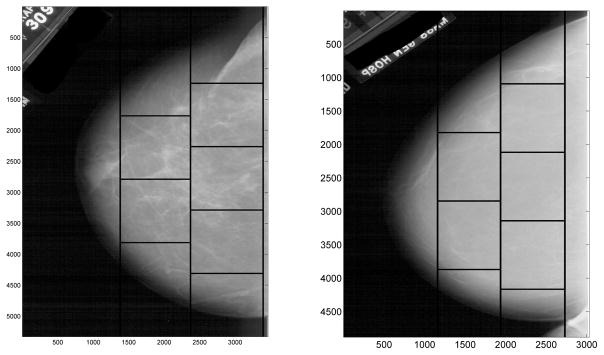
Each image is split into five sub-images, each of size 1024 × 1024 pixels. Dividing the images in this way allows the capturing of only breast tissue, and smaller portions of the image data may be analyzed at a time. Figure 1 shows examples of a mammogram with cancer and one without cancer, split into five sub-images each.

Figure 1.

Mammogram images, with cancer (left) and without cancer (right), split into five sub-images each.

3. Introduction to Wavelets

Wavelets are a mathematical tool for extracting information from different types of data. Often, discussions of wavelets focus on the study of one-dimensional signals, but wavelet techniques may also be applied to the study of multidimensional images; a two-dimensional wavelet transform is presented here. The wavelet transform is similar to the Fourier transform, which represents signals as a summation of sinusoidal building blocks, or basis functions. One key difference, however, is that the wavelet transform is localized in both frequency and time, while the standard Fourier transform is only localized in frequency. In other words, the Fourier transform tells us what frequencies are present in a signal, and the wavelet transform tells us what frequencies are present and when. Wavelets are used for a variety of purposes, including the compression, denoising, and filtering of signals as well as measuring the degree of self-similarity in a signal. An excellent reference is [11]. Statistical aspects of wavelets are discussed in [12] and [13].

Wavelet transforms lead to coefficients (numerical values) representing the nature of a given signal at different locations/resolutions. These coefficients may be used to form the wavelet-based spectra of the signal, showing the relationship between the resolution of the signal and the averaged magnitudes of the coefficients. By assessing the wavelet-based spectra, we may better understand the mathematical characteristics of the overall signal. If the energies (an engineering term for squared coefficients in the wavelet decomposition) decay regularly, this signifies scaling in the data, meaning all resolutions contribute to the overall observed phenomenon. In this case, a measure of regularity can be calculated as the rate of energy decay. More precisely, if the logarithms of average energies in different scales decay linearly with the scale index, then the slope of this decay is describing the regularity of the original signal/object. Thus the spectral slope of the wavelet-based spectra can precisely measure the degree of a signal’s regularity. For details about wavelet-based spectra and their application to assessing regularity of signals/images we direct the reader to [11],[14],[15], and [16].

4. The Scale-Mixing Transform and Spectral Slope

In order to analyze the mammogram images, we apply a 2-D wavelet transform to each of the five non-overlapping 1024 × 1024-pixel regions in both sets of images (cases and controls). For each region, we use the obtained matrix of wavelet coefficients to define the wavelet spectra. There are several ways to define the 2-D wavelet transform. We have selected the scale-mixing wavelet transform (as in [17]), due to its computational and discriminatory properties. For more technical details on the 2-D scale-mixing wavelet transform, see Appendix A. When implementing the transform, the choice of decomposing wavelet is equivalent to the choice of filter. Our experience is that the classification results are generally robust to the choice of wavelet/filter. The Symmlet 8-tap filter is used, as it provides a good compromise between smoothness and locality. These properties of wavelets are both important, but counterpoised.

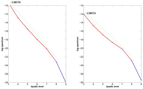
Figure 2 shows the log energy spectra formed for single corresponding regions from the images in Figure 1. As described in the previous section, the decreasing lines are formed by the logarithm of averaged squared wavelet coefficients, or energies, at different scales of the image which are indexed by dyadic level. As the dyadic level increases, the aspects of the image represented are more detailed. The slope measures the change in energy between adjacent dyadic levels of the transformed matrix.

Figure 2.

Log energy spectra for a single region of a case (left) and the log energy spectra for the corresponding region of a control (right)

In this side-by-side analysis, the slope of regressed energies in the diagonal hierarchy across the range of dyadic levels is more negative for the cancerous breast tissue, indicating more regularity. In the one-dimensional case (e.g. time series), high regularity means having long-term positive autocorrelation. In other words, a high value in the series will probably be followed by another high value, and the values a long time into the future will also tend to be high. This concept of regularity may also be translated to the two-dimensional case (e.g. images), as is illustrated in Figure 3.

Figure 3.

Examples of images with low (left), moderate (middle), and high (right) regularity.

In conclusion, the spectral slope of a transformed image represents an informative summary statistic appropriate for classifying images with and without cancer. It is interesting to note that in many biological and medical signals and images, presence of pathology causes signals/images to be more regular, that is, their spectral slopes to be more negative. This is an almost universal phenomenon noted in scaling of EKG, EEG, x-ray radiography, ocular responses, DNA nucleotide signals, etc.

5. Asymmetry Statistics

The scale-mixing transform results in several hierarchies of scales, formed by the matrix of wavelet coefficients. The so-called diagonal hierarchy was used in the previous section to define spectra and assess its informative slope. Adjacent to the diagonal hierarchy on each side there are two hierarchies that measure “fluxes of energies” among coefficients, in which the scale of the x-coordinate differs from the scale of the y-coordinate. By looking at the difference in energies between these two scale-mixing hierarchies we can assess the degree of anisotropy in the image. Specifically, we consider two statistics representative of differences in energies of two diagonally-symmetric mixed detail levels. First, we consider a studentized asymmetry statistic, defined as

$$t_j=\frac{{\overline{e}}_{(j,j+1)}-{\overline{e}}_{(j+1,j)}}{\sqrt{s_{(j,j+1)}^2/n_{(j,j+1)}+s_{(j+1,j)}^2/n_{(j+1,j)}}},$$ (1)

where ē_(j,j+1) and $s_{(j,j+1)}^2$ represent sample mean and variance of squared wavelet coefficients in the tessellation rectangle indexed by scales (j, j + 1). The number of coefficients in this rectangle is n_(j,j+1). For diagonally symmetric rectangle indexed by (j + 1, j), the notation indices j and j + 1 exchange places. Of course, by construction, n_(j,j+1) = n_(j+1,j).

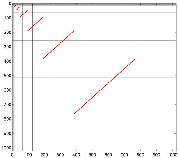
Since wavelets decorrelate, these sets of energies are approximately independent. Since the number of coefficients n_(j,j+1) is typically large, the Central Limit Theorem ensures that the statistic t_j is approximately standard normal under the null hypothesis of isotropy. Figure 4 shows the wavelet coefficients contributing to the statistic in (1), for several values of index j. Note that in regions above the diagonal hierarchy, the level of detail is greater in the horizontal direction than in the vertical direction. In regions below the diagonal hierarchy, the resolution of vertical and horizontal levels is reversed.

Figure 4.

Illustration of wavelet coefficients contributing to the asymmetry statistics. Red lines connect the regions of the wavelet-transformed image used in the calculations, which are above and below the diagonal hierarchy.

In addition to statistic t_j from (1), we consider a fold change asymmetry statistic, defined as

$$f_j=\frac{{\overline{e}}_{(j,j+1)}}{{\overline{e}}_{(j+1,j)}},$$ (2)

where the notation is as in t_j. Use of an asymmetry statistic of this form is motivated by fold change statistics often used in analyzing similarly structured microarray data [18]. When n_(j,j+1) is large, under assumptions of isotropy and independence of wavelet coefficients, the fold statistic in (2) approximately follows a normal distribution with mean 1 and standard deviation $2/\sqrt{n_{(j,j+1)}}$. (To see why this is the case, denote n_(j,j+1) = n_(j+1,j) simply as n. Under the assumption of isotropy, nē_(j,j+1) and nē_(j+1,j) are approximately independent ${\chi }_n^2$, as sums of squares of zero-centered wavelet coefficients. Under the fractional Brownian motion (fBm) model, the Gaussianity and approximate independence of wavelet coefficients follows from [19]. Thus, the ratio f_j is approximately F-distributed, f_j ~ F_n,n, with mean $\frac{n}{n-2}$ and variance $\frac{2n^2(2n-2)}{n{(n-2)}^2(n-4)}$ . For n large, the mean approaches 1 and variance behaves as $\frac{4}{n}$. Also, for n large, F_n,n can be approximated by a normal distribution, due to Central Limit Theorem for exchangeable random variables.)

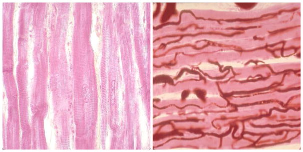
In order to demonstrate how directional (in this case vertical and horizontal) features in an image may be captured through an asymmetry statistic, we compute the asymmetry statistics for two highly anisotropic 256 × 256 pixel images of cardiac tissue [20]. The two images, one of central nuclei and striations having strong vertical features and one of skeletal muscle vasculature having strong horizontal features, are shown in Figure 5. The asymmetry statistics at various dyadic level pairings for these two images are displayed in Table 1. The lower dyadic level pairings represent more coarse features of each image, while the higher dyadic level pairings represent more fine features of each image. The systematic differences in asymmetry statistics may be seen for the coarser level pairings (j = 2, 3, and 4). The finer level pairings (j = 5, 6) are not capable of “seeing” the images’ directional differences.

Figure 5.

Images with strong directional features: vertical (left) and horizontal (right).

Table 1.

Comparison of the asymmetry statistics for images with strong vertical and horizontal features by (j, j + 1)−(j + 1, j) pairing. The systematic differences in asymmetry statistics may be seen for the coarser level pairings (j = 2, 3, and 4). Some finer level pairings (j = 5, 6) may not be capable of “seeing” the images’ directional differences, e.g. t₅ for horizontal, and t₆ for vertical.

	j = 2	j = 3	j = 4	j = 5	j = 6
Studentized Asymmetry Statistic tj
Figure 5 (left): Vertical	2.5219	2.6747	4.3881	4.4380	0.5748
Figure 5 (right): Horizontal	−1.9690	−4.1924	−3.9102	1.0322	4.7830
Fold Change Asymmetry Statistic fj
Figure 5 (left): Vertical	2.9400	2.0928	1.9648	1.3481	1.0251
Figure 5 (right): Horizontal	0.3920	0.3025	0.3284	1.0980	1.1780

Referring back to Figure 4, the studentized asymmetry statistics for the image with prominent vertical features are positive and the fold change asymmetry statistics are greater than 1, meaning there is more energy in regions above the diagonal hierarchy. In contrast, the studentized asymmetry statistics for the image with prominent horizontal features are negative and the fold change asymmetry statistics are less than 1, meaning there is more energy in regions below the diagonal hierarchy.

As we pointed out, distributions of the asymmetry statistics are well approximated by normal distribution when n_(j,j+1) is large, which is the case for j = 5, 6. When level j is coarse, the distributions of asymmetry statistics are impacted by dependence, skewness, and choice of wavelet. In order to calibrate the asymmetry statistics in such cases, we may find the degree of deviation from isotropy (uniformity in all orientations) via parametric bootstrap: We simulate a large number (say 1,000) of fractional Brownian fields (fBfs) with the same spectral slope as the image to be analyzed. Fractional Brownian fields are theoretical spatial processes that can mimic the diagonal spectral slope, but possess isotropy, and theoretically the asymmetry statistics should not be significant. Next, we find the empirical bootstrap distributions of each asymmetry statistic from simulated fields. Finally, we evaluate where in these bootstrap distributions the actual image’s asymmetry statistics fall by computing associated achieved significance levels (ASLs). The ASLs are analogous to p-values, with values close to zero indicating significant deviation from isotropy.

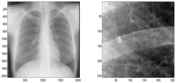
For example, consider the 256 × 256 portion of the chest radiograph shown in Figure 6 [21]. First, we find the spectral slope (−2.8529) and generate 1,000 fBfs with the same slope. We then compute asymmetry statistics corresponding to each fBf and generate the empirical bootstrap distributions of the asymmetry statistics at the three coarsest scale levels. Figures 7 and 8 show these bootstrap distributions (histograms) and where the actual image’s asymmetry statistics fall in the distributions (red vertical lines). This chest radiograph has asymmetry statistics falling in the left tails of the distributions, indicating high horizontal directionality (t statistic ASLs (coarse to fine): 0.061, 0.001, 0; f statistic ASLs (coarse to fine): 0.051, 0, 0). Therefore, the asymmetry statistics pick up the coarse horizontal directionality of the rib contour in the image.

Figure 6.

Chest radiograph (left) and the portion analyzed for deviation from isotropy (right)

Figure 7.

Empirical bootstrap distributions (histograms) for the t statistic at the three coarsest levels and where the chest radiograph subimage’s asymmetry statistics fall in the distributions (red vertical lines). This image has asymmetry statistics falling in the left tails of the distributions, indicating high horizontal directionality (t statistic ASLs (coarse to fine): 0.061, 0.001, 0).

Figure 8.

Empirical bootstrap distributions (histograms) for the f statistic at the three coarsest levels and where the chest radiograph subimage’s asymmetry statistics fall in the distributions (red vertical lines). This image has asymmetry statistics falling in the left tails of the distributions, indicating high horizontal directionality (f statistic ASLs (coarse to fine): 0.051, 0, 0).

6. Comparing Descriptors for Cases and Controls

As mentioned in section 4, the spectral slope is typically more negative for the mammograms with cancer than for the mammograms without cancer. However, from each mammogram 5 subimages are taken, thus increasing the sample size, but inducing dependence. In order to quantify the influence of any descriptor distilled from mammograms on the disease status, we perform a two-way nested ANOVA, under the model

$$y_{\mathit{ijk}}=\mu +{\alpha }_i+{\beta }_{j(i)}+{\epsilon }_{\mathit{ijk}},{\epsilon }_{\mathit{ijk}}=N(0,{\sigma }^2),$$ (3)

with standard identifiability constraints Σ_i α_i = 0, Σ_j β_j(i) = 0, i = 1, 2.

In (3), y_ijk represents the spectral slope for each possible region of each mammogram, α_i, i = 1, 2 represents the effect of case/control on the slope, and β_j(1), j = 1, …, 79 and β_j(2), j = 1, …, 45 represent effects of subjects on the slope for the cases and controls, respectively. This analysis separately models the effects of the subject and whether the mammogram belongs to the cancerous group. We assume that scaling is independent across subregions, accounting for the status (α_i) and the subject nested in the status (β_j(i)). Table 2 contains the two-way nested ANOVA results, showing that cases and controls produce significantly different spectral slopes (effects α̂₁ = −0.0462 for the cases, and α̂₂ = 0.0462 for the controls). This model accounted for significant differences in spectral slopes among subjects not relevant to the disease status. For our classification procedure, we use slopes y_ijk − ε̂_ijk to represent each image.

Table 2.

Two-way nested ANOVA on spectral slopes

Source	SS	df	MS	F	Prob>F
Case/Control	1.2251	1	1.22511	8.39	0.0045
Subject(Case/Control)	17.821	122	0.14607	6.53	0
Error	11.0909	496	0.02236
Total	30.137	619

We fit analogous two-way nested ANOVA models for values of both the studentized asymmetry statistic and the fold change asymmetry statistic at each detail level. For both asymmetry statistics, cases and controls produce significantly different values at all but the coarsest levels of detail. Both t and f statistics tend to be higher for cases compared to controls. The subject effect is significant for each asymmetry statistic at every detail level. Tables 3 and 4 contain the two-way nested ANOVA results for values of the t and f statistics, respectively, at dyadic level pairing 5 and 6 (as an example). For this level pairing, the fitted t statistic coefficients are ${\widehat{\alpha }}_1^{\ast }=0.4660$ for cases and ${\widehat{\alpha }}_2^{\ast }=-0.4660$ for controls. The fitted f statistic coefficients are ${\widehat{\alpha }}_1^{\ast \ast }=0.0219$ for cases and ${\widehat{\alpha }}_2^{\ast \ast }=-0.0219$ for controls. As with slopes, we use asymmetry statistic values with subtracted fitted residuals to represent each image.

Table 3.

Two-way nested ANOVA on t statistics

Source	SS	df	MS	F	Prob>F
Case/Control	124.52	1	124.52	5.4	0.0218
Subject(Case/Control)	2814.36	122	23.069	3.1	0
Error	3696.7	496	7.453
Total	6635.58	619

Table 4.

Two-way nested ANOVA on f statistics

Source	SS	df	MS	F	Prob>F
Case/Control	0.2739	1	0.2739	7.24	0.0081
Subject(Case/Control)	4.6145	122	0.03782	3.05	0
Error	6.1441	496	0.01239
Total	11.0325	619

7. Classification Results

To classify subjects on the basis of derived features from their mammograms, we employed Support Vector Machines (SVM) [22]. An SVM is a discriminative classifier formally defined by a separating hyperplane. Given labeled training data (supervised learning), the SVM algorithm outputs an optimal hyperplane which categorizes new subjects; an excellent reference is [23]. Table 5 displays the SVM classification results by choice of kernel (linear, quadratic, or radial basis) with and without asymmetry statistics for 1,000 iterations. For each iteration, the data set is split into a 70% training set (87 images) and a 30% testing set (37 images). For each procedure, the spectral slopes are used as features to train the model. The addition of asymmetry statistics of either form as features in the classification significantly raises the specificity and overall accuracy. The best results using only spectral slopes in the classification are obtained using the linear kernel (accuracy = 62.68%). The best overall results are achieved using the linear kernel and including both spectral slopes and fold change asymmetry statistics in the classification (accuracy = 76.59%).

Table 5.

SVM classification results. The best results are achieved using the linear kernel and including both spectral slopes and fold change asymmetry statistics in the classification.

	Mean Accuracy Rate	Mean Sensitivity	Mean Specificity
Slopes Only
Linear	0.6268	0.7039	0.4952
Quadratic	0.6027	0.6855	0.4607
Radial Basis	0.6017	0.5978	0.6099
Slopes + Asymmetry t
Linear	0.6731	0.6685	0.6819
Quadratic	0.6684	0.6930	0.6314
Radial Basis	0.6332	0.6901	0.5474
Slopes + Asymmetry f
Linear	0.7659	0.7250	0.8379
Quadratic	0.7195	0.7414	0.6856
Radial Basis	0.7296	0.7800	0.6513

The performance of logistic regression as a classification tool was also assessed, but this classifier consistently performed worse than the SVM classifier with linear kernel by around three percentage points in accuracy. For example, the logistic regression model with spectral slopes and fold change asymmetry statistics as inputs resulted in a classification procedure with 73.68% accuracy (sensitivity = 71.85%, specificity = 77.96%). Typically, in our experience, logistic regression and SVM with linear kernel perform comparably. However, when features are correlated, SVMs can be superior [24]. The correlation among fold change values for a single image could explain the slight difference in the performance of the two classifiers in this case.

8. Conclusion

Mammography is routinely used to screen for breast cancer. However, the interpretation of mammograms by radiologists is made difficult by the heterogeneous nature of normal breast tissue and the fact that cancers are often of the same radiographic density as normal tissue. CAD algorithms have been developed to assist in the identification of suspicious regions. However, most CAD algorithms rely on pattern recognition and attempt to identify predefined physical characteristics of calcification, masses, and important asymmetries. Wavelet based scaling makes no a priori assumptions about the morphology of a cancer, but rather detects it by departure from normal background. By using scaling properties of mammogram images, we have captured information contained in the background tissue of images which is not utilized when only considering lesion morphology. Using features based on spectral slopes and our defined asymmetry statistics, we have achieved an SVM classification procedure with 76.59% accuracy on the testing sample. Importantly, the mammograms of both the cases and controls were performed on the same mammography unit, so this level of separation is not due to any image acquisition effect. We suggest that this classifier may be used in conjunction with other methodologies in order to improve the detection of breast cancer through mammography. If the tool proves robust on further investigation, it may be useful in outlining cases that require heightened scrutiny or even addition of supplemental screening modalities, especially in cases where the patient has dense background parenchymal tissue, a factor known to decrease mammographic sensitivity.

9. Appendix A: The 2-D Scale-Mixing Wavelet Transform

The 2-D wavelet basis functions for the 2-D wavelet transform are constructed via translations and dilations in a product of univariate wavelet and scaling functions

$$\begin{array}{lll}\hfill \varphi (t_1,t_2)& =\hfill & \varphi (t_1)\varphi (t_2)\hfill \\ \hfill {\psi }^h(t_1,t_2)& =\hfill & \varphi (t_1)\psi (t_2)\hfill \\ \hfill {\psi }^v(t_1,t_2)& =\hfill & \psi (t_1)\varphi (t_2)\hfill \\ \hfill {\psi }^d(t_1,t_2)& =\hfill & \psi (t_1)\psi (t_2),\hfill \end{array}$$ (4)

where the symbols h, v, d stand for horizontal, vertical and diagonal directions, respectively, since the atoms capture image features in the corresponding directions.

Consider the wavelet atoms

$$\begin{array}{lll}{\varphi }_{(j_1,j_2),\mathbf{k}}(\mathbf{t})\hfill & =\hfill & 2^{(j_1+j_2)/2}\varphi (2^{j_1}{t}_1-k_1,2^{j_2}{t}_2-k_2)\hfill \end{array}$$ (5)

$$\begin{array}{lll}{\psi }_{(j_1,j_2),\mathbf{k}}^i(\mathbf{t})\hfill & =\hfill & 2^{(j_1+j_2)/2}{\psi }^i(2^{j_1}{t}_1-k_1,2^{j_2}{t}_2-k_2),\hfill \end{array}$$ (6)

where i is one of h, v, or d, as in (4) and (j₁, j₂) ∈ ℤ², then any function X ∈ ℒ₂(ℝ²) can be represented as

$$\begin{array}{lll}X(\mathbf{t})\hfill & =\hfill & \sum _{\mathbf{k}}{c}_{(J_0,J_0),\mathbf{k}}{\varphi }_{(J_0,J_0),\mathbf{k}}(\mathbf{t})\hfill \\ \hfill & +\hfill & \sum _{j>J_0}\sum _{\mathbf{k}}{d}_{(J_0,j),\mathbf{k}}{\psi }_{(J_0,j),\mathbf{k}}^h(\mathbf{t})\hfill \\ \hfill & +\hfill & \sum _{j>J_0}\sum _{\mathbf{k}}{d}_{(j,J_0),\mathbf{k}}{\psi }_{(j,J_0),\mathbf{k}}^v(\mathbf{t})\hfill \\ \hfill & +\hfill & \sum _{j_1,j_2>J_0}\sum _{\mathbf{k}}{d}_{(j_1,j_2),\mathbf{k}}{\psi }_{(j_1,j_2),\mathbf{k}}^d(\mathbf{t}),\hfill \end{array}$$

and the 2-D scale-mixing wavelet transform is obtained. Notice that (j₁, j₂) in (5) and (6) can be indexed as well as (j₁, j₁ + s), where s ∈ ℤ. The scale-mixing detail coefficients are defined as

$$\begin{array}{lll}{d}_{(J_0,j),\mathbf{k}}\hfill & =\hfill & 2^{(J_0+j)/2}\int X(\mathbf{t}){\psi }^h(2^{J_0}{t}_1-k_1,2^j{t}_2-k_2)d{t}_{1}d{t}_2,\hfill \\ d_{(j,J_0),\mathbf{k}}\hfill & =\hfill & 2^{(j+J_0)/2}\int X(\mathbf{t}){\psi }^v(2^j{t}_1-k_1,2^{J_0}{t}_2-k_2)d{t}_{1}d{t}_2,\hfill \\ d_{(j_1,j_2),\mathbf{k}}\hfill & =\hfill & 2^{(j_1+j_2)/2}\int X(\mathbf{t}){\psi }^d(2^{j_1}{t}_1-k_1,2^{j_2}{t}_2-k_2)d{t}_{1}d{t}_2.\hfill \end{array}$$ (7)

The scale-mixing detail coefficients are linked to the original image (2-D time series) through a matrix equation. Suppose that a 2ⁿ × 2ⁿ image (matrix) A is to be transformed into the wavelet domain. If the rows of A are transformed by a one-dimensional transform given by the 2ⁿ × 2ⁿ wavelet matrix W, then the object WA′ represents a matrix in which the columns are transformed rows of A. If the same is repeated on the rows of WA′ the result is

$$B=W{(W{A}^{\prime })}^{\prime }=WA{W}^{\prime }.$$ (8)

Matrix B will be called the scale-mixing transform of matrix A, and will be the basis for defining the scale-mixing spectra. The scale-mixing wavelet transform was previously used in the literature, but not as extensively as the traditional 2-D transform. Some references are [25, 26, 17, 27]. It is also known as “hyperbolic” [27] and “rectangular” [26]. In its complex version this transform was utilized in [28].

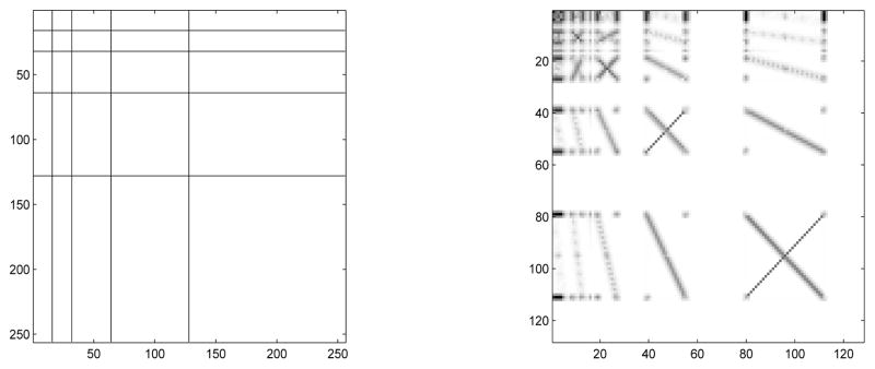
Figure 9 illustrates the 2-D scale-mixing wavelet transform, using the box with cross image. The scale-mixing 2-D transform is operationally appealing. The images are usually of moderate size and constructing appropriate W is computationally fast. Since W is orthogonal, the inverse transform is straightforward,

Figure 9.

Tessellations for some 2-D scale-mixing wavelet transform of depth 4 (left), and 2-D scale-mixing wavelet transform of the box with cross image (right).

$$A=W^{\prime }BW.$$

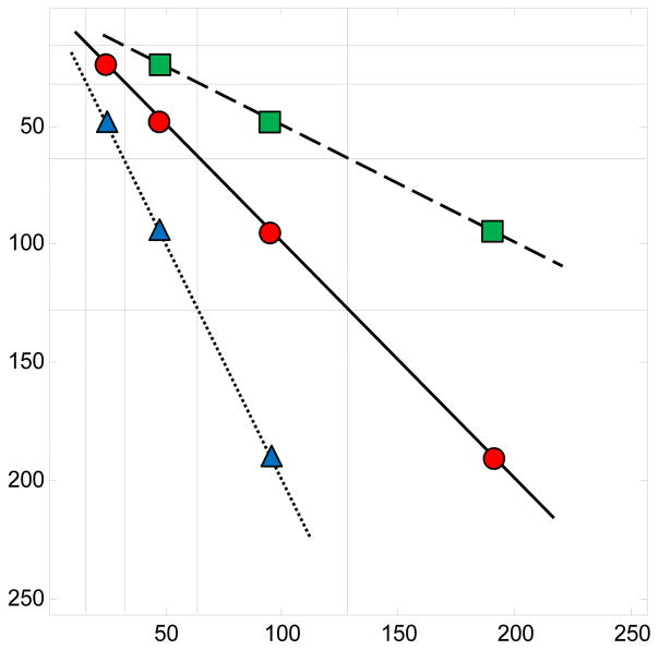
By inspecting the tessellation in Figure 9 (left), several hierarchies of detail spaces can be identified. The diagonal hierarchy interfaces coefficients with the same component scales and coincides with the diagonal hierarchy in the traditional 2-D spectrum. Just above and below the diagonal hierarchy are hierarchies of detail spaces that interface the scales that differ by 1. For example, for the hierarchy above the diagonal, the scales along x-direction are interfaced by the next coarser scale along y-direction. For the hierarchy below the diagonal, the roles of x and y are interchanged. Figure 10 (a) shows three hierarchies of detail coefficients: the diagonal hierarchy (circles) and the hierarchies in which dyadic scales differ by 1 (triangles and squares).

Figure 10.

Three detail-space hierarchies generating the scale-mixing 2-D transform, where (j₁, j₂) is indexed as (j, j + s), s ∈ ℤ. Circles correspond to s = 0, triangles to s = 1, and squares to s = −1;

9.1. Definition of Scale-Mixing Wavelet Spectra

The scale-mixing spectrum is defined in terms of the scale-mixing coefficients (7) as

$$S(j,s)={log}_2\mathbb{E}\left(d_{(j,j+s),\mathbf{k}}^2\right),$$ (9)

where s ∈ ℤ is fixed. The empirical counterpart of (9) is

$$\widehat{S}(j,s)={log}_2\left(\overline{d_{(j,j+s),\mathbf{k}}^2}\right).$$ (10)

In (10), $\overline{d_{(j,j+s),\mathbf{k}}^2}$ denotes the average of squared detail coefficients (7) at level (j, j + s). Notice that the case s = 0 in (10) corresponds to the traditional diagonal 2-D spectrum, see Figure 10.

References

- 1.Siegel R, Naishadham D, Jemal A. Cancer statistics. CA Cancer J Clin. 2013;63(1):11–30. doi: 10.3322/caac.21166. [DOI] [PubMed] [Google Scholar]
- 2.National Cancer Institute. Mammograms fact sheet. 2014 http://www.cancer.gov/cancertopics/types/breast/mammograms-fact-sheet.
- 3.Carney P, Miglioretti D, Yankaskas B, Kerlikowske K, Rosenberg R, Rutter C, Geller B, Abraham L, Taplin S, Dignan M, et al. Individual and combined effects of age, breast density, and hormone replacement therapy use on the accuracy of screening mammography. Ann Intern Med. 2003;138(3):168–175. doi: 10.7326/0003-4819-138-3-200302040-00008. [DOI] [PubMed] [Google Scholar]
- 4.Houssami N, Irwig L, Ciatto S. Radiological surveillance of interval breast cancers in screening programmes. The Lancet Oncology. 2006;7(3):259–265. doi: 10.1016/S1470-2045(06)70617-9. [DOI] [PubMed] [Google Scholar]
- 5.Freer TW, Ulissey MJ. Screening mammography with computer-aided detection: Prospective study of 12,860 patients in a community breast center. Radiology. 2001;220(3):781–786. doi: 10.1148/radiol.2203001282. [DOI] [PubMed] [Google Scholar]
- 6.Chan HP, Goi K, Galhotra S, Vyborny CJ, MacMahon H, Jokich PM. Image feature analysis and computer-aided diagnosis in digital radiography. I. Automated detection of microcalcifications in mammography. Medical Physics. 1987;14(4):538–548. doi: 10.1118/1.596065. [DOI] [PubMed] [Google Scholar]
- 7.Cheng HD, Cai X, Chen X, Hu L, Lou X. Computer-aided detection and classification of microcalcifications in mammograms: A survey. Pattern Recognition. 2003;36(12):2967–2991. [Google Scholar]
- 8.Jeon S, Nicolis O, Vidakovic B. Mammogram diagnostics via 2-D complex wavelet-based self-similarity measures. SP Journal of Mathematical Sciences. 2014;8(2):265–284. [Google Scholar]
- 9.Heath M, Bowyer K, Kopans D, Moore R, Kegelmeyer WP. The digital database for screening mammography. Proceedings of the Fifth International Workshop on Digital Mammography. 2001:212–218. [Google Scholar]
- 10.Heath M, Bowyer K, Kopans D, Kegelmeyer WP, Moore R, Chang K, Kumaran SM. Current status of the digital database for screening mammography. Proceedings of the Fourth International Workshop on Digital Mammography. 1998:457–460. [Google Scholar]
- 11.Mallat S. A Wavelet Tour of Signal Processing: The Sparse Way. Academic Press; Waltham, MA: 2009. [Google Scholar]
- 12.Vidakovic B. Statistical Modeling by Wavelets. John Wiley & Sons; 1999. [Google Scholar]
- 13.Nason GP. Wavelet Methods in Statistics with R. Springer; New York: 2008. [Google Scholar]
- 14.Doukhan P, Oppenheim G, Taqqu MS, editors. Theory and Applications of Long-Range Dependence. Birkhäuser; 2003. [Google Scholar]
- 15.Ramírez P, Vidakovic B. A 2-D wavelet-based multiscale approach with applications to the analysis of digital mammograms. Computational Statistics and Data Analysis. 2013;58:71–81. http://dx.doi.org/10.1016/j.csda.2011.09.009. [Google Scholar]
- 16.Nicolis O, Ramírez P, Vidakovic B. 2-D wavelet-based spectra with applications. Computational Statistics & Data Analysis. 2011;55(1):738–751. [Google Scholar]
- 17.Ramírez-Cobo P, Lee KS, Molini A, Porporato A, Katul G, Vidakovic B. A wavelet-based spectral method for extracting self-similarity measures in time-varying two-dimensional rainfall maps. Journal of Time Series Analysis. 2011;32(4):351–363. [Google Scholar]
- 18.Tibshirani R. A comparison of fold-change and the t-statistic for microarray data analysis. Analysis. 2007:1–17. [Google Scholar]
- 19.Flandrin P. Wavelet analysis and synthesis of fractional Brownian motion. IEEE Trans Information Theory. 1992;38(2):910–917. [Google Scholar]
- 20.University of Delaware Department of Biological Sciences. Images of cardiac tissue. 2015 http://www.udel.edu/biology/Wage/histopage/colorpage/cmu/cmu.htm.
- 21.Emory University School of Medicine PACS. Chest radiographs. [Google Scholar]
- 22.Vapnik VN. Statistical Learning Theory. John Wiley & Sons; 1998. [Google Scholar]
- 23.Hastie T, Tibshirani R, Friedman J. The Elements of Statistical Learning: Data Mining, Inference, and Prediction. 2. Springer; 2009. [Google Scholar]
- 24.Toloşi L, Lengauer T. Classification with correlated features: Unreliability of feature ranking and solutions. Bioinformatics. 2014;27(14):1986–1994. doi: 10.1093/bioinformatics/btr300. [DOI] [PubMed] [Google Scholar]
- 25.Neumann MH, von Sachs R. Wavelet thresholding in anisotropic function classes and application to adaptive estimation. Annals of Statistics. 1997;25(1):38–76. [Google Scholar]
- 26.Zavadsky V. Image approximation by rectangular wavelet transform. Journal of Mathematical Imaging and Vision. 2007;27(2):129–138. [Google Scholar]
- 27.Roux SG, Clausel M, Vedel B, Jaffard S, Abry P. Self-similar anisotropic texture analysis: The hyperbolic wavelet transform contribution. IEEE Transactions on Image Processing. 2013;22(11):43534363. doi: 10.1109/TIP.2013.2272515. [DOI] [PubMed] [Google Scholar]
- 28.Reményi N, Nicolis O, Nason G, Vidakovic B. Image denoising with 2-D scale-mixing complex wavelet transforms. IEEE Transactions on Image Processing. 2014;23(12):5165–5174. doi: 10.1109/TIP.2014.2362058. [DOI] [PubMed] [Google Scholar]