Detecting Cardiovascular Disease from Mammograms with Deep Learning

Abstract

Coronary artery disease is a major cause of death in women. Breast arterial calcifications (BACs), detected in mam-mograms, can be useful risk markers associated with the disease. We investigate the feasibility of automated and accurate detection of BACs in mammograms for risk assessment of coronary artery disease. We develop a twelve-layer convolutional neural network to discriminate BAC from non-BAC and apply a pixel-wise, patch-based procedure for BAC detection. To assess the performance of the system, we conduct a reader study to provide ground-truth information using the consensus of human expert radiologists. We evaluate the performance using a set of 840 full-field digital mammograms from 210 cases, using both free-response receiver operating characteristic (FROC) analysis and calcium mass quantification analysis. The FROC analysis shows that the deep learning approach achieves a level of detection similar to the human experts. The calcium mass quantification analysis shows that the inferred calcium mass is close to the ground truth, with a linear regression between them yielding a coefficient of determination of 96.24%. Taken together, these results suggest that deep learning can be used effectively to develop an automated system for BAC detection in mammograms to help identify and assess patients with cardiovascular risks.

I. Introduction

Cardiovascular disease is the first cause of mortality in women in the world [1]. Coronary artery disease is one of the most common types of cardiovascular disease, leading to 1 out of 7 deaths in the United States [2]. Various studies have demonstrated that breast arterial calcifications (BACs), detected on mammogram images, can be a useful risk marker for coronary artery disease [3, 4]. For example, Pecchi et al. [5] and Matsumura et al. [6] independently studied the association between BACs in mammograms and coronary artery calcifications (CACs) quantified by multislice CT and found a strong correlation between them. Maas et al. [7] investigated whether BACs on mammograms can predict future development of CACs and showed that BACs are predictive of subsequent development of CACs. Thus automated identification of BACs in mammograms could provide a cost-and labor- effective strategy for the risk assessment of coronary artery disease and subsequent triage in women.

BACs are calcium deposits which line up the walls of the arteries in the breast. As shown in Figure 1, they appear as parallel or tubular tracks on mammograms [8], which are taken very frequently. Indeed, mammography is a routine screening tool for detection and diagnosis of breast cancer in women. The American Cancer Society recommends that women 40 years and older undergo annual mammography screening [9]. It is estimated that nearly 40 million mammography exams are performed annually in the United States alone [10]. However, BACs detected in mammograms are considered to be irrelevant for the diagnosis of breast cancer [11], and thus are treated as false positives (FPs) and are not reported in current mam-mography screenings. Rather than discarding this information, the automated detection of BACs in mammograms could take advantage of routine mammography screening.

Fig. 1.

(a) Examples of regions of interest (ROIs) cropped from mammograms containing BACs; (b) the corresponding BACs associated with the ROIs, with BAC boundaries marked by red contours. For better visualization, a background removal process is applied to each ROI; the background of a pixel is estimated as the average intensity of its circular neighborhood with a radius of 50 pixels.

In spite of the advantages mentioned above, in most (if not all) clinical studies to date [4, 12, 11], BACs in mammograms were manually detected by radiologists. Such manual process is necessary in the early stages of technology development, but it is time-consuming, subjective, and tedious, thus hampering large-scale clinical testing and deployment of this new screening approach. Therefore, it is now becoming essential to develop computerized algorithms for the automated detection of BACs in mammograms. Moreover, besides cardiovascular disease [13, 14], BACs are also useful biomarkers associated with chronic kidney disease [15], bone mineral density reduction [16], diabetes [17], hypertension [18], and stroke and heart failure [3]. Therefore, automated detection of BACs can be helpful in diagnosis of multiple diseases. In addition to the application to these non-cancer diseases [19, 20, 21], the automated detection of BACs in mammograms could also be used to improve microcalcification (MC) detection for breast cancer itself, essentially by subtracting BACs from the images [8, 22].

Given the growing interest, several algorithms have been proposed for BAC detection in the literature. For example, Cheng et al. [19, 20, 21] developed a two-step procedure by considering both the calcification and vesselness cues, using first a tracking method with uncertainty scheme to generate multiple sampling paths, and then applying a compiling and linking algorithm to group the resulting BAC paths into BACs. Ge et al. [8] adopted a k-segments clustering algorithm to model BACs in the vessel walls as line segments during BAC detection, and then subtracted these BACs during MC detection for breast cancer screening. Finally, Mordang et al. [22] applied a GentleBoost classifier to remove BACs as FPs in MC detection by a set of manually designed features, including shape, topology and texture.

Despite these efforts, the accurate and automated detection of BACs in mammograms remains an unsolved task and the technology is far from clinical deployment. This is primarily because BACs in mammograms vary in size, shape, and contrast. For example, in Figure 1(a) we show three regions of interest (ROIs) cropped from mammograms, all containing BACs; and in Figure 1(b) we show the corresponding BACs with contour boundaries marked by radiologists. In these figures, BACs appear as bright spots forming elongated patterns along the walls of the arteries in the breast; however, these patterns vary considerably and can be long and strong (left), intersected with each other (left), short and weak (middle), or disconnected along an artery (right).

In recent years [23], neural networks and deep learning have been used to successfully tackle a variety of problems in engineering, ranging from computer vision [24, 25, 26, 27] to speech recognition [28], as well as in the natural sciences, in areas ranging from high energy physics [29, 30], to chemistry [31, 32, 33], and to biology [34, 35, 36]. Convolutional neural network architectures [37, 38] in particular have led to several successful pattern classification and detection in natural images [24, 25, 27]. Thus it is natural to consider applying deep learning methods also to biomedical images. For example, in [39] a deep learning architecture was applied to each pixel to address problems of membrane segmentation in electron microscopy images; in [40] a deep convolutional neural network (CNN) was used as the 2nd tier in a two-tiered, coarse-to-fine cascade framework, to refine the candidate lesions from the first tier for sclerotic spine metastases detection in CT images; in [41] a multi-scale CNN was developed for lung nodule detection in CT images; and in [42] a GoogLeNet-based method was adopted for automated detection and diagnosis of metastatic breast cancer in whole slide images of sentinel lymph node biopsies.

In this study, we investigate the feasibility of automated and accurate BAC detection on mammograms by deep learning methods in support of the long-term goal of developing an automated BAC detector which can be used to provide risk markers for coronary artery disease [3, 4, 12]. We formulate the problem as a pixel-wise, patch-based two-class classification problem. That is, for any pixel under consideration, we utilize an image patch around it. The image patches are fed to a deep CNN which is trained to classify whether the central pixel belongs to the BAC class or not. Compared to other machine learning and other algorithms, the deep CNN can extract features automatically while achieving good classification performance. It has been demonstrated that features automatically learnt by deep CNNs tend to outperform features that are handcrafted by human experts [43, 44].

II. Methods

A. Deep convolutional neural network architecture

The deep CNN architecture considered in this study consists of a cascade of several convolutional (Conv), batch normalization, nonlinearity, max-pooling (Pooling), and fully connected (FC) layers. Each convolutional layer is followed by a batch normalization layer and a nonlinearity layer. In Table I, we illustrate the architecture used, in which the batch normalization layer and nonlinearity layer following each convolutional layer are omitted to save space. This leads to a 12-layers neural network, consisting of 10 convolutional layers and two fully connected layers. The convolutional layers can be viewed as feature extractors, while the fully connected layers are used for the final classification.

Table I.

Architecture of the deep CNN used in this study. Each convolutional layer is followed by a batch normalization layer and a nonlinearity layer, omitted here to save space. In total, there are 10 convolutional layers and two fully connected layers.

Layer	# filters	Size	Output size
input	-	-	95 × 95
Conv	32	3×3	95 × 95
Conv	16	3×3	95 × 95
Pooling	-	3×3s2	47 × 47
Conv	64	3×3	47 × 47
Conv	32	3×3	47 × 47
Pooling	-	3×3s2	23 × 23
Conv	128	3×3	23 × 23
Conv	128	3×3	23 × 23
Conv	128	3×3	23 × 23
Pooling	-	3×3s2	11 × 11
Conv	256	3×3	11 × 11
Conv	128	3×3	11 × 11
Conv	128	3×3	11 × 11
Pooling	-	3×3s2	5×5
FC	128	-	128
FC	2	-	2

In the development phase, we experimented with many other architectures and in Table I we report only the one with lowest classification error for the samples in the validation set (see Section III-C). The architecture has a sequence of 2, 2, 3, and 3 convolutional layers before the four max-pooling layers, respectively. In one experiment, for instance, we started from an architecture with seven layers, which includes a sequence of 1, 1, 1, and 2 convolutional layers before the four max-pooling layers. We then gradually increased the number of convolutional layers and stopped when no further improvement was observed.

Convolutional layers generate an output feature map by convolving the input feature map with a set of convolution filters implemented by weight sharing. Typically, in deep CNNs, the majority of the trainable parameters are associated with convolutional layers. In this study, the size of 3 × 3 is used for all of the convolutional filters as illustrated in Table I.

Batch normalization layers are introduced to deal with the internal covariate shift, which refers to the phenomenon that the distribution of each layer's inputs changes during training when the parameters of the previous layers change [45]. It independently achieves z-score normalization on each feature in the feature maps, so that each resulting feature has zero mean and unit standard deviation. The mean and standard deviation for the z-score normalization are estimated from all the samples in each training batch. This batch normalization has been shown to speed up learning and improve classification performance [45].

Nonlinearity layers are implemented by associating a nonlinear activation function with the corresponding neurons. Unlike the convolutional and batch normalization layers which produce linear transformations, these layers produce a nonlinear transformation, ultimately yielding a highly non-linear classifier. In this study, we use leaky rectified linear units (ReLU) [46] with leakiness of 0.5.

Max-pooling layers summarize the outputs of neighboring regions in the same feature map. The output of a max-pooling unit corresponds to the maximum of its input features, taken over a certain region. In this study, the output is generated for every other location (i.e. with stride 2) by considering the 3 × 3 neighborhood region of the location, denoted as 3×3s2 in Table I.

Fully connected layers correspond to pairs of consecutive layers with full connectivity between all the corresponding units. All the connection weights are trainable.

After the last fully connected layer, a softmax activation function [25] is employed, the output of which can be interpreted as the probability that the pixel at the center of the initial input belongs to a BAC.

In total, the architecture has around 1.51 million parameters to be trained. These are trained by stochastic gradient descent to minimize the cross entropy between true class labels and predicted class labels, together with standard L2 regularization.

To further avoid potential overfitting problems, dropout [47, 48] is applied to the input of the first fully-connected layer. Dropout can be viewed as a regularization technique, which randomly drops neural units from the neural network with a certain probability during training. In this study, dropout with probability 0.5 is used.

B. Testing

During testing, for each mammogram image in the test set, the optimal CNN model is applied to each pixel in the tissue region of the image (value 0 is assigned to the pixels out of the tissue region, since they cannot belong to BAC regions), yielding a probability map with the same size as the image under consideration. The value of each pixel in the probability map indicates the probability of that pixel being in the BAC class.

When a pixel is close to the image border, its corresponding feature input (i.e. the image patch centered around it) includes pixels outside the image, thus image padding is required. In this study, we use a symmetric image padding scheme.

The tissue region of an image is obtained as the largest connected region with intensity value larger than the mean intensity of the whole image. A morphology open operator with circular structuring element of diameter 21 pixels is used to smooth the boundary of the tissue region.

C. Postprocessing

BACs can be detected by a thresholding method, that is, by applying a threshold to the probability map obtained in Section II-B. However, the BACs obtained with such method tend to be too wide, especially when the threshold is low. To mitigate this effect and obtain accurate BAC detections, we consider a post-processing procedure as follows. For a candidate BAC obtained from the thresholding method, we first extract its skeleton, and then apply a morphology dilation operator to the skeleton, such that the dilated region has a width of 2.1 mm, the typical width of a breast artery. Finally, the BAC is detected as the overlapping region between the candidate BAC produced by the thresholding methods, and its dilated skeleton region. In the experiments, the skeleton of a region is mainly obtained by the pattern thinning algorithm in [49]; to refine the thinned pattern for BACs, we further remove its small branches and extend its two endpoints.

III. Experiments

A. Dataset

In this study, we make use of a set of 840 standard screening full-field digital mammograms (FFDMs) from 210 cases. Each case includes mammography images from four standard views: a cranial-caudal (CC) view and a mediolateral-oblique (MLO) view, from both the left and right breasts. All the mammogram images were collected at 9 Kaiser Permanente of Northern California facilities (Oakland, Richmond, Walnut Creek, San Francisco, Santa Clara, Mountain View, Pleasanton, Campbell and Antioch). They were acquired from 23 different machines using a Senographe Essential FFDM system (General Electric Medical Systems; Milwaukee, WI) or Lorad Selenia FFDM system (Hologic Inc.; Bedford, MA), with spatial resolution of 100 μm/pixel, or 70 μm/pixel. In our experiments, raw imaging data from the FFDM systems was used, and thus the mammogram images were pre-processed with a standard logarithmic transformation [50] before BAC detection.

B. Ground-truth acquisition

For training and evaluating the BAC detection algorithm, we conducted a reader study on the mammogram images. Three experts in breast imaging, referred as reader A, B, and C respectively, participated in the study. Reader A has more than 10 years of experience in interpreting mammograms, and readers B and C have more than 3 years of experience in interpreting mammograms. The readers manually marked the boundaries of the BACs in the mammogram images, as shown in Figure 1(b).

Considering the subjective nature of the readers and the subtlety of the BACs, we applied a two-round procedure: in the first round, each mammogram image in the dataset was read twice by two readers independently, yielding two readings for each mammogram; and in the second round, the two readings provided in the first round were reevaluated and corrected by the corresponding two participating readers together, resulting in the third reading for each mammogram. The third reading is treated as the ground truth in this study, during both training and testing.

In the first round, the two readings are obtained as follows: 1) for each mammogram image in the dataset, reader A manually provided the boundaries of its BACs, yielding the first reading; and 2) the dataset was randomly divided into two non-overlapping subsets, one with 160 cases and the other with the remaining 50 cases. The subset with 160 cases was annotated by reader B, and the subset with 50 cases was annotated by reader C.

In the second round, for each mammogram image, the two readers who examined the image in the first round– i.e. reader A and B, or reader A and C– reevaluated the reading results together. In particular, when there was major disagreement between the two reading results (i.e. one reader marked one region as BAC but the other reader did not), the two readers discussed the situation together and made corrections accordingly. It must be noted that the determination of a BAC boundary is considerably more subjective than the location of the BAC; for consistency among all of the images in the dataset, when the two readers agreed on the presence of a BAC region, we used the boundary provided by reader A as the ground truth.

In the end, this curation process yields 146 cases in the dataset with BACs in at least one breast, while the remaining 64 cases are BAC free. At the level of individual images, BACs are present in 506 images, and absent in the remaining 334 images.

C. Experimental setup

In the experiments, to evaluate the performance on the whole dataset, we applied a case-based three-fold cross-validation (CV) procedure as follows: the dataset was first randomly divided into three equally-sized subsets; in each run, a subset is hold out for performance evaluation (“testing subset”) and the other two subsets are further randomly partitioned into two subsets, one containing 75% of the cases for training (“training subset”) and the other containing 25% of the cases for validation (“validation subset”). To avoid any potential bias, the four mammogram images associated with one case were always assigned together to either the training subset, or validation subset, or testing subset, but never to two different subsets.

The neural network was trained by stochastic gradient descent (SGD) [51], with a batch size of 256, a learning rate of 0.006, and a momentum of 0.9. Each feature in the samples was normalized before training. The mean and standard deviations for the normalization were estimated from a random sample taken from the training set.

D. Training and validation data preparation

To curate the training and validation data, we extracted a large set of image patches of size 95 × 95 pixels, as indicated in Table I, with the following procedure. For each mammogram image with the presence of BACs in the training set, we randomly extracted a number P of patches associated with BAC regions; we also randomly extracted an equal number P of patches from non-BAC regions, in order to achieve balance between the positive and negative classes. In the experiments, P was determined by the area of the BAC regions (measured by the number of pixels A) as follows:

$$P=\lfloor A/50\rfloor$$ (1)

where ⌊·⌋ is the floor operator. Note that the mammogram images with no BACs were not used to prepare the training sets.

Various studies have demonstrated that data augmentation by enlarging the number of available training examples using various kinds of image transformations can improve the performance of deep learning approaches [24, 52]. In our experiments, we applied data augmentation procedures to the samples in the training set by: 1) flipping the sample window from left to right; 2) flipping the sample window from top to bottom; 3) rotating the sample window by 90°, 180°, and 270°, respectively. In total, the patch selection and data augmentation procedures result in approximately 1.94 million training examples extracted for each of the three runs in the case-based three-fold CV procedure.

To obtain the “BAC” and “non-BAC” samples for validation, the sample extraction procedure described above was applied to each image in the validation set. No data augmentation was applied in this case.

E. Performance evaluation and metrics

For evaluation purposes, we used two kinds of performance analysis techniques: a free-response receiver operating characteristic (FROC) analysis and a calcium mass quantification analysis. The FROC analysis evaluates the overall BAC detection performance with respect to the ground truth provided by the readers, while the calcium mass quantification analysis summarizes the detected BACs into a single number to be used as a risk marker for coronary artery disease.

1) Free-response receiver operating characteristic analysis

FROC analysis is a technique which has been widely used for detection performance evaluation in medical imaging [8, 53]. Here the FROC curve is a plot of the true-positive (TP) rate on the y-axis versus the false-positive (FP) area, averaged over all images, on the x-axis. All areas are measured in cm² units.

In the FROC analysis, for each mammogram image, the TP rate is calculated as the ratio of the area of the predicted BACs over the corresponding ground truth area. For any region predicted to be in the BAC class, only its subregions overlapping with the BAC ground truth are considered as TPs. All other subregions, which do not overlap with the ground truth BAC, are considered as FP regions. In this study, the TP rate was calculated using only the mammograms containing BACs, since it is not well-defined when BACs are absent in an image. Intuitively, a TP rate of 0 or 1 could be assigned to the images containing no BACs, but doing so would yield overly pessimistic or optimistic TP rates, depending on the distribution of the cases.

2) Calcium mass quantification analysis

Calcium mass, a quantitative assessment of total calcium associated with BACs, provides a global numerical summary of all the BACs in a mammogram image. It is used clinically by radiologists for assessing the risk of coronary artery disease. The calcium mass quantification is performed by considering the BAC regions, and estimating and subtracting their surrounding local anatomical background using a linear interpolation algorithm [12].

For each case in the dataset, calcium mass for each of the corresponding four mammograms is calculated. The calcium mass of a breast is calculated as the average of the calcium mass from its two views (i.e. CC and MLO views). The calcium mass of a case is calculated as the sum of the calcium mass of the corresponding left and right breasts.

To evaluate the calcium mass provided by our approach and compare it with the calcium mass resulting from the ground truth annotations, we use linear regression analysis. The corresponding coefficient of determination, denoted by R², is used to measure the quality of the fit. The coefficient of determination varies between 0 and 1, where 1 indicates that the model fits the ground truth perfectly.

IV. Results

A. FROC analysis

In Figure 2 we show the FROC curve obtained by the proposed approach for the 210 cases in the dataset (denoted as CNN, 210 cases). As can be seen, with a TP rate of 60%, the average FPs are 0.4762 cm². To facilitate the comparison with the performance of individual readers, we also examined the two subsets associated with the 160 cases read by reader B, and the 50 cases examined by reader C. Note that we do not have a FROC curve for the readers, only a single operational point.

Fig. 2.

Comparison of FROC performance in BAC detection between the proposed CNN approach and the individual readers, on various subsets of the data.

In Figure 2, one can see that reader B achieves TP rate = 42.19% and FPs = 0.2127 cm², which is close to the proposed CNN approach (FPs = 0.2212 cm² when TP rate = 42.19%). This assessment is made on 640 images associated with the 160 cases given to reader B. In short, these results show that the proposed methods has similar BAC detection performance as reader B.

In Figure 2, we also show the FROC curve obtained by the CNN on the same 200 images from the 50 cases assigned to reader C. It can be seen that reader C achieves TP rate = 56.28% with FPs = 0.2895 cm². For the same TP rate, the proposed approach achieves FPs = 0.5203 cm², which is worse than reader C.

Figure 2 shows that the FROC curve obtained from the 160 cases is higher than the one obtained from the 50 cases. This FROC difference results from differences in the case distribution, i.e. the distribution of images containing BACs and those without BACs. For the BAC-free images, the only source of the FPs is the the false detection of isolated regions; in contrast, for the images containing BACs, both the false detection of isolated regions and the inaccurate detection of boundaries contribute to FPs, thus yielding higher FP rates. Indeed, BACs are absent in 51.88% images (i.e. 332 images) for the 160 cases examined by reader B, compared to 1.0% images (i.e. 2 images) for the 50 cases examined by reader C. However, it has to be noted that such variation in case distribution does not change the relative performance between a reader and the proposed approach when the same test data is being considered.

The FROC analysis above evaluates the overall performance of the proposed approach on BAC detection. In many applications, a decision threshold is usually pre-defined and only the corresponding results matter. To further evaluate the performance of the proposed approach in such potential application, a fixed decision threshold of 0.99 is applied. The value of 0.99 is selected to ensure a low false positive rate. At this threshold, the proposed approach achieves performance of TP rate = 57.43% and FPs = 0.4198 cm².

In Figure 3 we show the scatter plot of the size of the BACs (in cm²) for all of the 840 images in the dataset. In this plot, each point represents the total size of the BACs in an image; the x-axis and y-axis are the sizes of the BACs according to the proposed method and the ground truth, respectively. The diagonal line in this plot corresponds to a perfect match in BAC sizes. It can be seen that the size of the automatically detected BACs is highly correlated with that of the ground truth. The Pearson's correlation coefficient is 0.9386.

Fig. 3.

Scatter plot of the size of the BACs (in cm²) for al 840 images in the dataset. The x-axis and y-axis corres to the sizes associated with the predictions (Machine) an ground truth (Reader), respectively.

To further demonstrate the BAC detection results obtained from the deep learning approach, in Figure 4(a) we show the BAC detection for a mammogram using the selected decision threshold of 0.99. In this figure, the true BACs are marked by red contours, and the predicted BACs are marked by blue contours. It can be seen that most BACs are correctly detected. To visualize the detections in greater detail, in Figure 4(b)-(d) we also show the magnified views of the three ROIs in Figure 4(a) (marked by black dotted squares).

Fig. 4.

(a) Demonstration of the detection results by the proposed approach for a mammogram image, in which the true BACs are marked by red contours, and the automatically detected regions are marked by blue contours. (b)-(d) the magnified views of the three ROIs in (a) (marked by black dotted squares). For better visualization, a histogram equalization process is applied to the mammogram image.

Finally, we examine the results obtained when the method is applied to images with no BACs. For the 334 images in the dataset with no BACs, we obtain an average FPs area of 0.0336 cm², using the selected threshold of 0.99. Moreover, in Table II, we list the number of images in this subset associated with different FPs areas in cm². As can be seen, the method finds no BACs in 256 images, out of 334 images; and no image has predicted BAC area larger than 0.5 cm². For comparison, the average BAC area per image, computed on the images that contain BACs, is 1.5367 cm². In combination, these results show that the proposed method works also well when applied to BAC-free images.

Table II.

The predicted BAC area in cm² (denoted as a) for images with the absence of FPs.

a	0	0<a≤0.1	0.1<a≤0.2	0.2<a≤0.3	0.3<a≤0.4	0.4<a≤0.5
# images	256	37	24	10	3	4

B. Calcium mass quantification analysis

To evaluate the performance of the detected BACs as risk markers for coronary artery disease, in Figure 5 we show the scatter plot of the calcium mass ground truth versus the predicted calcium mass, using the same decision threshold as above (0.99). In this plot, each point marked by a red circle represents one of the 210 cases. The x-axis corresponds to automatically inferred calcium masses, while the y-axis corresponds to ground truth calcium masses. From the scatter plot, it can be seen that there is a robust linear trend between the x and y values, with a regression line slope close to 1.

Fig. 5.

Scatter plot of calcium mass (in mg) for all the 210 cases in the dataset, in which each point represents the calcium mass of a case. The x-axis corresponds to the predicted values (Machine), and the y-axis correspond to the ground truth values (Reader). There are four outliers marked by blue crosses.

A Bland-Altman plot of the predicted and ground-truth calcium masses (Figure S1 in Supplementary Materials), shows no obvious structural (linear or non-linear) trend for the differences with respect to the means, indicating that the proposed approach tends to work equally well across the range of calcium masses. The mean of the differences is -0.6165, indicating a small bias which can easily be corrected at the time of deployment. The four outliers marked in Figure 5 correspond to the only differences that fall outside the 99% confidence interval.

To quantitatively measure the agreement of the calcium masses produced by the proposed approach (denoted as x) with the ground truth values (denoted as y), we conducted a linear regression analysis, excluding outliers. The linear regression analysis yields a linear model y = 0.9099x+0.1874. The positive bias term of 0.1874 in the model agrees with the slightly negative mean difference described above. From Figure 5, it can be seen that the fitted line has only a small deviation from the perfect line, indicating that the proposed approach works well on the BAC detection. Furthermore, the coefficient of determination R² of the fitted model is 0.9624, which indicates that 96.24% of the calcium mass from the ground truth is explained by the calcium mass from the detections.

Furthermore, we examine the results obtained when the method is applied to cases with no BACs. For the 64 BAC-free cases, we obtain an average calcium mass 0.2205 mg, using the selected threshold of 0.99. Moreover, in Table III, we list the number of cases in this subset associated with different calcium mass in mg. As can be seen, the method finds no BACs in 35 out of 64 cases; and no case has predicted calcium mass larger than 1.5 mg. For comparison, the average calcium mass per case, computed on the cases that contain BACs, is 19.1475 mg. In combination, these results show that the proposed method works well when applied also to BAC-free cases.

Table III.

The predicted calcium mass in mg (denoted as x) for cases with the absence of BACs.

x	0	0<x≤0.5	0.5<x≤1	1<x≤1.5
# cases	35	17	6	5

Finally, to evaluate the robustness of the proposed method in relation to breast density, in Figure 6 we show a plot of the breast density (x-axis) versus the differences between the true calcium mass and the predicted calcium mass (y-axis) for each breast, resulting in 420 data points. The breast density is calculated using the Quantra software (Hologic Inc.; Bedford, MA). For better visualization, in Figure 6, the range of the differences is set to be [−20, 20], thus one outlier with difference = 77.4980 mg and breast density = 8.5% is invisible. As can be seen, there is no linear, or nonlinear, systematic trend of the differences in relation to the breast density up to 50%, indicating that the proposed method works on Breast Imaging Reporting and Data System (BI-RADS) types 1-2. Unfortunately, in the available data there are not enough breasts in the BI-RADS type 3 category, and no breasts in the BI-RADS type 4 category, for drawing more general conclusions. It would be interesting to include these categories in future studies.

Fig. 6.

Robustness of the proposed method in relation to breast density. Breast density, in percentage, is on the x-axis. Difference between the true calcium mass and the predicted calcium mass is on the y-axis.

C. Additional Results

As an additional consistency analysis, we examined the correlations in both the ground-truth and predicted BAC areas, or calcium values, between the two views (CC vs MLO), and between the two breasts (R vs L). Intuitively, it is reasonable to expect a significant degree of correlation between the two views, and between the right and left breast, although these phenomena have not been studied systematically in the literature. The only exception we are aware of is the study in [11] which reports significant correlation in BAC area and calcification between the left and right breasts. Indeed, using for instance the BAC areas, we find a correlation coefficient between the CC and MLO views of: 0.9394 for the readers, and 0.9351 for our method. Likewise, we find a correlation coefficient between the right and left breast of: 0.8821 for the readers, and 0.8752 for our methods. This shows that not only the correlations are high, but also the performances of the readers and our method are correlated. A full scatter plot of the two views is given in Figure 7. For brevity, the scatter plot of the two breasts is shown in Figure S2 in Supplementary Materials.

Fig. 7.

Scatter plot of BAC areas in cm² corresponding to the CC and MLO views. The red circles correspond to the readers, and the blue crosses to the predicted values.

Finally, we also evaluate the exchangability of the distinctive views in model training. For this purpose, we train the model using samples extracted from images in a single view (i.e. CC or MLO view) in the training set, and evaluate the performance using samples extracted from images in a single view in the testing set. The results are shown in the first two rows in Table IV. For comparison, the model trained using samples from both CC and MLO views are shown in the third row in Table IV as well. As can be seen, the model trained in one view works well on the samples in the other view; the model trained by the samples from both views achieves lowest classification error, indicating that combining samples from both views can improve BAC detection performance. In Table IV, the model trained on the MLO views has better performance when compared with the model trained on the CC views. This may be the result of having relatively larger BAC regions in the MLO views, which in turn results in 15.79% more training samples being generated from MLO views. This trend can be observed in Figure 7 as well.

Table IV.

The classification error when the samples from images in a single view was used for training and testing. For comparison, the performance of the model trained by both views is shown as well.

		Testing
		CC	MLO
Training	CC	7.13%	6.88%
	MLO	6.85%	6.17%
	CC+MLO	6.07%	5.51%

D. Discussion

1) FROC criteria for BAC detection

It has to be noted that the FROC curve is sensitive to the criteria used [53]. The definition of FPs in Section III-E1 is very stringent. It considers that detected regions connected to, but not overlapping with, true BACs are FPs. For example, in Figure 4(d), the regions outside the red contours (i.e. ground truth), but inside the blue contours (i.e. detections) are treated as FPs.

However, the boundaries of the BACs are somewhat subjective, and small differences in BAC boundaries have a limited effect on the calcium mass quantification resulting from the procedure described in Section III-E2. Therefore, it is not unreasonable to exclude detected regions that are connected to, but not overlapping with, the ground truth from the FPs. In this case, only detected regions which are not connected to any ground truth BAC region, are considered to be FPs. Using this less stringent but still reasonable criterion, the FPs are equal to 0 cm² for the mammogram image in Figure 4(a). For convenience, for this alternative definition of FPs, we refer to the FPs as alternative FPs, and the corresponding FROC as alternative FROC.

In Figure 8, we show the alternative FROC curve obtained by the proposed approach for the 210 cases in the dataset. For comparison, we also re-plot the FROC defined in Section III-E1 for the 210 cases in the dataset. As can be seen, with a TP rate of 60%, the alternative FPs are 0.1007 cm², compared to FPs = 0.4762 cm². The difference between them is 0.3755 cm², and corresponds to image regions that have limited effect on the calcium mass estimation. This shows that most of the FPs in Figure 2 come from the regions connected to, but not overlapping with, the true BACs.

Fig. 8.

The alternative FROC, associated with a less stringent definition of false positives, for the 160 cases in the dataset. For comparison, the FROC associated with the stringent definition of false positives is shown as well.

2) Calcium mass for coronary artery disease

For the risk assessment of coronary artery disease, the calcium mass quantification is relatively insensitive to the presence of false negatives (FNs). This is due both to how calcium mass is used for risk assessment in clinical settings and to the property of FNs in detection algorithm. In clinical settings, the calcium mass is discretized into different non-overlapping ranges for assessing coronary artery disease risk. Thus, small differences in predicted calcium mass usually do not change the resulting diagnosis, which results in its tolerance to the FNs. Moreover, automated detectors tend to miss weak BACs, if any are present. This is because of the subtle nature of weak BACs. But weak BACs usually have a limited contribution to the total calcium mass, helping the robustness of the calcium estimation against FNs.

However, in contrast to FNs, the presence of FPs may increase the calcium mass considerably. To demonstrate a possible effect of FPs on calcium mass, in Figure 9, we show a mammogram example with FPs. This mammogram is selected from the outliers in Figure 5, and represents the case where the calcium mass is overestimated the most by the proposed approach (reader = 94.63 mg and machine = 126.48 mg). For this image, the calcium mass of the true BACs is 43.91 mg, while the calcium mass from the detections is 62.91 mg. From Figure 9, it can be seen that the proposed approach detected most of BACs, while also including several FPs in the detections. Thus the difference between the ground truth and estimated value are mostly due to FPs. Therefore, it is important to keep the FPs low when the automated BAC detections are used for calcium mass quantification.

Fig. 9.

One mammogram outlier example with FPs, in which the BACs provided by readers are marked by red contours, and the predictions are marked by blue contours. The presence of FPs leads to calcium overestimation. This image corresponds to the only outlier in Figure 5 located below the regression line. For better visualization, a histogram equalization process is applied to the mammogram image.

3) Learnt features

Finally, to demonstrate the effectiveness of the proposed method for feature learning, we show the feature maps obtained after the third max-pooling layer, which is deep enough both to produce interesting classification features and be able to visualize them. In Figure 10(a), we show examples of feature maps obtained from 100 BAC samples, one for each BAC sample. For each BAC sample, the feature map with highest energy is selected. As can be seen, tubular patterns at different orientations are prominent. For comparison, we also show examples of feature maps obtained from 100 non-BAC samples in Figure 10(b). Similarly, for each non-BAC sample, the feature map with highest energy is selected. As can be seen, when compared with the feature maps in Figure 10(a), the feature maps in Figure 10(b) have lower values, indicating the absence of BACs.

Fig. 10.

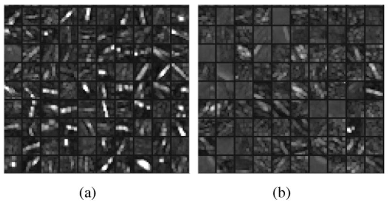
(a) Examples of feature maps obtained from 100 BAC samples; (b) examples of feature maps obtained from 100 non-BAC samples. The feature maps are the output of the third max-pooling layer. For each sample, only the feature map with highest energy is selected for display.

For better visualization of the learnt features, we also show the feature maps obtained after the first, second, and fourth max-pooling layers. The results are shown in Figures S3-S5 in Supplementary Materials.

V. conclusion

We have investigated the feasibility of building an automated system for BAC detection and calcification estimation in mammograms as possible risk markers for coronary artery disease. For this purpose, we first formulated the problem as a two-class classification problem. We considered a pixel-wise, patch-based procedure for BAC detection and applied a twelve-layer CNN to discriminate BAC pixels from non-BAC pixels. For a pixel under consideration, the input of the CNN is an image patch of size 95 × 95 centered on it. To compare the performance of the proposed approach to human performance, we conducted a two-round reader study. In the experiments, the performance was evaluated by both FROC analysis and calcium mass quantification analysis on a set of 840 FFDM images from 210 cases. The FROC analysis shows that the proposed approach obtains FPs of 0.4762 cm² with a TP rate of 60%, comparable to the performance of at least one of the readers. The calcium mass quantification analysis shows that the calcium mass inferred from the BAC detections is close to the ground-truth calcium mass; the linear regression analysis between them yields a coefficient of determination of 96.24%. Thus, while larger-scale studies are required to further refine and assess the approach, the results indicate that it brings automated BAC detection much closer to clinical translation.

References

- 1.Wenger NK. Psychosocial Stress and Cardiovascular Disease in Women. Springer; 2015. Coronary heart disease in women: evolution of our knowledge; pp. 13–25. [Google Scholar]
- 2.Mozaffarian D, Benjamin AS, Emelia J, Go, Arnett DK, et al. Heart disease and stroke statistics–2016 update: A report from the American Heart Association. Circulation. 2016;134(14):e38–360. doi: 10.1161/CIR.0000000000000350. [DOI] [PubMed] [Google Scholar]
- 3.Iribarren C, Go AS, Tolstykh I, Sidney S, Johnston SC, Spring DB. Breast vascular calcification and risk of coronary heart disease, stroke, and heart failure. Journal of Women's Health. 2004;13(4):381–389. doi: 10.1089/154099904323087060. [DOI] [PubMed] [Google Scholar]
- 4.Ferreira EMF, Szejnfeld J, Faintuch S. Correlation between intramammary arterial calcifications and CAD. Academic radiology. 2007;14(2):144–150. doi: 10.1016/j.acra.2006.10.017. [DOI] [PubMed] [Google Scholar]
- 5.Pecchi A, Rossi R, Coppi F, Ligabue G, Modena M, Romagnoli R. Association of breast arterial calcifications detected by mammography and coronary artery calcifications quantified by multislice CT in a population of post-menopausal women. La Radiologia Medica. 2003;106(4):305–312. [PubMed] [Google Scholar]
- 6.Matsumura ME, Maksimik C, Martinez MW, Weiss M, Newcomb J, Harris K, Rossi MA, et al. Breast artery calcium noted on screening mammography is predictive of high risk coronary calcium in asymptomatic women: a case control study. VASA Zeitschrift fur Gefasskrankheiten. 2013;42:429–433. doi: 10.1024/0301-1526/a000312. [DOI] [PubMed] [Google Scholar]
- 7.Maas AH, van der Schouw YT, Atsma F, Beijerinck D, Deurenberg JJ, Willem PTM, van der Graaf Y. Breast arterial calcifications are correlated with subsequent development of coronary artery calcifications, but their aetiology is predominantly different. European Journal of Radiology. 2007;63(3):396–400. doi: 10.1016/j.ejrad.2007.02.009. [DOI] [PubMed] [Google Scholar]
- 8.Ge J, Chan HP, Sahiner B, Zhou C, Helvie MA, Wei J, Hadjiiski LM, Zhang Y, Wu YT, Shi J. Medical Imaging. International Society for Optics and Photonics; 2008. Automated detection of breast vascular calcification on full-field digital mammograms; pp. 691 517–691 517. [Google Scholar]
- 9.Society AC. Cancer facts and figures 2016. 2016 [Google Scholar]
- 10.FDA approves first 3-D mammography imaging system. [accessed: 2016-09-18]; http://www.fda.gov/NewsEvents/Newsroom/PressAnnouncements/ucm243072.htm.
- 11.Molloi S, Mehraien T, Iribarren C, Smith C, Ducote JL, Feig SA. Reproducibility of breast arterial calcium mass quantification using digital mammography. Academic Radiology. 2009;16(3):275–282. doi: 10.1016/j.acra.2008.08.011. [DOI] [PMC free article] [PubMed] [Google Scholar]
- 12.Molloi S, Xu T, Ducote J, Iribarren C. Quantification of breast arterial calcification using full field digital mammography. Medical Physics. 2008;35(4):1428–1439. doi: 10.1118/1.2868756. [DOI] [PMC free article] [PubMed] [Google Scholar]
- 13.Cox J, Simpson W, Walshaw D. An interesting byproduct of screening: assessing the effect of hrt on arterial calcification in the female breast. Journal of Medical Screening. 2002;9(1):38–39. doi: 10.1136/jms.9.1.38. [DOI] [PubMed] [Google Scholar]
- 14.Rotter MA, Schnatz PF, Currier AA, Jr, O'Sullivan DM. Breast arterial calcifications (BACs) found on screening mammography and their association with cardiovascular disease. Menopause. 2008;15(2):276–281. doi: 10.1097/gme.0b013e3181405d0a. [DOI] [PubMed] [Google Scholar]
- 15.Duhn V, D'Orsi ET, Johnson S, D'Orsi CJ, Adams AL, O'Neill WC. Breast arterial calcification: a marker of medial vascular calcification in chronic kidney disease. Clinical Journal of the American Society of Nephrology. 2011;6(2):377–382. doi: 10.2215/CJN.07190810. [DOI] [PMC free article] [PubMed] [Google Scholar]
- 16.Reddy J, Bilezikian JP, Smith SJ, Mosca L. Reduced bone mineral density is associated with breast arterial calcification. The Journal of Clinical Endocrinology & Metabolism. 2008;93(1):208–211. doi: 10.1210/jc.2007-0693. [DOI] [PMC free article] [PubMed] [Google Scholar]
- 17.Kemmeren JM, Beijerinck D, Van Noord P, Banga JD, Deurenberg J, Pameijer FA, Van der Graaf Y. Breast arterial calcifications: association with diabetes mellitus and cardiovascular mortality. work in progress. Radiology. 1996;201(1):75–78. doi: 10.1148/radiology.201.1.8816524. [DOI] [PubMed] [Google Scholar]
- 18.Çetin M, Çetin R, Tamer N, Kelekçi S. Breast arterial calcifications associated with diabetes and hypertension. Journal of diabetes and its complications. 2004;18(6):363–366. doi: 10.1016/j.jdiacomp.2004.04.004. [DOI] [PubMed] [Google Scholar]
- 19.Cheng JZ, Cole EB, Pisano ED, Shen D. International Conference on Information Processing in Medical Imaging. Springer; 2009. Detection of arterial calcification in mammograms by random walks; pp. 713–724. [DOI] [PubMed] [Google Scholar]
- 20.Cheng JZ, Chen CM, Shen D. 2012 9th IEEE International Symposium on Biomedical Imaging (ISBI) IEEE; 2012. Identification of breast vascular calcium deposition in digital mam-mography by linear structure analysis; pp. 126–129. [Google Scholar]
- 21.Cheng JZ, Chen CM, Cole EB, Pisano ED, Shen D. Automated delineation of calcified vessels in mammography by tracking with uncertainty and graphical linking techniques. IEEE Transactions on Medical Imaging. 2012;31(11):2143–2155. doi: 10.1109/TMI.2012.2215880. [DOI] [PubMed] [Google Scholar]
- 22.Mordang JJ, Gubern-Mérida A, den Heeten G, Karssemeijer N. Reducing false positives of microcal-cification detection systems by removal of breast arterial calcifications. Medical physics. 2016;43(4):1676–1687. doi: 10.1118/1.4943376. [DOI] [PubMed] [Google Scholar]
- 23.Schmidhuber J. Deep learning in neural networks: An overview. Neural Networks. 2015;61:85–117. doi: 10.1016/j.neunet.2014.09.003. [DOI] [PubMed] [Google Scholar]
- 24.Krizhevsky A, Sutskever I, Hinton GE. Imagenet classification with deep convolutional neural networks. in Advances in neural information processing systems. 2012:1097–1105. [Google Scholar]
- 25.Szegedy C, Liu W, Jia Y, Sermanet P, Reed S, Anguelov D, Erhan D, Vanhoucke V, Rabinovich A. Going deeper with convolutions. Proceedings of the IEEE Conference on Computer Vision and Pattern Recognition. 2015:1–9. [Google Scholar]
- 26.Srivastava RK, Greff K, Schmidhuber J. Training very deep networks. Advances in Neural Information Processing Systems. 2015:2368–2376. [Google Scholar]
- 27.He K, Zhang X, Ren S, Sun J. Deep residual learning for image recognition. arXiv preprint arXiv:1512.03385. 2015 [Google Scholar]
- 28.Graves A, Mohamed Ar, Hinton G. Acoustics, Speech and Signal Processing (ICASSP), 2013 IEEE International Conference on. IEEE; 2013. Speech recognition with deep recurrent neural networks; pp. 6645–6649. [Google Scholar]
- 29.Baldi P, Sadowski P, Whiteson D. Searching for exotic particles in high-energy physics with deep learning. Nature Communications. 2014;5 doi: 10.1038/ncomms5308. [DOI] [PubMed] [Google Scholar]
- 30.Sadowski P, Collado J, Whiteson D, Baldi P. Deep learning, dark knowledge, and dark matter. Journal of Machine Learning Research, Workshop and Conference Proceedings. 2015;42:81–97. [Google Scholar]
- 31.Kayala MA, Azencott CA, Chen JH, Baldi P. Learning to predict chemical reactions. Journal of chemical information and modeling. 2011;51(9):2209–2222. doi: 10.1021/ci200207y. [DOI] [PMC free article] [PubMed] [Google Scholar]
- 32.Kayala MA, Baldi P. Reactionpredictor: Prediction of complex chemical reactions at the mechanistic level using machine learning. Journal of chemical information and modeling. 2012;52(10):2526–2540. doi: 10.1021/ci3003039. [DOI] [PubMed] [Google Scholar]
- 33.Lusci A, Pollastri G, Baldi P. Deep architectures and deep learning in chemoinformatics: the prediction of aqueous solubility for drug-like molecules. Journal of chemical information and modeling. 2013;53(7):1563–1575. doi: 10.1021/ci400187y. [DOI] [PMC free article] [PubMed] [Google Scholar]
- 34.Di Lena P, Nagata K, Baldi P. Deep architectures for protein contact map prediction. Bioinformatics. 2012;28(19):2449–2457. doi: 10.1093/bioinformatics/bts475. [DOI] [PMC free article] [PubMed] [Google Scholar]
- 35.Baldi P, Pollastri G. The principled design of large-scale recursive neural network architectures–DAG-RNNs and the protein structure prediction problem. Journal of Machine Learning Research. 2003;4(Sep):575–602. [Google Scholar]
- 36.Zhou J, Troyanskaya OG. Predicting effects of noncoding variants with deep learning-based sequence model. Nature methods. 2015;12(10):931–934. doi: 10.1038/nmeth.3547. [DOI] [PMC free article] [PubMed] [Google Scholar]
- 37.Cun YL, Boser B, Denker J, Henderson D, Howard R, Hubbard W, Jackel L. Handwritten digit recognition with a back-propagation network. In: Touretzky D, editor. Advances in Neural Information Processing Systems. San Mateo, CA: Morgan Kaufmann; 1990. pp. 396–404. [Google Scholar]
- 38.Baldi P, Chauvin Y. Neural networks for fingerprint recognition. Neural Computation. 1993;5(3):402–418. [Google Scholar]
- 39.Cireş D, Giusti A, Gambardella LM, Schmidhuber J. Deep neural networks segment neuronal membranes in electron microscopy images. Advances in neural information processing systems. 2012:2843–2851. [Google Scholar]
- 40.Roth HR, Yao J, Lu L, Stieger J, Burns JE, Summers RM. Recent Advances in Computational Methods and Clinical Applications for Spine Imaging. Springer; 2015. Detection of sclerotic spine metastases via random aggregation of deep convolutional neural network classifications; pp. 3–12. [Google Scholar]
- 41.Shen W, Zhou M, Yang F, Yang C, Tian J. International Conference on Information Processing in Medical Imaging. Springer; 2015. Multi- scale convolutional neural networks for lung nodule classification; pp. 588–599. [DOI] [PubMed] [Google Scholar]
- 42.Wang D, Khosla A, Gargeya R, Irshad H, Beck AH. Deep learning for identifying metastatic breast cancer. arXiv preprint arXiv:1606.05718. 2016 [Google Scholar]
- 43.Farabet C, Couprie C, Najman L, LeCun Y. Learning hierarchical features for scene labeling. IEEE transactions on pattern analysis and machine intelligence. 2013;35(8):1915–1929. doi: 10.1109/TPAMI.2012.231. [DOI] [PubMed] [Google Scholar]
- 44.Sermanet P, Eigen D, Zhang X, Mathieu M, Fergus R, LeCun Y. Overfeat: Integrated recognition, localization and detection using convolutional networks. arXiv preprint arXiv:1312.6229. 2013 [Google Scholar]
- 45.Ioffe S, Szegedy C. Batch normalization: Accelerating deep network training by reducing internal covariate shift. arXiv preprint arXiv:1502.03167. 2015 [Google Scholar]
- 46.Maas AL, Hannun AY, Ng AY. Rectifier nonlinearities improve neural network acoustic models. Proceedings of the 30th Internatinal Conference on Machine Learning. 2013;30(1) [Google Scholar]
- 47.Srivastava N, Hinton GE, Krizhevsky A, Sutskever I, Salakhutdinov R. Dropout: a simple way to prevent neural networks from overfitting. Journal of Machine Learning Research. 2014;15(1):1929–1958. [Google Scholar]
- 48.Baldi P, Sadowski P. The dropout learning algorithm. Artificial intelligence. 2014;210:78–122. doi: 10.1016/j.artint.2014.02.004. [DOI] [PMC free article] [PubMed] [Google Scholar]
- 49.Zhang TY, Suen CY. A fast parallel algorithm for thinning digital patterns. Communications of the ACM. 1984;27(3):236–239. [Google Scholar]
- 50.Burgess A. On the noise variance of a digital mam-mography system. Medical Physics. 2004;31(7):1987–1995. doi: 10.1118/1.1758791. [DOI] [PubMed] [Google Scholar]
- 51.Bottou L. Neural Networks: Tricks of the Trade. Springer; 2012. Stochastic gradient descent tricks; pp. 421–436. [Google Scholar]
- 52.Chatfield K, Simonyan K, Vedaldi A, Zisserman A. Return of the devil in the details: Delving deep into convolutional nets. arXiv preprint arXiv:1405.3531. 2014 [Google Scholar]
- 53.Wang J, Nishikawa RM, Yang Y. Improving the accuracy in detection of clustered microcalcifications with a context-sensitive classification model. Medical physics. 2016;43(1):159–170. doi: 10.1118/1.4938059. [DOI] [PMC free article] [PubMed] [Google Scholar]
Associated Data
This section collects any data citations, data availability statements, or supplementary materials included in this article.