Pixel-based meshfree modelling of skeletal muscles

Abstract

This paper introduces the meshfree Reproducing Kernel Particle Method (RKPM) for 3D image-based modeling of skeletal muscles. This approach allows for construction of simulation model based on pixel data obtained from medical images. The material properties and muscle fiber direction obtained from Diffusion Tensor Imaging (DTI) are input at each pixel point. The reproducing kernel (RK) approximation allows a representation of material heterogeneity with smooth transition. A multiphase multichannel level set based segmentation framework is adopted for individual muscle segmentation using Magnetic Resonance Images (MRI) and DTI. The application of the proposed methods for modeling the human lower leg is demonstrated.

1. Introduction

In the conventional Finite Element (FE) approach, the meshes need to be conformed to muscle geometry, which increases the complexity of mesh construction. Generally muscles have a complex architecture and poorly built meshes can easily lead to significant errors in FE analysis due to mesh distortion. Abrupt changes of topology in the muscle cross sections could also result in failure in FE mesh generation. Additionally, muscle material is anisotropic in nature due to the presence of muscle fibers. In FE modeling, one way to introduce the anisotropy is to approximate the fiber directions by interpolating from some pre-defined templates as described in (Blemker & Delp, 2005). The fiber directions obtained in this way could generate noticeable discretization errors in the simulation models. In this work, we develop an image based meshfree modeling technique based on a Reproducing Kernel Particle Method (RKPM) (Liu, et al., 1995; Chen, et al., 1996). The fiber direction obtained from Diffusion Tensor Imaging (DTI) data (Bihan, et al., 2001; Sinha & Yao, 2002) and the material properties are defined at pixel points and are directly used as input into meshfree modeling. Since no mesh is required in meshfree methods, the complexity related to meshing in finite element method is avoided. The Reproducing Kernel (RK) approximation also allows for a smooth transition of material properties at the interfaces between different materials in the muscle, which is required in the context of biological materials where the material interfaces do not exhibit sharp discontinuities. The skeletal muscle is represented as a nearly incompressible hyperelastic material (Chi, et al., 2010). RKPM has been used to simulate extremely large deformation of rubber like hyperelastic material (Chen, et al., 1996; Chen, et al., 1997).

Additionally, in this paper we propose a method for the segmentation of individual muscles which have different fiber orientation. Automatically segmenting individual muscle components from Magnetic Resonance Images (MRI) poses a difficult problem as the boundaries between different muscles are not clearly distinguishable. The most popular method used for this segmentation is to introduce prior knowledge into the segmentation process through registration (Maintz & Viergever, 1998) of images or statistical learning techniques (Baudin, et al., 2012; Baudin, et al., 2012; Prescott, et al., 2011; Neji, et al., 2008). The idea proposed in this work is to use the MRI intensities in combination with the muscle fiber direction obtained from DTI, to segment individual muscles. A combined multiphase multichannel method of segmentation is used to implement this idea (Vese & Chan, 2002; Chan, et al., 2000). The multichannel framework incorporates the MRI and fiber direction data in different channels, and a multiphase framework is required to segment multiple connected regions in an image.

The remaining sections of the paper are arranged as follows. Section 2 gives the review of the RK approximation and the smooth transition between heterogeneous materials using RK approximation is demonstrated. In Section 3, the variational formulation of hyperelasticity discretized by RKPM is introduced. The details of the proposed DTI enhanced multiphase-multichannel level set segmentation of muscles and full RKPM model construction from images are given in Section 4. Section 5 demonstrates the application of the proposed meshfree pixel based method to modeling of skeletal muscles. Concluding remarks are given in Section 6.

2. Reproducing Kernel (RK) Approximation

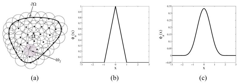
In meshfree modeling, the problem domain is discretized with a set of arbitrarily distributed points (nodes) as shown in Figure 1(a). Each point I is associated with an open cover ω_I which defines the locality of the approximation defined on ω_I. In the present modeling, the pixel coordinates of the geometry are obtained from the images and are used as nodes for discretizing the domain for the meshfree modeling. The RK shape functions are constructed based on a set of points and are used to approximate the displacement field governed by the equilibrium equation or equation of motion of a solid (Liu, et al., 1995; Chen, et al., 1996). The derivation of the RK shape function is given in the following paragraphs.

Figure 1.

(a) Domain discretization in meshfree modeling. Here Ω represents the domain and ∂Ω represents the boundary of the domain. Sample kernel functions: (b) Tent function (c) Cubic B-Spline function

Let α = α₁α₂...α_d represent the multi-dimensional index notation, where d is the spatial dimension and |α| = α₁ + α₂ +... +α_d. The following notations are used:

$${\mathbf{x}}^{\alpha }={\mathbf{x}}_1^{{\alpha }_1}{\mathbf{x}}_2^{{\alpha }_2}\dots {\mathbf{x}}_d^{{\alpha }_d},{(\mathbf{x}-{\mathbf{x}}_I)}^{\alpha }={({\mathbf{x}}_1-{\mathbf{x}}_{1I})}^{{\alpha }_1}{({\mathbf{x}}_2-{\mathbf{x}}_{2I})}^{{\alpha }_2}\dots {({\mathbf{x}}_d-{\mathbf{x}}_{dI})}^{{\alpha }_d}$$ (1)

Consider a domain Ω in d dimensional space R^d which is discretized by a set of NP nodes given by ${\left\{{\mathbf{x}}_I\mid {\mathbf{x}}_I\in \mathrm{\Omega }\right\}}_{I=1}^{NP}$. The RK approximation of a function u is given by:

$$u^h(\mathbf{x})=\sum _{I=1}^{NP}{\mathrm{\Psi }}_I(\mathbf{x})d_I$$ (2)

where Ψ_I(x) is the RK approximation function (also called the RK shape function) of node I, d_I is the coefficient at node I and u^h (x) is the approximated function. The RK shape function is expressed as:

$${\mathrm{\Psi }}_I(\mathbf{x})=C(\mathbf{x};\mathbf{x}-{\mathbf{x}}_I){\varphi }_a(\mathbf{x}-{\mathbf{x}}_I)$$ (3)

where ϕ_a (x–x_I) is a kernel function which determines the locality of the approximation by its compact support measured by ‘a’ and the smoothness of the approximation. Examples of kernel functions are given in Figure 1(b) and (c) where the tent function is C₀ continuous and the cubic B-spline function is C₂ continuous.

The term (x;x – x_I) C is a correction function expressed as:

$$C(\mathbf{x};\mathbf{x}-{\mathbf{x}}_I)=\sum _{\mid \alpha \mid =0}^n{(\mathbf{x}-{\mathbf{x}}_I)}^{\alpha }{\mathbf{b}}_{\alpha }(\mathbf{x})={\mathbf{H}}^T(\mathbf{x}-{\mathbf{x}}_I)\mathbf{b}(\mathbf{x})\text{in}{R}^d$$ (4)

where n is the order of the basis functions, ${\mathbf{H}}^T(\mathbf{x}-{\mathbf{x}}_I)={\{{(\mathbf{x}-{\mathbf{x}}_I)}^{\alpha }\}}_{\mid \alpha \mid =0}^n$ is a vector containing all the monomial basis functions, and b_α (x) is an unknown vector which is determined by the following n^th order consistency conditions:

$$\sum _{I=1}^{NP}{\mathrm{\Psi }}_I(\mathbf{x}){\mathbf{x}}_I^{\alpha }={\mathbf{x}}^{\alpha };\mid \alpha \mid =0,\dots ,n$$ (5)

The above equation is equivalent to ${\displaystyle \sum _{I=1}^{NP}}{\mathrm{\Psi }}_I(\mathbf{x})\mathbf{H}(\mathbf{x}-{\mathbf{x}}_I)=\mathbf{H}(0)$ and the unknown coefficient vector is obtained as b(x) =M⁻¹(x) H(0) where M is called the moment matrix, given by:

$$\mathbf{M}(\mathbf{x})=\sum _{I=1}^{NP}\mathbf{H}(\mathbf{x}-{\mathbf{x}}_I){\mathbf{H}}^T(\mathbf{x}-{\mathbf{x}}_I){\varphi }_a(\mathbf{x}-{\mathbf{x}}_I)$$ (6)

The correction function introduced in the reproducing kernel approximation enables it to exactly satisfy the reproducing conditions everywhere in the domain and on the boundary in the discrete form (Chen, et al., 1998). Finally, the RK shape function can be re-written as:

$${\mathrm{\Psi }}_I(\mathbf{x})={\mathbf{H}}^T(\mathbf{0}){\mathbf{M}}^{-1}(\mathbf{x})\mathbf{H}(\mathbf{x}-{\mathbf{x}}_I){\varphi }_a(\mathbf{x}-{\mathbf{x}}_I)$$ (7)

Examples of 1D and 2D RK shape functions are given in Figure 2. From the process of constructing the reproducing kernel shape function, it can be seen that the order of completeness of the approximation is determined by the order of consistency, that is, the order of basis functions ‘n’. The convergence behavior of the RK shape function in approximating a sinusoidal function u(x) = sin(x), x∈[0, 10] is illustrated in Figure 3. Here, the error is computed based on the following L₂ error measure:

$$\mathit{error}={\left[\underset{\mathrm{\Omega }}{\int }{(u^h-u)}^{2}d\mathrm{\Omega }\right]}^{\frac{1}{2}}$$ (8)

where u^h is the approximated function, u is the exact function and the problem domain Ω is [0, 10] in this example. It can be seen in Figure 3 that the RK shape function using second order basis shows higher convergence rate, when compared to the case using first order basis. It is also shown that while the smoothness of the kernel function does not affect the convergence rate, the accuracy for RK shape function increases by using smoother kernel function.

Figure 2.

(a) One dimensional reproducing kernel shape function centered at node x = 5.0, (b) Two dimensional reproducing kernel shape function centered at node (x, y) = (5.0, 5.0)

Figure 3.

Convergence behavior for approximating sinusoidal function with h the nodal spacing. (a) Basis order is n = 1, and (b) Basis order is n = 2. The respective rates of convergence are given on the plot.

It is noted that the RK approximation functions do not possess Kronecker Delta property, i.e Ψ_I (x_J) ≠ δ_IJ. Due to this condition, numerous methods have been proposed to impose the essential boundary conditions, including the Lagrange multiplier method (Belytschko, et al., 1994; Chen, et al., 1997), transformation method (Chen & Wang, 2000; Chen, et al., 1996), Nitsche’s method and penalty method (Sonia & Huerta, 2004). In this work, the penalty method is used for imposing the essential boundary conditions.

It has been shown in many studies (Tidball, 1984) that the change of material properties from skeletal muscle to tendon is a smooth transition. Heterogeneous material modeling using FE representation results in jumps in material properties at the material interfaces, and the computed stresses and strains are also discontinuous across the element boundaries. On the contrary, in the proposed meshfree RKPM analysis the material properties are assigned to the nodes and the material properties transition represented by the smooth RK approximation can be made with the desired smooth transition, which avoids the abrupt jumps of stresses and strains. This RK representation of the smooth transition in material properties is illustrated in the following example. Consider a region x∈[0, 10] with the interface at x = 5 between two materials, where the Young’s moduli (E) are given by: E = 30 for x∈[0, 5) and E =5 for x∈[5, 10]. As can be seen in Figure 4, finite element approximation exhibits a sharp discontinuity at x = 5.0 while the RK approximation shows smooth transition in representing the material property transition across the material interface by choosing appropriate kernel function support size ‘a’ in the RK approximation.

Figure 4.

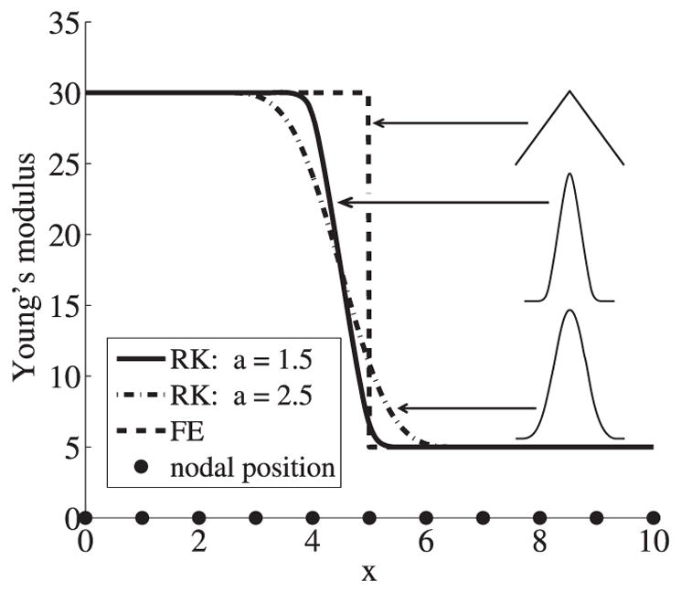
1D comparison of RK and FE approximations of the Young’s modulus. Cubic B-Spline kernel function and linear basis are used.

3. Meshfree RKPM Formulation for Hyperelasticity

In this section, a 3D RKPM formulation is introduced to solve the hyperelastic problem, in which the penalty method is used to impose the essential boundary conditions. The formulation is based on the total Lagrangian framework, where the implementation is carried out in the reference or undeformed configuration. Let the problem domain in the undeformed configuration be denoted by Ω_X, with the corresponding essential boundary and natural boundary denoted by $\partial {\mathrm{\Omega }}_X^g$ and $\partial {\mathrm{\Omega }}_X^h$, respectively. The energy functional for this total Lagrangian formulation can be written as follows:

$$U={\int }_{{\mathrm{\Omega }}_X}W(\mathbf{u})d\mathrm{\Omega }-{\int }_{{\mathrm{\Omega }}_X}{u}_i{b}_{i}d\mathrm{\Omega }-{\int }_{\partial {\mathrm{\Omega }}_X^h}{u}_i{h}_{i}d\mathrm{\Gamma }+\frac{\beta }{2}{\int }_{\partial {\mathrm{\Omega }}_X^g}(u_i-g_i)(u_i-g_i)d\mathrm{\Gamma }$$ (9)

where W(u) is the strain energy density function, b is the body force per unit undeformed volume, h is the prescribed surface force per unit undeformed area on the natural boundary $\partial {\mathrm{\Omega }}_X^h$, β is the penalty number and g is the prescribed displacement on the essential boundary $\partial {\mathrm{\Omega }}_X^g$. The stationary condition is obtained by taking variation of equation (9), which yields:

$${\int }_{{\mathrm{\Omega }}_X}\delta F_{ij}{P}_{ji}d\mathrm{\Omega }+\beta {\int }_{\partial {\mathrm{\Omega }}_X^g}\delta u_i{u}_{i}d\mathrm{\Gamma }={\int }_{{\mathrm{\Omega }}_X}\delta u_i{b}_{i}d\mathrm{\Omega }+{\int }_{\partial {\mathrm{\Omega }}_X^h}\delta u_i{h}_{i}d\mathrm{\Gamma }+\beta {\int }_{\partial {\mathrm{\Omega }}_X^g}\delta u_i{g}_{i}d\mathrm{\Gamma }$$ (10)

where F is the deformation gradient and P is the first Piola-Kirchhoff stress. Due to the geometric and material nonlinearities, Newton’s method is used to solve the nonlinear equations and the linearization of equation (10) is required. Let n and ν denote the current load step counter and iteration step counter, respectively, the linearized equation is given by:

$${\int }_{{\mathrm{\Omega }}_X}\delta F_{ij}{(C_{\mathit{ijkl}})}_{n+1}^{\nu }\mathrm{\Delta }{F}_{kl}d\mathrm{\Omega }+\beta {\int }_{\partial {\mathrm{\Omega }}_X^g}\delta u_i\mathrm{\Delta }{u}_{i}d\mathrm{\Gamma }={\int }_{{\mathrm{\Omega }}_X}\delta u_i{(b_i)}_{n+1}d\mathrm{\Omega }+{\int }_{\partial {\mathrm{\Omega }}_X^h}\delta u_i{(h_i)}_{n+1}d\mathrm{\Gamma }+\beta {\int }_{\partial {\mathrm{\Omega }}_X^g}\delta u_i[{(g_i)}_{n+1}-{(u_i)}_{n+1}^{\nu }]d\mathrm{\Gamma }-{\int }_{{\mathrm{\Omega }}_X}\delta F_{ij}{(P_{ji})}_{n+1}^{\nu }d\mathrm{\Omega }$$ (11)

where C_ijkl is the first elasticity tensor. The displacement vector, its variation and the incremental displacement vector are approximated by the RK shape functions as follows:

$$\mathbf{u}=\sum _{I=1}^{NP}{\mathbf{N}}_I{\mathbf{d}}_I,\delta \mathbf{u}=\sum _{I=1}^{NP}{\mathbf{N}}_I\delta {\mathbf{d}}_I,\mathrm{\Delta }\mathbf{u}=\sum _{I=1}^{NP}{\mathbf{N}}_I\mathrm{\Delta }{\mathbf{d}}_I$$ (12)

where

$${\mathbf{u}}^T=[\begin{array}{ccc}{u}_1& u_2& u_3\end{array}],{\mathbf{d}}_I^T=[\begin{array}{ccc}{d}_{1I}& d_{2I}& d_{3I}\end{array}],{\mathbf{N}}_I=\left[\begin{array}{ccc}{\mathrm{\Psi }}_I& 0& 0\\ 0& {\mathrm{\Psi }}_I& 0\\ 0& 0& {\mathrm{\Psi }}_I\end{array}\right]$$ (13)

Here Ψ_I is the Lagrangian RK shape function defined as:

$${\mathrm{\Psi }}_I(\mathbf{X})=C(\mathbf{X};\mathbf{X}-{\mathbf{X}}_I){\varphi }_a^X(\mathbf{X}-{\mathbf{X}}_I)$$ (14)

and the kernel ${\varphi }_a^X$ is called the ‘material kernel’ given by:

$${\varphi }_a^X(\mathbf{X}-{\mathbf{X}}_I)={\varphi }_a^X\left(\frac{\Vert \mathbf{X}-{\mathbf{X}}_I\Vert }{a}\right)$$ (15)

As shown in the above equation, the material kernel is defined using the distance measured by the material coordinate in the reference configuration. The support of the material kernel function covers the same set of nodes throughout the history of deformation and hence the associated shape function is called the ‘Lagrangian’ shape function. An illustration of the material kernel function that deforms with material deformation is given in Figure 5.

Figure 5.

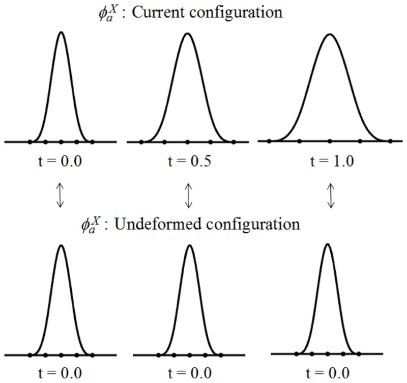
Material kernel function (cubic B-spline)

The incremental deformation gradient in vector form is given by:

$$\mathrm{\Delta }\mathbf{F}=\sum _I{\mathbf{B}}_I\mathrm{\Delta }{\mathbf{d}}_I$$ (16)

where

$$\begin{array}{ll}{\mathbf{F}}^T\hfill & =[\begin{array}{lllllllll}{F}_{11}\hfill & F_{22}\hfill & F_{33}\hfill & F_{12}\hfill & F_{21}\hfill & F_{13}\hfill & F_{31}\hfill & F_{23}\hfill & F_{32}\hfill \end{array}]\hfill \\ {\mathbf{B}}_I^T\hfill & =\left[\begin{array}{ccccccccc}{\mathrm{\Psi }}_{I,1}& 0& 0& {\mathrm{\Psi }}_{I,2}& 0& {\mathrm{\Psi }}_{I,3}& 0& 0& 0\\ 0& {\mathrm{\Psi }}_{I,2}& 0& 0& {\mathrm{\Psi }}_{I,1}& 0& 0& {\mathrm{\Psi }}_{I,3}& 0\\ 0& 0& {\mathrm{\Psi }}_{I,3}& 0& 0& 0& {\mathrm{\Psi }}_{I,1}& 0& {\mathrm{\Psi }}_{I,2}\end{array}\right]\hfill \end{array}$$ (17)

Here, Ψ_I,j = ∂Ψ_I / ∂X_j. Taking the material derivative of the Lagrangian RK shape function is straightforward.

By introducing the RK approximation for displacements given in equation (12) and the deformation gradient given in equation (16) into the linearized equation (11), the following matrix equation is obtained:

$${\mathbf{K}}_{IJ}\mathrm{\Delta }{\mathbf{d}}_J={\mathbf{f}}_I^{\text{ext}}-{\mathbf{f}}_I^{int}$$ (18)

where I, J = 1,…,NP. The dimension of stiffness K_IJ is 3×3 and that of Δd_J is 3×1 and

$$\begin{array}{l}{\mathbf{K}}_{IJ}={\int }_{{\mathrm{\Omega }}_X}{\mathbf{B}}_I^T\mathbf{C}{\mathbf{B}}_{J}d\mathrm{\Omega }+\beta {\int }_{\partial {\mathrm{\Omega }}_X^g}{\mathbf{N}}_I^T{\mathbf{N}}_{J}d\mathrm{\Gamma }\\ {\mathbf{f}}_I^{int}={\int }_{{\mathrm{\Omega }}_X}{\mathbf{B}}_I^T\mathbf{P}d\mathrm{\Omega }\\ {\mathbf{f}}_I^{\text{ext}}={\int }_{{\mathrm{\Omega }}_X}{\mathbf{N}}_I^T\mathbf{b}d\mathrm{\Omega }+{\int }_{\partial {\mathrm{\Omega }}_X^h}{\mathbf{N}}_I^T\mathbf{h}d\mathrm{\Gamma }+\beta {\int }_{\partial {\mathrm{\Omega }}_X^g}{\mathbf{N}}_I^T(\mathbf{g}-{\mathbf{u}}_{n+1}^{\nu })d\mathrm{\Gamma }\end{array}$$ (19)

and

$$\begin{array}{l}\mathbf{P}={[\begin{array}{lllllllll}{P}_{11}\hfill & P_{22}\hfill & P_{33}\hfill & P_{12}\hfill & P_{21}\hfill & P_{13}\hfill & P_{31}\hfill & P_{23}\hfill & P_{32}\hfill \end{array}]}^T\\ \mathbf{b}={[\begin{array}{lll}{b}_1\hfill & b_2\hfill & b_3\hfill \end{array}]}^T,\mathbf{h}={[\begin{array}{lll}{h}_1\hfill & h_2\hfill & h_3\hfill \end{array}]}^T\end{array}$$ (20)

where C is a 9×9 matrix and each element is given by C_AB = ∂²W/∂F_A∂F_B.

The method of Stabilized Conforming Nodal Integration (SCNI) (Chen, et al., 2001; Chen, et al., 2002; Puso, et al., 2008) is used for integrating the discrete equations in (18) where a smoothed derivative of the approximation function is used in conjunction with a nodal integration in equation (17) to achieve computational efficiency and accuracy. SCNI ensures a quadratic rate of convergence in Galerkin meshfree approximation of the equilibrium equation, and it achieves greater computational efficiency and accuracy for the meshfree method compared to conventional Gauss quadrature rules.

4. Model Construction from Images

4.1 Segmentation of individual muscles

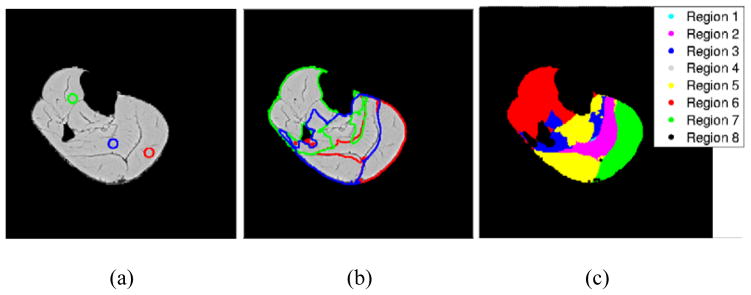
For individual muscle segmentation, the idea proposed in this work is to use the muscle fiber direction which is obtained from DTI data at each pixel point, along with the MRI as input for segmentation using a combined multiphase multichannel level set based segmentation method. This method works efficiently for segmenting adjacent muscles which have different fiber orientation. In DT imaging a 3×3 diffusion tensor is obtained at each voxel (volumetric pixel) which gives the diffusion in each direction in vivo by quantifying the random movement of water molecules in the muscle. The principal eigen vectors and eigen values of the diffusion tensor give the main directions of diffusion and the associated diffusivities, respectively (Bihan, et al., 2001). The eigen vector corresponding to the maximum eigenvalue is called the lead Eigen Vector (EV). This lead Eigen Vector of diffusion tensor at each pixel point is assumed to give the muscle fiber direction at that point. Here, the method is implemented to segment the muscles from the MRI and DTI data of the human lower leg. This EV data, which consists of a vector at each pixel point, is obtained in 3 images where each image gives one of the vector components. For the purpose of segmentation, the EV data is scaled to be at the similar level of the MRI intensities. Each of the images, that is, MRI, e₁, e₂ and e₃ components of the EV data are taken as 4 channels for segmentation. As the final segmentation has 7 major muscles to be identified in the image, at least 3 level set functions (ϕ’s ) should be used for segmentation, since ‘K’ level set functions can segment up to 2^K regions in an image (Vese & Chan, 2002). The functional for the 3 level sets, 4 channels segmentation is given by (Vese & Chan, 2002; Chan, et al., 2000):

$$\mathrm{\Pi }(c_p^i,{\varphi }_1,{\varphi }_2,{\varphi }_3)=\sum _{K=1}^3{\mu }_K\underset{\mathrm{\Omega }}{\int }\delta ({\varphi }_K)|\nabla {\varphi }_K|\mathrm{d}\mathbf{x}+\sum _{p=1}^8\left(\underset{{\mathrm{\Omega }}_p}{\int }\frac{1}{4}\sum _{i=1}^4\left({\lambda }_p^i{(u_o^i(\mathbf{x})-c_p^i)}^2\right)\mathrm{d}\mathbf{x}\right)$$ (21)

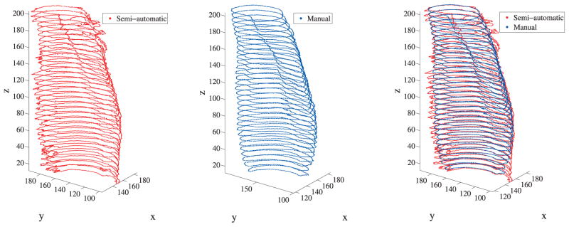
where ϕ_K denotes the K^th level set function, $u_o^i(\mathbf{x})$ denotes the pixel intensity in the i^th channel at point x, p denotes the number of regions that can be segmented, μ_K denotes the weight for the length regularization term for the zeroth isocontour of the level set functions, and $c_p^i$ denotes the unknown constants which represents the mean value of intensity in the region Ω_p of the i^th channel. A μ value of either 1 or 100 was used for all level set functions, to obtain the required segmentation for a particular image slice. The expressions for $c_p^i$ can be obtained by minimizing equation (21) with respect to each $c_p^i$ keeping all other variables constant. The 3 Euler-Lagrange equations for curve evolution can be obtained by minimizing the above functional with respect to ϕ₁,ϕ₂ and ϕ₃, respectively, keeping $c_p^i$ constant. These are solved using a semi-implicit finite difference scheme. The pixels belonging to a particular region in the image can be obtained according to the sign of all the level set functions in that region. For this muscle segmentation, the important parameter to consider in the formulation given in equation (21) is the λ terms which are the weights for the forcing term. If the value of λ is decreased, it allows for slightly more variance of intensities in the region to be segmented and vice versa. This parameter allows for taking into account the slight variation of muscle fiber directions in each individual muscle. Figure 6 shows the segmentation result for one of the MRI slices by taking λ = 0.02 in all channels and regions, and μ =1 was taken for all level set functions. As can been seen in this segmentation result, the Medial Gastrocnemius (MG) muscle (green color) has been segmented very well. The MG muscle is segmented using the proposed method from 33 images and compared with manual segmentation as shown in Figure 7. Muscles with different fiber orientations need to be segmented to separate groups so that different anisotropic material properties can be specified in the computational model.

Figure 6.

Multiphase multichannel segmentation of MRI and EV data (a) Initial contours of the 3 level set functions (b) Final contours obtained from segmentation (c) Final segmented regions

Figure 7.

Comparison of semi-automatic and manual segmentations of the medial gastrocnemius muscle of human lower leg. The units of x,y and z coordinates are in pixel coordinates where 1 pixel = 0.078125 cm.

4.2 Full model construction

The following methodology is developed for constructing the full model of the human lower leg from medical images. The geometry is extracted through segmentation of the anatomical MRI. Muscle, Intra-Muscular Connective Tissue (IMCT), fat (including both intra-muscular fat (IMAT) and subcutaneous fat) are the materials included in the construction of the model. The IMCT and IMAT are segmented independently using a separate specialized sequences of MR images. The Chan-Vese level set segmentation method (Chan & Vese, 2001) is used for extracting boundaries of the bones and the outer boundary of the lower leg from each MRI as shown in Figure 8(a)–(c). The interior points of boundary contours are obtained as shown in Figure 8(d). The segmented IMAT and IMCT points (shown in Figure 8(e)) are subtracted from these interior points to obtain an image (say image 1). The points which have EV data are chosen as the muscle points in image 1 and the remaining interior points are assigned as fat since they constitute the outer subcutaneous fat layer. The final image obtained with all the different material points labeled is shown in Figure 9(a). A coarse image was generated for computational efficiency, by creating a coarse set of points with larger spacing between the pixels. The nodal spacing in the fine model is 1 pixel, whereas in the coarse model it is taken as 2 pixels. The muscle, fat and IMCT of the coarse image can be obtained by sorting common points between the coarse and the fine images for each slice. The coarser image generated is shown in Figure 9(b). This procedure is repeated for every image (slice) and the 3D pixel based model is constructed by stacking the slices as shown in Figure 9(c).

Figure 8.

(a) Initial contour (b) Chan Vese segmentation result (c) Outer contours and bone contours obtained from segmentation (d) Interior points (e) Segmented intra-muscular fat and IMCT points overlapped on MRI

Figure 9.

(a) Fine model (b) Coarse model (c) 3D model constructed from 25 images of the coarse model, has 73,659 nodes. On the plot, the numbers 1, 2 and 3 indicate the transverse, coronal and sagittal planes, respectively. The units of x,y and z coordinates are in pixel coordinates where 1 pixel = 0.078125 cm.

5. Pixel Based Meshfree Modeling of Skeletal Muscle

A transversely isotropic hyperelastic model is employed to represent the mechanical behavior of skeletal muscle. The strain energy density function for the muscle is decoupled into isotropic and anisotropic parts as defined below:

$$W_{\text{muscle}}=W_{\text{matrix}}({\overline{I}}_1,{\overline{I}}_2,J)+W_{\text{fiber}}(\widehat{\lambda })$$ (22)

where W_matrix is the strain energy stored within the isotropic muscle matrix, W_fiber is the strain energy stored within muscle fiber and this introduces anisotropy to the model. ${\overline{I}}_1=I_1{I}_3^{-1/3},{\overline{I}}_2=I_1{I}_3^{-2/3}$, where I₁, I₂, and I₃ are the three invariants of right Cauchy-Green strain tensor C, $\widehat{\lambda }=\sqrt{\widehat{\mathbf{N}}·\overline{\mathbf{C}}·\widehat{\mathbf{N}}}$ is the stretch ratio along the fiber direction N̂, and C̄ = J^−2/3C. A quadratic polynomial type strain energy density function for W_matrix as employed in (Chi, et al., 2010) is used in this study:

$$W_{\mathit{matrix}}=\sum _{i+j=1}^2{C}_{ij}{({\overline{I}}_1-3)}^i{({\overline{I}}_2-3)}^j+\frac{K}{2}{(J-1)}^2$$ (23)

The fiber stress is related to the energy density function W_fiber as follows:

$$\widehat{\lambda }\frac{\partial W_{\text{fiber}}}{\partial \widehat{\lambda }}={\sigma }_{max}\frac{\widehat{\lambda }}{{\widehat{\lambda }}_0}(\alpha f_{\text{active}}+f_{\text{passive}})$$ (24)

where λ̂₀ is the stretch ratio at optimal length, σ_max is the maximum isometric stress, α is the activation factor which represents the level of activation in the muscle fiber, f_active and f_passive are the normalized active and passive fiber forces, respectively, given by (Chi, et al., 2010):

$$\{\begin{array}{ll}{f}_{\text{passive}}=0\hfill & \text{for}{\lambda }^{\ast }\le 1\hfill \\ f_{\text{passive}}={\gamma }_1({\mathrm{e}}^{{\gamma }_2({\lambda }^{\ast }-1)}-1)\hfill & \text{for}1<{\lambda }^{\ast }\le 1.4\hfill \\ f_{\text{passive}}=({\gamma }_1{\gamma }_2{\mathrm{e}}^{0.4{\gamma }_2}){\lambda }^{\ast }+{\gamma }_1({\mathrm{e}}^{0.4{\gamma }_2}-1)\hfill & \text{for}{\lambda }^{\ast }>1.4\hfill \end{array}$$ (25)

$$\{\begin{array}{ll}{f}_{\text{active}}=9{({\lambda }^{\ast }-0.4)}^2\hfill & \text{for}{\lambda }^{\ast }\le 0.6\hfill \\ f_{\text{active}}=1-4{(1-{\lambda }^{\ast })}^2\hfill & \text{for}0.6<{\lambda }^{\ast }\le 1.4\hfill \\ f_{\text{active}}=9{({\lambda }^{\ast }-1.6)}^2\hfill & \text{for}{\lambda }^{\ast }>1.4\hfill \end{array}$$ (26)

where λ^* = λ̂/λ̂₀ is the normalized stretch ratio, and γ₁ = 0.05 and γ₂ = 6.6.

Connective tissue and fat are modeled by an isotropic cubic hyperelastic model with the strain energy density function defined as (Chi, et al., 2010):

$$W=C_{10}({\overline{I}}_1-3)+C_{20}{({\overline{I}}_1-3)}^2+C_{30}{({\overline{I}}_1-3)}^3+\frac{K}{2}{(J-1)}^2$$ (27)

The calibrated values of material constants for muscle and connective tissue are adopted from (Chi, et al., 2010). The material constants for the fat are 10 times softer than those of the connective tissue. The material constants used in this work are summarized in Table 1 for connective tissue and fat, and in Table 2 for muscle.

Table 1.

Material constants for connective tissue and fat (N/cm²)

	C10	C20	C30	K
Connective tissue	30	80	800	50,000
Fat	3	8	80	5000

Table 2.

Material constants for muscle matrix (N/cm²)

	C10	C01	C20	C02	C11	K
Muscle	6.43	−3.8	0.94	0.0005	−0.0043	5000

Hodgson et al. (Hodgson, et al., 2012) demonstrated how anisotropy in the material model affects the deformation in a muscle with simplified geometry. The anisotropy in the proposed simulation model includes the transversely isotropic hyperelastic material model which accounts for the presence of muscle fibers, as well as the irregular distribution of tissues like connective tissue, which yield an overall anisotropic property in the simulation model. The complexity in microstructures (IMCT and IMAT) also accounts for the model anisotropy.

As can be seen in the full lower leg model given in Figure 9(c), the pixel resolution in the longitudinal z-direction is lower than the resolution in the transverse xy-direction. This is due to the fact that in the MRI acquisition, the scanning in the vertical direction is only taken at certain intervals. In the meshfree modeling, this is taken into account by using a suitable support size in the RK approximation function, which is adjusted according to the nodal spacing in different directions in the model. This discretization is also consistent with the deformation of muscle, where the spatial variations of stress and strain fields in the longitudinal direction are much less than those in the transverse direction. In this work, the RK support size in the longitudial direction is about 3 times of that in the transverse direction. In all the following examples, the reproducing kernel approximation functions are constructed using a cubic spline kernel function and linear basis. A normalized support size of a/h=1.65 is used, where a is the support size of the kernel function and h is the nodal spacing.

Example 1: Comparison of meshfree and finite element modeling of tendon

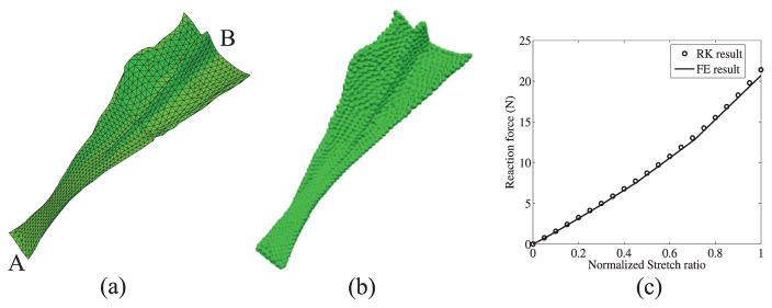
To show the accuracy of the RKPM method, a manually segmented tendon model whose structure is relatively regular (and thus FEM discretization is possible), is modeled using both RKPM and finite element method. The discretization of the model using finite element and meshfree nodes are shown in Figure 10(a) and Figure 10(b), respectively. The length of the tendon is about 19 cm. The bottom surface A of the tendon is fixed in all directions and the top surface B is stretched by 2 cm in the direction along the axial direction of the tendon, (see Figure 10(a)). The tendon is modeled with the cubic hyperelastic model described in equation (27) for which the material parameters are given in Table 1. The comparison of the reaction forces generated at the fixed end using meshfree and finite element methods are shown in Figure 10(c), which show very good agreement.

Figure 10.

3D model of tendon (a) Finite element discretization (b) Meshfree discretization (c) Comparison of the reaction forces generated at the fixed end, using Finite Element (FE) and meshfree (RK) methods

Example 2: Numerical analysis of isometric contraction of the lower leg using RKPM

In this example, isometric contraction of the 3D muscle model of the lower leg shown in Figure 9(c), which is constructed from slices of the coarse image (Figure 9(b)), is simulated using the RKPM formulation. Isometric contraction is achieved by fixing the top and bottom boundaries. For the points near the interior bone boundaries, the displacements in the cross-sectional plane are fixed but are free to move along the longitudinal direction of the muscle. The activation factor α of the muscle material is linearly increased from 0 to 0.95. In our simulation, all muscle points are activated simultaneously. The generated force due to muscle contraction is calculated at the fixed end. The reaction force generated at different levels of muscle activation is shown in Figure 11. A convergence study is performed to ensure that the discretization resolution of muscle model (Figure 9(c)) is sufficient for desired accuracy. A refined RKPM model is generated from finer cross-sectional image as shown in Figure 9(a). The spacing in the longitudinal direction (vertical z-direction) is not refined due to the limitation in the image acquisition. This is also justified due to the fact that the spatial variations in the stress and strain fields in the longitudinal direction are much smaller than those in the transverse direction. The force generation results obtained from the coarse and refined models are shown in Figure 11, which confirm convergence of the RKPM solution.

Figure 11.

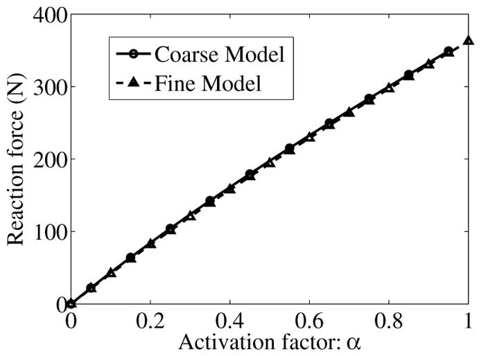
Reaction force generated at different levels of muscle activation predicted by the coarse and refined models

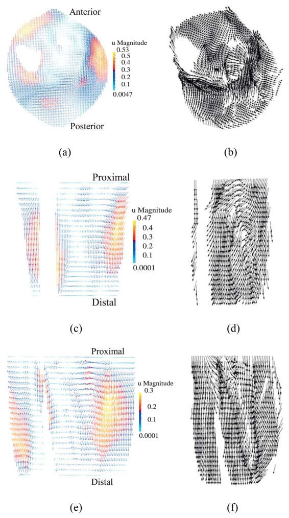
In Figure 12(a)–(f) the nodal displacement vectors are plotted on sample planes (transverse, coronal, sagittal) on the reference (undeformed) configuration. The muscle fiber directions in the undeformed configuration are also plotted for comparison. The results show that while in certain areas the nodal displacement vectors are approximately in the direction of the muscle fibers, no particular correlation between them is observed. As can be seen in the sagittal cross-section in Figure 12(e), the points near the posterior region displace downwards towards the distal end and the points near the anterior region move upwards toward the proximal end due to muscle contraction. Figure 13 shows the maximum principal Cauchy stress in the full model and on sample planes at the final configuration. It is important to note that the stress fields shown in Figure 13 are calculated using the RK approximation functions which are continuous in its first order derivatives. Thus, the computed stress field is continuous, in contrast to finite element method which yields discontinuous stress field across element boundaries.

Figure 12.

Displacement vectors (left) and corresponding fiber directions (right) plotted on reference configuration on (a)–(b) transverse plane at z = 5 cm; (c)–(d) coronal plane at y = 10.1 cm; (e)–(f) sagittal plane at x = 10 cm. (units of u magnitude: cm). Note: The fiber directions are plotted only at the muscle points, whereas displacements are shown at all material points.

Figure 13.

Distribution of the maximum principal Cauchy stress (N/cm²) at the final deformed configuration (a) full model (b) at transverse planes z = 5.0 cm (c) at coronal plane y = 10.1 cm

Example 3: Comparison of force production in young and old muscles

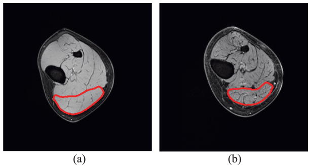
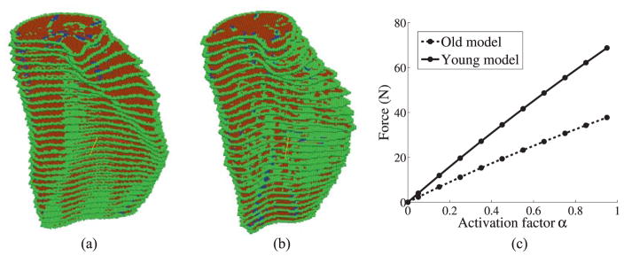
Two MG models from young and old subjects were selected to investigate the effect of aging on force generation. Sample MRI slices of these young and old subjects are given in Figure 14(a) and (b), respectively, which clearly show the increased amount of connective tissue in the older subject. The MG muscle is outlined in red in these figures. The segmented MG models of the young and old subjects with the same axial length are shown in Figure 15(a) and (b), respectively. The MG is surrounded by an outer layer of connective tissue which forms the aponeurosis. The volumes of the different material components in the young and the old models are given in Table 3. It should be noted that IMCT here does not include the aponeurosis.

Figure 14.

Connective tissue visualization from MRI of (a) young and (b) old models. The medial gastrocnemius muscle is outlined in red.

Figure 15.

(a) MG muscle of the young model (b) MG muscle of the old model. Here green points are the connective tissue, red points are muscle and blue points are fat (IMAT) (c) Comparison of force generation versus activation level between young and old models

Table 3.

Example 2: Young vs Old Model Results comparison

	Young model	Old model	Old normalized by Young
Muscle(cm3)	98.93	61.89	62.5%
IMAT(cm3)	2.83	6.15	217.3%
IMCT(cm3)	20.86	29.15	139.7%
Fmax (N)	68.76	37.74	54.8%

In the numerical simulation, both ends of the muscle are fixed and the activation of the muscle is increased to simulate isometric contraction. The muscle force activation characteristics for both the young and the old muscles are taken to be the same. The force generation at maximum activation shows that the younger model generates much bigger force than the older model (Figure 15(c)). The effective force generated per unit total volume (including the outer layer of connective tissue) for the younger model is 0.430 N/cm³ and for the old model is 0.294 N/cm³. This shows that the amount of non-contractile tissue strongly affects the force production. It is worth noting that the muscle volume of the older model is about 37% smaller than that of the younger model but the force generation in the older model drops by around 45% compared to the young model. There is a disproportionate decrease in force production due to the decrease in muscle volume. These results from numerical modeling support the hypothesis that the amount of connective tissue in the muscle affects the force production considerably (Csapo, et al., 2014).

6. Conclusions

In this work, an image based meshfree RKPM computational framework is developed for skeletal muscle modeling. A method for RKPM simulation model construction with different material components is developed by extracting pixel data from medical images. The pixel points from these images can be directly used as nodes for domain discretization in the meshfree modeling, and the fiber direction obtained from the DTI data is input directly at each pixel point, without the need for additional processing or interpolation. The employed reproducing kernel approximation can represent the smooth transition of material properties in heterogeneous materials. The variation of material properties in the transition zone can be controlled by adjusting the support size of the kernel function in the RK approximation. These properties of image based meshfree methods render it suitable for subject specific modeling.

A multiphase multichannel level set approach for segmenting individual muscles using both MRI and DTI data is also proposed. Using this method, adjacent muscles in the image which have different fiber orientations can be segmented. The multichannel method enables the incorporation of MRI and EV data in different channels for segmentation, and a multiphase framework is required to segment connected regions in an image. Numerical examples are given to demonstrate the effectiveness of the proposed image based meshfree method for modeling the mechanical behavior of skeletal muscles. A preliminary study of force production between young and old skeletal muscles having different amounts of non-contractile tissue volumes is performed. A disproportionate decrease in force production is observed due to the decrease in muscle volume between the young and the old MG muscles.

References

- Baudin P-Y, Azzabou N, Carlier PG, Paragios N. Automatic Skeletal Muscle Segmentation Through Random Walks and Graph-Based Seed Placement. International Symposium on Biomedical Imaging. 2012;2012:1036–1039. [Google Scholar]
- Baudin P-Y, Azzabou N, Carlier PG, Paragios N. Prior Knowledge, Random Walks and Human Skeletal Muscle Segmentation. In: Ayache N, et al., editors. MICCAI 2012, Part I, LNCS 7510. Volume Springer-Verlag; Berlin Heidelberg: 2012. pp. 569–576. [DOI] [PubMed] [Google Scholar]
- Belytschko T, Lu Y, Gu L. Element Free Galerkin Methods. International Journal for Numerical Methods in Engineering. 1994;37:229–256. [Google Scholar]
- Bihan DL, et al. Diffusion Tensor Imaging: Concepts and Applications. Journal of Magnetic Resonance Imaging. 2001;13:534–546. doi: 10.1002/jmri.1076. [DOI] [PubMed] [Google Scholar]
- Blemker SS, Delp SL. Three-dimensional representation of complex muscle architectures and geometries. Annals of Biomedical Engineering. 2005;33(5):661–673. doi: 10.1007/s10439-005-1433-7. [DOI] [PubMed] [Google Scholar]
- Chan TF, Sandberg BY, Vese LA. Active Contours without Edges for Vector-Valued Images. Journal of Visual Communication and Image Representation. 2000;11:130–141. [Google Scholar]
- Chan TF, Vese LA. Active Contours without edges. IEEE Transactions on Image Processing. 2001;10(2):266–277. doi: 10.1109/83.902291. [DOI] [PubMed] [Google Scholar]
- Chen JS, Pan C, Roque MOL, Wang HP. A Lagrangian reproducing kernel particle method for metal forming analysis. Computational mechanics. 1998;22(3):298–307. [Google Scholar]
- Chen JS, Pan C, Wu CT. Large deformation analysis of rubber based on a reproducing kernel particle method. Computational Mechanics. 1997:211–227. [Google Scholar]
- Chen JS, Pan C, Wu CT, Liu WK. Reproducing kernel particle methods for large deformation analysis of non-linear structures. Computer Methods in Applied Mechanics and Engineering. 1996:195–227. [Google Scholar]
- Chen JS, Wang H-P. New boundary condition treatments in meshfree computation of contact problems. Computer methods in applied mechanics and engineering. 2000;187:441–468. [Google Scholar]
- Chen JS, Wu CT, Yoon S, You Y. A stabilized conforming nodal integration for Galerkin mesh-free methods. International Journal for Numerical Methods in Engineering. 2001:435–466. [Google Scholar]
- Chen JS, Yoon S, Wu CT. Non-linear version of stabilized conforming nodal integration for Galerkin mesh-free methods. International Journal for Numerical Methods in Engineering. 2002:2587–2615. [Google Scholar]
- Chi SW, et al. Finite element modeling reveals complex strain mechanics in the aponeuroses of contracting skeletal muscle. Journal of biomechanics. 2010;43(7):1243–1250. doi: 10.1016/j.jbiomech.2010.01.005. [DOI] [PMC free article] [PubMed] [Google Scholar]
- Csapo R, et al. Age-associated differences in triceps surae muscle composition and strength – an MRI-based cross-sectional comparison of contractile, adipose and connective tissue. BMC Musculoskeletal Disorders. 2014;15:1–11. doi: 10.1186/1471-2474-15-209. [DOI] [PMC free article] [PubMed] [Google Scholar]
- Hodgson JA, et al. Finite element modeling of passive material influence on the deformation and force output of skeletal muscle. Journal of the Mechanical Behavior of BioMedical Materials. 2012;9:163–183. doi: 10.1016/j.jmbbm.2012.01.010. [DOI] [PMC free article] [PubMed] [Google Scholar]
- Liu WK, Jun S, Zhang YF. Reproducing kernel particle methods. International journal for numerical methods in fluids. 1995;20(8–9):1081–1106. [Google Scholar]
- Maintz JBA, Viergever MA. A survey of medical image registration. Medical Image Analysis. 1998;2(1):1–36. doi: 10.1016/s1361-8415(01)80026-8. [DOI] [PubMed] [Google Scholar]
- Neji R, et al. Support Vector Driven Markov Random Fields Towards DTI Segmentation of the Human Skeletal Muscle. International Symposium on Biomedical Imaging. 2008:923–926. [Google Scholar]
- Prescott JW, et al. Anatomically Anchored Template-Based Level Set Segmentation: Application to Quadriceps Muscles in MR Images from the Osteoarthritis Initiative. Journal of Digital Imaging. 2011;24(1):28–43. doi: 10.1007/s10278-009-9260-2. [DOI] [PMC free article] [PubMed] [Google Scholar]
- Puso MA, Chen J-S, Zywicz E, Elmer W. Meshfree and Finite Element Nodal Integration methods. International Journal for Numerical Methods in Engineering. 2008;74:416–446. [Google Scholar]
- Sinha U, Yao L. In vivo diffusion tensor imaging of human calf muscle. Journal of Magnetic Resonance Imaging. 2002:87–95. doi: 10.1002/jmri.10035. [DOI] [PubMed] [Google Scholar]
- Sonia F-M, Huerta A. Imposing essential boundary conditions in meshfree methods. Computer methods in applied mechanics and engineering. 2004;193:1257–1275. [Google Scholar]
- Tidball JG. Myotendinous junction: morphological changes and mechanical failure associated with muscle cell atrophy. Experimental and molecular pathology. 1984;40(1):1–12. doi: 10.1016/0014-4800(84)90060-1. [DOI] [PubMed] [Google Scholar]
- Vese LA, Chan TF. A Multiphase Level set Framework for Image segmentation using the Mumford and Shah model. International Journal of Computer Vision. 2002;50(3):271–293. [Google Scholar]