Quantitative Image Reconstruction for Total-Body PET Imaging Using the 2-meter Long EXPLORER Scanner

Abstract

The EXPLORER project aims to build a 2-meter long total-body PET scanner, which will provide extremely high sensitivity for imaging the entire human body. It will possess a range of capabilities currently unavailable to state-of-the-art clinical PET scanners with a limited axial field-of-view. The huge number of lines-of-response (LORs) of the EXPLORER poses a challenge to the data handling and image reconstruction. The objective of this study is to develop a quantitative image reconstruction method for the EXPLORER and compare its performance with current whole-body scanners. Fully 3D image reconstruction was performed using time-of-flight list-mode data with parallel computation. To recover the resolution loss caused by the parallax error between crystal pairs at a large axial ring difference or transaxial radial offset, we applied an image domain resolution model estimated from point source data. To evaluate the image quality, we conducted computer simulations using the SimSET Monte-Carlo toolkit and XCAT 2.0 anthropomorphic phantom to mimic a 20-minute whole-body PET scan with an injection of 25 MBq ¹⁸F-FDG. We compare the performance of the EXPLORER with a current clinical scanner that has an axial FOV of 22 cm. The comparison results demonstrated superior image quality from the EXPLORER with a 6.9-fold reduction in noise standard deviation comparing with multi-bed imaging using the clinical scanner.

1. Introduction

Positron emission tomography (PET) is a molecular imaging technique that has been widely used in oncology, neurology, and cardiology. It also has applications in clinical research and drug development. Current clinical PET scanners have an axial field-of-view (FOV) of 15~25 cm in length, which offers limited body coverage and relatively low photon detection efficiency (Badawi et al 2000, Cherry 2006). As a result, a typical clinical ¹⁸F-FDG PET scan requires an injected activity of about 200~500 MBq (i.e. 5.4~13.5 mCi). To explore the maximum potential of PET, the EXPLORER consortium aims to build a 2-meter long total-body PET system (Badawi et al 2013, Cherry et al 2013) (Figure 1), called the EXPLORER (EXtreme Performance Long REsearch scanneR), which will provide massively increased sensitivity and possess a range of capabilities currently unavailable with existing scanners. The long axial coverage can yield a sensitivity gain of 30~40 times that of current scanners (Poon 2013). The high sensitivity can be used for high-throughput scans and offers the potential to perform a whole-body examination in a single breath-hold. The increased sensitivity will also allow imaging at very low radiation doses (down to an injected dose of ~10 MBq) (Zhang et al 2014a, Zhang et al 2014b). It will allow application of PET to pediatric and adolescent populations, studying and monitoring chronic disease, and much more. Moreover we can conduct dynamic PET imaging with simultaneous total-body coverage as compared to the current multi-bed multi-pass imaging protocol with large temporal gaps (Karakatsanis et al 2013).

Figure 1.

Artistic illustration of the EXPLORER system.

Some work has been conducted to investigate the sensitivity and noise equivalent count rate (NECR) performance of long axial FOV PET scanners (Wong et al 2007, Couceiro et al 2007, Eriksson et al 2007, Eriksson et al 2011, Crespo et al 2012, Poon et al 2012, Poon 2013, Isnaini et al 2014a, Isnaini et al 2014b). Image quality and lesion detectability were also studied for performance evaluation between different scanner designs (Badawi et al 2013, Surti et al 2013, Surti et al 2015). Some demonstration scanners with an extended AFOV (50~70 cm) have been built and provide significant sensitivity, but achieved very limited improvement of performance due to the limitations in data acquisition electronics (Watanabe et al 2004, Conti et al 2006). To enlarge the axial FOV without increasing cost, the concept of open-gap PET was proposed and a prototype scanner has been built for pre-clinical research (Yoshida et al 2010, Yamaya et al 2011). However, this design provides no improvement in sensitivity and the reconstructed images may have artifacts due to incomplete sampling issues (Tashima et al 2014).

The EXPLORER consortium is now in the process of constructing the first 2-meter long PET scanner prototype, which is based on the detector technology from commercial PET scanners. It will have more than 400,000 crystals in total and form over 50 billion lines of response, which is about 100 times more than that of a current clinical PET scanner. Therefore, efficient data handling is very important. In this paper, we present a quantitative image reconstruction method for the EXPLORER and use Monte Carlo simulated data to evaluate the image quality.

2. Methods

2.1. The simulated EXPLORER scanner

The simulated EXPLORER system configuration and simulation parameters are listed in Table 1. The scanner consists of 36 axial block rings with an axial gap of 3.42 mm (one crystal pitch) between adjacent rings. Each ring has 48 51×51 mm² detector modules forming a ring of 800 mm in diameter. Each detector module consists of an array of 15×15 LSO crystals with a crystal pitch of 3.42 mm. The time-of-flight (TOF) resolution of 530 ps was chosen to mimic the timing performance in a Siemens Biograph mCT PET scanner.

Table 1.

System configuration of the simulated EXPLORER scanner

System parameters	Value
scintillator material	LSO
crystal size (mm)	3.34×3.34×20
crystal pitch (mm) (+80 μm reflector)	3.42
number of crystals per block detector	15×15
number of block detectors per ring	48
number of block rings	36
ring diameter (mm)	800
transaxial FOV (mm)	700
gap size between adjacent block rings (mm)	3.42 (one crystal pitch)
axial FOV (mm)	1966
energy resolution	13%
energy window (keV)	[435, 650]
TOF resolution (ps)	530
timing bin size (ps)	25
coincidence timing window (ns)	±5.5

2.2. Image Reconstruction and Resolution modeling

Statistically-based iterative image reconstruction methods can provide improved image quality by using accurate statistical and physical models of the PET imaging process. In general PET data y ∈ ℛ^M×1can be modeled as a collection of independent Poisson random variables with the expectation, ȳ ∈ ℛ^M×1, related to the unknown radiotracer distribution x ∈ ℛ^N×1 through an affine transformation with a system matrix P ∈ ℛ^M×N (Qi et al 2006)

$$\overline{\mathit{y}}=\mathit{E}[\mathit{y}\mid \mathit{x}]=\mathit{Px}+\overline{\mathit{s}}+\overline{\mathit{r}}$$ (1)

The (i, j)th element of P, p_ij, models the probability of a radioactive decay from the jth image voxel being detected by the ith LOR. s̄ and r̄ denote the expectations of scatters and randoms, respectively.

Since the EXPLORER scanner has more than 50 billion LORs and records time-of-flight information, list-mode data format is preferred for efficient data processing. An additional consideration for EXPLORER is that the axial resolution can be degraded by the parallax effect between crystal pairs with a large ring difference as illustrated in Figure 2. A more oblique LOR (red color) penetrates more adjacent crystals than a LOR of less ring difference (blue color). It is similar to the radial blurring effect at large radial offset in a transaxial plane. Figure 2 (lower right) shows reconstructions of a simulated point source without any resolution modeling with a maximum block-ring difference (MBRD) of ~30, 110 and 200 cm, respectively. Clearly we observe worse axial resolution with longer tails as we increase the maximum ring difference, although the resolution degradation effect is less dramatic because the effect of oblique LORs is mitigated by direct LORs passing through the same point. Therefore, it is necessary to model the resolution loss in both radial and axial directions in the list-mode image reconstruction. We adopt an image domain resolution model by factoring the system matrix P into three major components (Zhou and Qi 2014):

$$\mathit{P}=\mathit{DGR}$$ (2)

where D = diag {n} is a diagonal matrix containing normalization and attenuation factors, G is a simplified geometric projection matrix calculated by a ray-tracing algorithm (Siddon et al 1985) with a TOF kernel, and R is an image blurring matrix which models the resolution degradation effects, such as the positron range, photon acollinearity, and detector responses including inter-crystal penetration and inter-crystal scatter effects.

Figure 2.

Axial resolution blurring effect occurred at center of the FOV for different maximum ring difference. The point source images were reconstructed using 30 iterations of a LM TOF ML-EM algorithm.

For simplicity, the image domain point spread functions (PSFs) are considered to be separable in the transaxial plane and axial direction, i.e., the PSF at each point satisfies

$$\text{PSF}(x,y,z)={\text{PSF}}_t(x,y){\text{PSF}}_a(z).$$ (3)

Note that both the transaxial PSF and axial PSF are spatially variant. However, we assumed that the PSF_t is rotationally invariant, i.e., two points with the same radial distance to the FOV center share the same transaxial PSF after rotation, and the PSF_a(z) is kept invariant within the same axial plane. Therefore, we only need to estimate the transaxial PSF along a radial line and the axial PSF along the scanner z-axis. We simulated 101 point sources along the radial direction and 265 point sources along the axial direction (¹⁸F source in water for modeling the positron range) with a spacing of 3.42 mm which is equal to the voxel size used in reconstructions. We used a list-mode TOF ML-EM (LM TOF ML-EM) algorithm to reconstruct the 366 point sources individually, and then estimated the separable blurring kernels in the whole FOV by fitting a 2D Gaussian mixture model (two Gaussians) in the transaxial plane and 1D Gaussian model in the axial direction, respectively. Figure 3 shows examples of the estimated blurring kernels and the FWHM (Full Width at Half Maximum) and FWTM (Full Width at Tenth Maximum) values are listed in Table 2 for selected radial locations. The total storage size of the PSFs is less than 50 MB for the EXPLORER.

Figure 3.

Examples of the estimated image domain resolution kernels. (a) 2D transaxial radial blurring kernel at 17.2 cm radial offset; (b) 1D axial blurring kernels from the center to 90 cm axial offset (MBRD=20).

Table 2.

FWHM and FWTM of transaxial blurring kernels.

Radial Offset	0 cm	10 cm	20 cm	30 cm
Radial FWHM	3.0 mm	3.9 mm	5.6 mm	6.8 mm
Radial FWTM	5.4 mm	7.1 mm	10.2 mm	12.3 mm
Tangential FWHM	3.0 mm	3.4 mm	3.4 mm	3.5 mm
Tangential FWTM	5.4 mm	6.1 mm	6.3 mm	6.3 mm

2.3. Normalization

Normalization is required in reconstruction to compensate for the variations in detector efficiencies and geometric factors that are not modeled in the geometric projection matrix. To obtain the normalization factors, we simulated a uniform cylinder with a dimension of 70 cm in diameter and 200 cm in length using SimSET. To reduce the simulation time, we used a 1×1×1 voxel for the emission map and attenuation map and set the parameter of ‘Target Cylinder’ to the above-mentioned dimensions to constrain the source inside the cylinder. ¹⁸F source in ‘air’ was used. After ~2800 cpu-hours of simulation time, a total of 12.8 billion true coincidence events were acquired. To increase the statistics of the normalization factor in each individual LOR, we took advantage of the geometric symmetry in the scanner. For each LOR, there is a 48-fold rotational symmetry in the transaxial plane by rotating the LOR over M × 360/48 degrees (M = 1,..,47, and 48 is the number of transaxial blocks) and another 2-fold reflection symmetry for the LORs belongs to the same block pair in the transaxial plane. In addition, there is a N(= 36 – BRD)-fold parallel symmetry in the axial direction, where BRD is the block ring difference ranging from 0 to 35. Therefore, the counting statistics of each LOR can be increased by 96 × N-fold. Figure 4 shows an example of the LORs sharing the same normalization factor, where the red line represents the original LOR, the blue, green and purple ones represent the symmetric LORs. Figure 5(a) shows the original sinogram of the cylinder, which has no obvious pattern because of the low counts per pixel. Figure 5(b) shows the sinogram after averaging by both the axial and transaxial symmetries. The pronounced block pattern was caused by the inter-crystal scatters and the energy threshold, which effectively reduces the detection efficiency of edge crystals in a block. The final normalization factors were computed as the ratio between the averaged SimSET sinogram and the forward projection of the same cylinder using G.

Figure 4.

An illustration of LORs sharing the same normalization factors with the transaxial and axial symmetries. (a) The original LOR of the detected event (red solid line), 48-fold angular (blue dashed line) and 2-fold reflection (green dotted line) symmetries. (b) axial parallel symmetry with same ring difference (dashed lines).

Figure 5.

One transaxial sinogram of the simulated uniform cylinder for normalization (BRD=2). (a) The sinogram with axial symmetry only (34-fold). (b) The sinogram with both axial symmetry and transaxial symmetry (3,264-fold). The left figure aims to demonstrate the significant reduction in statistical uncertainty obtained by using the symmetry operations.

2.4. Scatter estimation and correction

Due to the long axial FOV of EXPLORER, photons may have longer paths through scattering material, resulting in greater opportunities for multiple scattering than may be seen in conventional PET scanners. To model multiple scatters, we used a Monte Carlo based scatter estimation in this study. We assume that the scatter sinogram is relatively smooth after proper correction by detector efficiencies. Therefore, we estimate the expectation of the scatter sinogram by histogramming the scatter events in Monte Carlo simulation by detector block pairs and also using a coarse TOF bin size (e.g. 225 ps here). This effectively increases the counts by 15⁴ × 225/25 ≈ 4.5 × 10⁵ fold, resulting in a nearly noise-free scatter sinogram. For the simulated EXPLORER with 36 block rings and 48 detector modules per ring, the storage size of the 5-D^‡ block-pair based scatter sinogram is 197 MB in floating point. In the list-mode image reconstruction, we computed the scatter mean for each event using a 5-D linear interpolation between the adjacent block-pairs and TOF bins, and then scaled to the timing bin (e.g. 25 ps here) for reconstruction.

2.5. Random estimation

For random correction, we use the following formula to calculate the mean random rate (cps) (Knoll 2000)

$$R_{ij}=2\tau S_i{S}_j$$ (4)

where τ is the coincidence timing window, and S_i and S_j are the singles rates of crystals i and j, respectively. For TOF data, the formula is changed to

$$R_{ij}^{\mathit{TOF}}={\tau }_{\mathit{\Delta }}{S}_i{S}_j$$ (5)

where τ_Δ is the TOF bin size (25 ps in our simulated study).

2.6. Evaluation study

To evaluate the system performance, we conducted computer simulations using the SimSET Monte-Carlo toolkit (Harrison et al 2006). We employed the XCAT 2.0 anthropomorphic adult male phantom (Segars et al 2010) (Figure 6) with a height of 178 cm in the simulation. To evaluate the capability of low dose imaging provided by EXPLORER, we modeled an injected activity of 25 MBq (~675 μCi), which is about 1/20^th of the standard dose administered in clinical PET scan protocols. To simulate a 20 minute ¹⁸F-FDG PET scan starting 60 minutes post-injection, different time-activity curves were generated for 14 major organs and tissues (Zhang et al 2014a). In addition, two spherical lesions of 10-mm in diameter were simulated inside of the liver and lung with a local contrast of 3.2 and 14.4, respectively.

Figure 6.

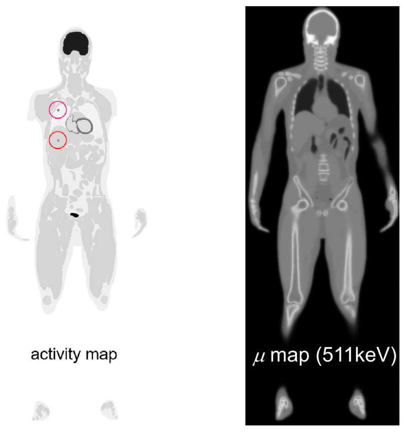
XCAT 2.0 phantom used for the total-body simulation. Two lesions were added in the right lung and liver (marked by red circles).

To generate random coincidences, we ran a separate SimSET simulation in the ‘SPECT’ mode and then doubled the event rates to get the coincidence singles rates for PET. The ¹⁷⁶Lu source in LSO cannot be simulated directly using SimSET. Instead we used a measured singles rate of 105 cps/cc (within the energy window of 435 to 650 keV) based on Siemens mCT block detectors. Therefore, the singles rate from LSO background is about 24 cps per crystal (volume of 0.23 cm³), which was added to the singles events from the object. Then we generated a Poisson random variable with the mean of R_ij = 2τS_iS_jΔT (Knoll 2000) to simulate random coincidences in each LOR, where ΔT is the scan duration. The maximum ring difference was set to 20 axial blocks (115 cm) to maximize the noise equivalent count rate (NECR) based previous studies (Poon et al 2012, Poon 2013). A constant coincidence timing window of τ = 5.5 ns was used to cover the entire FOV. In practice, a ring-difference dependent variable timing window can be used to reduce the number of random events, but the fraction of randoms within the FOV and the image quality will not be affected when TOF information is used.

Table 3 lists the three imaging protocols that were evaluated to compare the performance of the EXPLORER for low-dose static imaging with a clinical scanner. The first imaging protocol considered a 4 block-ring PET scanner at a single bed position that recorded data for 20 minutes over the liver region (4BR-single, Figure 7(a)). The second imaging protocol was a whole-body multi-bed scan using the 4 block-ring system (4BR-multi, Figure 7(b)). Each bed scan lasted 0.6 minutes and the total imaging time was also 20 minutes. This protocol is similar to whole-body imaging with continuous bed motion. The third imaging protocol was using the EXPLORER (36BR, Figure 7(c)) and also corresponded to a 20 minute scan. The first two sets of simulation data (4BR-single and 4BR-multi) were generated by sorting the events from the EXPLORER simulation with a maximum block-ring difference of 3 (MBRD=3), which mimics a current clinical scanner with an axial FOV of 22 cm. For each imaging scenario, we estimated the respective image domain resolution model using point source scans. Ten independent, identically distributed noisy realizations were generated for each protocol to estimate the uncertainty in the region of interest (ROI) quantification.

Table 3.

Comparison of the three scan protocols

Scan protocol	4BR single-bed	4BR multi-bed	36BR
# of block rings	4	4	36
# of crystal rings	60	60	540
# of bed positions	1	33	1
axial FOV	21.55 cm	197 cm	197 cm
# counts in total	80M (MBRD=3)	58M (MBRD=3)	3.17B (MBRD=20)
Total scan time	20 minutes	20 minutes	20 minutes

Figure 7.

Illustration of the three scan protocols. (a) 4BR single-bed torso scan; (b) 4BR multi-bed whole-body scan; (c) the EXPLORER total-body scan.

To evaluate the image quality, we calculate the contrast recovery coefficients (CRC) of the liver and lung lesions and the background variability (STD) from the reconstructed images. The true lesion masks were used as the lesion ROIs. The background ROIs were drawn in the liver and lung, respectively, excluding the lesion and boundary voxels. The CRC was calculated by

$$\text{CRC}(\%)=\frac{(\text{lesion}\text{mean})/(\text{background}\text{mean})-1}{\text{true}\text{contrast}-1}\times 100\%$$ (6)

and the STD was defined as the standard deviation of the voxel values inside the background ROI.

2.7. Computational time

The software of the 3D TOF list-mode OS-EM algorithm was coded in C++ and compiled using the GNU GCC (g++) compiler with the option ‘O3’ for optimization. Ten iterations and 10 subsets were used for all image reconstructions which is enough to achieve effective convergence (see results in the next section). The image dimension were 195 × 195 × 527 with a voxel size of 3.42 × 3.42 × 3.42 mm³. Processing 3.17 billion coincidences took 8.7 minutes per iteration (6.1 million events per second) on a computer with dual sixteen-core CPUs (Intel(R) Xeon(R) CPU E5-2683 v4 @ 2.1 GHz).

3. Results

3.1. Scatter estimation

We first plot in Figure 8(a) the numbers of detected true events and scattered events as a function of ring difference for the anthropomorphic phantom simulation. Clearly both numbers decrease rapidly with increasing ring difference due to the fact that there are fewer number of sinograms and stronger object attenuation at larger ring differences. The small peaks in the curves are caused by the axial gaps between block rings. Figure 8(b) shows a trend of increasing scatter fraction in individual sinograms as a function of the ring difference (red curve), but the overall scatter fraction in the fully 3D PET data remains relatively flat across all maximum ring differences (blue curve). The slight decrease in scatter fraction for ring difference less than 25 cm is because the anthropomorphic phantom is only 178 cm tall and does not cover the whole axial FOV of the scanner.

Figure 8.

(a) The numbers of trues (T) and scatters (S) in the direct/oblique sinograms as a function of ring difference. (b) Scatter fraction S/(S+T) in individual sinograms as a function of ring difference (red curve) and in all sinograms for a given maximum ring difference (blue curve).

Furthermore we examined the contributions of multiple scatters in the EXPLORER. Figure 9 plots the percentages of single scatters, double scatters, triple scatters and other scatters as a function of ring difference. Figure 10 shows the axially summed scatter sinograms. Here the double and triple scatters are defined by the total number of scattering interactions undergone by the two coincident photons inside the object. For example, a double scatter means either one photon is scattered twice or both photons are scattered once each. We can see that the fraction of multiple scatters increases as a function of ring difference with the percentage of single scatters decreasing from 85% in direct planes to 75% at the largest ring difference.

Figure 9.

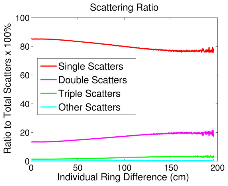
Fractions of single scatters and multiple scatters as a function of ring difference.

Figure 10.

Sinogram summed in the axial direction: (a) Single scatters (412 million); (b) double scatters (71 million); (c) triple scatters (8 million); (d) other scatters (0.74 million).

To verify the accuracy of the 5-D linear interpolation, we compared the axially summed scatter sinogram and estimated scatter mean from the 5-D interpolation in Figure 11. The difference sinogram between the estimated scatter mean and MC scatters is shown in Figure 11(c) and the profile comparison in Figure 11(d). It shows that the block-pair based average with 5-D interpolation provides a good estimate of the scatter distribution.

Figure 11.

Comparison of the reference scatter sinogram from Monte Carlo simulation and the block-pair averaged scatter mean sinogram summed in the axial direction. (a) The reference MC scatter sinogram (494 million); (b) the estimated scatter mean from 5D linear interpolation of block-pair sinogram; (c) the difference sinogram between (b) and (a); (d) profiles along the central row in (a) and (b).

3.2. Randoms estimation

Figure 12(a) shows the singles rate map from the SimSET simulation in combination with the LSO background, which represents S_i and S_j in equation (5). The horizontal and vertical axes correspond to the transaxial and axial crystal indices, respectively. Figure 12(b) shows the axial sum of the estimated mean of the random events, which is relatively uniform across the FOV. The total number of random events was 1.57 billion, among which 1.06 billion events (67.1% of the total randoms) contained at least one photon that originated from the Lu-176 background radiation.

Figure 12.

(a) Simulated singles rate map from the combination of the object and LSO background. The vertical axis represents 36 axial block rings and the horizontal axis represents 48 transaxial blocks/ring, with each block consisting of 15×15 crystals. (b) The axial sum of the random sinogram.

3.3. Image reconstruction

For the anthropomorphic phantom simulation, a total of 3.17 billion coincident events were recorded (MBRD=20), including 35.3% trues, 15.1% scatters and 49.6% randoms. We first compared our list-mode reconstruction with different levels of data correction: (1) Trues+Scatters+Randoms without any correction (T+S+R w/o c); (2) True events only with resolution modeling (T-only w/RM); (3) Trues+Scatters+Randoms with scatter and random correction but without resolution modeling (T+S+R w/sc+rc w/o RM); and 4) Trues+Scatters+Randoms with scatter and random correction and resolution modeling (T+S+R w/sc+rc+RM). Figure 13 and Figure 14 show the reconstruction results. We can see that with scatter correction, random correction and resolution modeling (T+S+R w/sc+rc+RM), the image quality is close to the result of the trues-only reconstruction (T-only w/RM) and more details in the lower spinal region can be seen compared with either no correction or partial correction. For quantitative comparison, Figure 15 compares the CRC vs. STD curves for the liver and lung lesions. The lowest curve in each group is from the reconstruction without any correction. The second lowest curve is the result with only scatter and random corrections. The two highest curves are obtained by using resolution modeling. The fact that the curve of T+S+R w/sc+rc+RM reaches almost the same CRC as that of the trues-only reconstruction indicates that the scatter and random corrections are fairly accurate.

Figure 13.

One realization showing reconstructed coronal and transaxial images with different levels of quantitative correction. Gaussian post-smoothing (σ = 0.6 pixel) was applied for better visualization.

Figure 14.

One realization showing reconstructed sagittal images with different levels of quantitative correction. Gaussian post-smoothing (σ = 0.6 pixel) was applied for better visualization.

Figure 15.

A comparison of CRC vs. background STD in the reconstructed images with different levels of quantitative correction. Top: the liver lesion; bottom: the lung lesion.

Figure 16 compares the reconstructed image of the EXPLORER with those from a 4-block-ring PET scanner for the imaging protocols listed in Table 3. Obviously, the best image quality was achieved by the EXPLORER. The 4BR-multi produced a very noisy image. The lesion in the liver is difficult to identify. Limiting the FOV of the 4BR to one bed position reduced the noise, but the image is still noisier than that obtained by the EXPLORER.

Figure 16.

Reconstructed images from three scan protocols. (a) 4BR single-bed scan; (b) 4BR multi-bed whole-body scan; (c) the EXPLORER total-body scan. Gaussian post-smoothing (σ = 0.6 pixel) was applied for better visualization.

Figure 17 compares the CRC-STD curves for the lesion in the liver (the lung lesion is outside the 4BR-single bed FOV). The error bars were estimated from the 10 realizations of each scan protocol. It is shown that with the proper resolution modeling, all three protocols achieved a similar maximum CRC (i.e. approaching 1.0 after enough iterations), but the EXPLORER provides a 6.9-fold reduction in the standard deviation (27.9%) compared to the 4BR multi-bed whole-body imaging (192%), and 2-fold reduction (57.3%) compared to the 4BR single-bed imaging.

Figure 17.

A comparison of CRC vs. background STD of a clinical scanner with four block rings (4BR) and the EXPLORER.

4. Discussion

The goal of this paper is to develop a quantitative image reconstruction method for the 2-meter long EXPLORER scanner and to demonstrate its performance in low-dose total-body imaging. We conducted a series of comparison studies using the XCAT phantom. Reconstructed images showed that the EXPLORER could provide a 6.9-fold reduction in background standard deviation compared with using a 4BR PET scanner to cover the same axial FOV. We recognize that current clinical whole-body imaging protocols usually do not scan the lower legs, which means longer scan time per bed can be used for the upper body. When we increased the scan duration of the 4BR whole-body protocol to 1 minute/bed for a total of 33 minutes, the relative background standard deviation in the liver region was reduced to 146%, which is still more than 5 times greater than that of the 20-minute EXPLORER scan.

Due to the huge number of LORs (>50 billion) in the EXPLORER, storage of a full sinogram set is daunting and impractical with current computing platforms. Thus list-mode data processing is more efficient than sinogram based image reconstruction. A ray-tracing projector in combination with an image domain resolution model was used to reduce computational cost. The image reconstruction time was 2.7 minutes per iteration for 1 billion events on a dual-CPU computer. We expect the speed can be further improved by using a state-of-the-art GPU. This option will be investigated in our future work. For comparison, Tsoumpas et al. reported a reconstruction time of 2 hours per iteration when processing our simulated data on a dedicated parallel computing facility using the STIR 3.0 software (Tsoumpas et al 2015). While the fully 3D sinogram is difficult to handle in current computers, we can consider rebinning the 3D sinogram into a stack of 2D sinograms. One possible solution is the TOF Fourier rebinning algorithm (FORE) (Defrise et al 2005) combined with the sinogram domain resolution model (Tohme and Qi 2010) and TOF-FORE MAP penalized reconstruction (Bai et al 2014). Another potential approach is to histogram TOF events directly into images using the DIRECT reconstruction algorithm (Matej et al 2009).

There are some limitations in this work. First, we used a Monte-Carlo based scatter estimation, which can be time consuming. Currently we are working to implement the TOF single scatter simulation (SSS) algorithm (Watson et al 2007) in the format of block-pair sinogram for the scatter estimation. We will investigate the multiple scatter simulation (Kim et al 2014) with TOF extension in our future study. Second, we used the true μ map for attenuation correction. In practice attenuation correction factors need to be estimated. The most common approach is to incorporate an external transmission source that can be either a x-ray source or a positron source. For low-dose studies, transmission scans may be avoided by performing the joint estimation of activity and attenuation factors (MLACF) from TOF data (Defrise et al 2014) or the simultaneous reconstruction of activity and attenuation (MLAA) (Rezaei et al 2015). In addition, background radiation from the lutetium-176 in LYSO/LSO detectors can be used as the transmission source (Rothfuss et al 2014) to improve the estimation of the attenuation image. Another potential issue that is not discussed in this paper is deadtime correction since we focused on low-dose imaging. The deadtime of each detector block for singles events is nearly independent of the axial FOV. Thus the standard deadtime correction approach can be applied. However, the deadtime of an on-board coincidence processor can be a limiting factor for high-count studies. One solution that is under investigation is to store singles events and perform offline coincidence pairing. This will prevent any event loss due to the coincidence processing deadtime.

5. Conclusion

In conclusion, we have developed an efficient image reconstruction method with quantitative correction for the EXPLORER. We obtained high quality PET images for a ¹⁸F-FDG scan with a 25 MBq injected dose, ~1/20 of the standard injected activity. The simulation study demonstrated that the EXPLORER can reach superior performance for total-body PET imaging at very low radiation doses with a 6.9-fold increase in the signal-to-noise ratio compared with the current scanner. This has the potential to open up vast new opportunities for PET applications.

References

- Badawi RD, Kohlmyer SG, Harrison RL, Vannoy SD, Lewellen TK. The effect of camera geometry on singles flux, scatter fraction, and trues and randoms sensitivity of cylindrical 3D PET–a simulation study. IEEE Trans Nucl Sci. 2000;47:1228–32. doi: 10.1109/23.856575. [DOI] [Google Scholar]
- Badawi RD, Poon JK, Surti S, Zhang X, Karp JS, Moses WW, Qi J, Graham M, Mankoff D, Wahl RL, Jagust W, Budinger TF, Jones T, Cherry SR. EXPLORER – An Ultrasensitive Total-Body PET scanner: Application Feasibility Simulations. World Molecular Imaging Congress. 2013 LBAP 125. [Google Scholar]
- Bai B, Lin Y, Zhu W, Ren R, Li Q, Dahlbom M, DiFilippo F, Leahy RM. MAP reconstruction for Fourier rebinned TOF-PET data. Phys Med Biol. 2014;59:925–49. doi: 10.1088/0031-9155/59/4/925. [DOI] [PMC free article] [PubMed] [Google Scholar]
- Borasi G, Fioroni F, Del Guerra A, Lucignani G. PET systems: the value of added length. Eur J Nucl Med Mol Imaging. 37:1629–32. doi: 10.1007/s00259-010-1438-9. [DOI] [PubMed] [Google Scholar]
- Cherry SR. The 2006 Henry N Wagner lecture: of mice and men (and positrons)–advances in PET imaging technology. J Nucl Med. 2006;47:1735–45. [PubMed] [Google Scholar]
- Cherry SR, Karp J, Moses WW, Qi J, Bec J, Berg E, Choong W-S, Huber J, Krishnamoorthy S, Peng Q, Poon J, Surti S, Zhang X, Zhou J, Jones T, Badawi RD. EXPLORER: An Ultra-Sensitive Total Body PET Scanner for Biomedical Research. IEEE Nucl Sci Symp Conf. 2013 M03-1. [Google Scholar]
- Couceiro M, Ferreira NC, Fonte P. Sensitivity assessment of wide Axial Field of View PET systems via Monte Carlo simulations of NEMA-like measurements. Nuclear Instruments and Methods in Physics Research A. 2007;580:485–488. doi: 10.1016/j.nima.2007.05.145. [DOI] [Google Scholar]
- Crespo P, Reis J, Couceiro M, Blanco A, Ferreira NC, Ferreira Marques R, Martins P, Fonte P. Whole- body single-bed time-of-flight RPC-PET: simulation of axial and planar sensitivities with NEMA and anthropomorphic phantoms. IEEE Trans Nucl Sci. 2012;59:520–9. http://dx.doi.org/10.1109/TNS.2012.2182677. [Google Scholar]
- Conti M, Bendriem B, Casey M, Eriksson L, Jakoby B, Jones WF, Jones J, Michel C, Nahmias C, Panin V, Rappoport V, Sibomana M, Townsend DW. Performance of a high sensitivity PET scanner based on LSO panel detectors. IEEE Trans Nucl Sci. 2006;53:1136–42. [Google Scholar]
- Defrise M, Casey ME, Michel C, Conti M. Fourier rebinning of time-of-flight PET data. Phys Med Biol. 2005;50:2749–63. doi: 10.1088/0031-9155/50/12/002. [DOI] [PubMed] [Google Scholar]
- Defrise M, Rezaei A, Nuyts J. Transmission-less attenuation correction in time-of-flight PET: analysis of a discrete iterative algorithm. Phys Med Biol. 2014;59:1073–95. doi: 10.1088/0031-9155/59/4/1073. [DOI] [PubMed] [Google Scholar]
- Daube-Witherspoon ME, Matej S, Werner ME, Surti S, Karp JS. Comparison of List-Mode and DIRECT Approaches for Time-of-Flight PET Reconstruction. IEEE Trans Med Imaging. 2012;31:1461–1471. doi: 10.1109/TMI.2012.219008. [DOI] [PMC free article] [PubMed] [Google Scholar]
- Eriksson L, Townsend D, Conti M, Eriksson M, Rothfuss H, Schmand M, Casey ME, Bendriem B. An investigation of sensitivity limits in PET scanners. Nuclear Inst and Methods in Physics Research, A. 2007;580:836–842. doi: 10.1016/j.nima.2007.06.112. [DOI] [Google Scholar]
- Eriksson L, Conti M, Melcher CL, Townsend DW, Eriksson M, Rothfuss H, Casey ME, Bendriem B. Towards Sub-Minute PET Examination Times. IEEE Trans Nucl Sci. 2011;58:76–81. doi: 10.1109/TNS.2010.2096542. [DOI] [Google Scholar]
- Harrison RL, Vannoy SD, Haynor DR, Gillispie SB, Kaplan MS, Lewellen TK. Design and implementation of a block detector simulation in SimSET. IEEE Nucl Sci Symp Conf Rec. 2006;5:3151–3. doi: 10.1109/NSSMIC.2006.356543. [DOI] [PMC free article] [PubMed] [Google Scholar]
- Isnaini I, Obi T, Yoshida E, Yamaya T. Monte Carlo simulation of efficient data acquisition for an entire-body PET scanner. Nucl Instr Meth Phys Res A. 2014;751:36–40. [Google Scholar]
- Isnaini I, Obi T, Yoshida E, Yamaya T. Monte Carlo simulation of sensitivity and NECR of an entire-body PET scanner. Radiol Phys Technol. 2014;7:203–210. doi: 10.1007/s12194-013-0253-y. [DOI] [PubMed] [Google Scholar]
- Karakatsanis NA, Lodge MA, Tahari AK, Zhou Y, Wahl RL, Rahmim A. Dynamic whole-body PET parametric imaging: I. Concept, acquisition protocol optimization and clinical application. Phys Med Biol. 2013;58:7391–7418. doi: 10.1088/0031-9155/58/20/7391. [DOI] [PMC free article] [PubMed] [Google Scholar]
- Kim KS, Son YD, Cho ZH, Ra JB, Ye JC. Ultra-fast hybrid CPU-GPU multiple scatter simulation for 3-D PET. IEEE J Biomed Health Inform. 2014;18:148–156. doi: 10.1109/JBHI.2013.2267016. [DOI] [PubMed] [Google Scholar]
- Matej S, Surti S, Jayanthi S, Daube-Witherspoon ME, Lewitt RM, Karp JS. Efficient 3-D TOF PET Reconstruction Using View-Grouped Histo-Images: DIRECT—Direct Image Reconstruction for TOF. IEEE Trans Med Imaging. 2009;28:739–751. doi: 10.1109/TMI.2008.2012034. [DOI] [PMC free article] [PubMed] [Google Scholar]
- Meikle SR, Badawi RD. Quantitative techniques in PET. In: Bailey DL, Townsend DW, Valk PE, Maisey MN, editors. Positron Emission Tomography, Basic Sciences. Berlin: Springer; 2005. pp. 93–126. [Google Scholar]
- Knoll GF. Radiation Detection and Measurement. 3. New York: Wiley and Sons; 2000. [Google Scholar]
- Poon JK, Dahlbom ML, Moses WW, Balakrishnan K, Wang W, Cherry SR, Badawi RD. Optimal whole-body PET scanner configurations for different volumes of LSO scintillator: a simulation study. Phys Med Biol. 2012;57:4077–94. doi: 10.1088/0031-9155/57/13/4077. [DOI] [PMC free article] [PubMed] [Google Scholar]
- Poon JK. PhD Thesis. UNIVERSITY OF CALIFORNIA DAVIS; 2013. The Performance Limits of Long Axial Field of View PET Scanners. 3614260. [Google Scholar]
- Poon JK, Dahlbom ML, Casey ME, Qi J, Cherry SR, Badawi RD. Validation of the SimSET simulation package for modeling the Siemens Biograph mCT PET scanner. Phys Med Biol. 2015;60:N35–N45. doi: 10.1088/0031-9155/60/3/N35. [DOI] [PubMed] [Google Scholar]
- Qi J, Leahy RM. Topical Review: Iterative reconstruction techniques in emission computed tomography. Phys Med Biol. 2006;51(15):R541–78. doi: 10.1088/0031-9155/51/15/R01. [DOI] [PubMed] [Google Scholar]
- Rezaei A, Bickell M, Fulton R, Nuyts J. Listmode-MLAA: Joint Activity and Attenuation Reconstruction of Listmode TOF-PET Data. IEEE Nucl Sci Symp Conf. 2015 M6B1-2. [Google Scholar]
- Rothfuss H, Panin V, Moor A, Young J, Hong I, Michel C, Hamill J, Casey M. LSO background radiation as a transmission source using time of flight. Phys Med Biol. 2014;59:5483–5500. doi: 10.1088/0031-9155/59/18/5483. [DOI] [PubMed] [Google Scholar]
- Segars WP, Sturgeon G, Mendonca S, Grimes J, Tsui BM. 4D XCAT phantom for multimodality imaging research. Med Phys. 2010;37:4902–4915. doi: 10.1118/1.3480985. [DOI] [PMC free article] [PubMed] [Google Scholar]
- Surti S, Werner ME, Karp JS. Study of PET scanner designs using clinical metrics to optimize the scanner axial FOV and crystal thickness. Phys Med Biol. 2013;58:3995–4012. doi: 10.1088/0031-9155/58/12/3995. [DOI] [PMC free article] [PubMed] [Google Scholar]
- Surti S, Karp JS. Impact of detector design on imaging performance of a long axial field-of-view, whole-body PET scanner. Phys Med Biol. 2015;60(2015):5343–5358. doi: 10.1088/0031-9155/60/13/5343. [DOI] [PMC free article] [PubMed] [Google Scholar]
- Siddon RL. Fast calculation of the exact radiological path for a three-dimensional CT array. Med Phys. 1985;12:252–5. doi: 10.1118/1.595715. [DOI] [PubMed] [Google Scholar]
- Tashima H, Yamaya T, Kinahan PE. An OpenPET scanner with bridged detectors to compensate for incomplete data. Phys Med Biol. 2014;59:6175–6193. doi: 10.1088/0031-9155/59/20/6175. [DOI] [PubMed] [Google Scholar]
- Tohme M, Qi J. Iterative image reconstruction of Fourier-rebinned PET data using sinogram blurring function estimated from point source scans. Med Phys. 2010;37:5530–40. doi: 10.1118/1.3490711. [DOI] [PMC free article] [PubMed] [Google Scholar]
- Tsoumpas C, Brain C, Dyke T, Gold D. Incorporation of a two metre long PET scanner in STIR. Journal of Physics: Conference Series. 2015;637:012030. doi: 10.1088/1742-6596/637/1/012030. [DOI] [Google Scholar]
- Watanabe M, Shimizu K, Omura T, Sato N, Takahashi M, Kosugi T, Ote K, Katabe A, Yamada R, Yamashita T, Tanaka E. A High-Throughput Whole-Body PET Scanner Using Flat Panel PS-PMTs. IEEE Trans Nucl Sci. 2004;51:796–800. doi: 10.1109/TNS.2004.829787. [DOI] [Google Scholar]
- Watson CC. Extension of Single Scatter Simulation to Scatter Correction of Time-of-Flight PET. IEEE Trans Nucl Sci. 2007;54:1679–1686. doi: 10.1109/TNS.2007.901227. [DOI] [Google Scholar]
- Wong W-H, Zhang Y, Liu S, Li D, Baghaei H, Ramirez R, Liu J. The Initial Design and Feasibility Study of an Affordable High-Resolution 100-cm Long PET. IEEE Nucl Sci Symp Conf Rec. 2007:4117–4122. doi: 10.1109/NSSMIC.2007.4437029. [DOI] [Google Scholar]
- Yamaya T, et al. Development of a small prototype for a proof-of-concept of OpenPET imaging. Phys Med Biol. 2011;56:1123–37. doi: 10.1088/0031-9155/56/4/015. [DOI] [PubMed] [Google Scholar]
- Yoshida E, Yamaya T, Shibuya K, Nishikido F, Inadama N, Murayama H. Simulation Study on Sensitivity and Count Rate Characteristics of “OpenPET” Geometries. IEEE Trans Nucl Sci. 2010;57:111–116. doi: 10.1109/TNS.2009.2036611. [DOI] [Google Scholar]
- Zhang X, Zhou J, Wang G, Poon JK, Cherry SR, Badawi RD, Qi J. Feasibility study of micro-dose total-body dynamic PET imaging using the EXPLORER scanner. J Nucl Med. 2014a;55(Supplement 1):269. [Google Scholar]
- Zhang X, Zhou J, Badawi RD, Qi J. Fully 3D Image Reconstruction and Quantitative Correction for a Total-Body PET Scanner. IEEE Nucl Sci Symp Conf. 2014b:M20–6. [Google Scholar]
- Zhou J, Qi J. Fast and efficient fully 3D PET image reconstruction using sparse system matrix factorization with GPU acceleration. Phys Med Biol. 2011;56:6739–57. doi: 10.1088/0031-9155/56/20/015. [DOI] [PMC free article] [PubMed] [Google Scholar]
- Zhou J, Qi J. Efficient fully 3D list-mode TOF PET image reconstruction using a factorized system matrix with an image domain resolution model. Phys Med Biol. 2014;59(3):541–59. doi: 10.1088/0031-9155/59/3/541. [DOI] [PMC free article] [PubMed] [Google Scholar]