Renal Cortex Segmentation Using Optimal Surface Search with Novel Graph Construction

Abstract

In this paper, we propose a novel approach to solve the renal cortex segmentation problem, which has rarely been studied. In this study, the renal cortex segmentation problem is handled as a multiple-surfaces extraction problem, which is solved using the optimal surface search method. We propose a novel graph construction scheme in the optimal surface search to better accommodate multiple surfaces. Different surface sub-graphs are constructed according to their properties, and inter-surface relationships are also modeled in the graph. The proposed method was tested on 17 clinical CT datasets. The true positive volume fraction (TPVF) and false positive volume fraction (FPVF) are 74.10% and 0.08%, respectively. The experimental results demonstrate the effectiveness of the proposed method.

1 Introduction

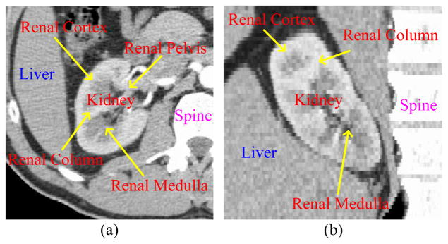
Image segmentation is a fundamental and challenging issue in the area of medical image analysis and computer-aided diagnosis. The kidney volume and renal cortex thickness are important clinical indications for renal function and are valuable for nephrologists. As shown in Fig. 1, the kidney consists of the renal cortex, renal medulla and renal pelvis. The renal cortex forms a continuous smooth outer zone with a number of projections (renal columns). Several kidney segmentation methods have been proposed in the literature [1–3]. They focused on mostly the whole kidney and seldom referred to the specific structures such as the renal column and renal cortex. Since the renal cortex thickness information plays an important role in renal function assessment, the segmentation of the renal cortex is desirable.

Fig. 1.

CT image of the kidney. (a) Coronal view. (b) Sagittal view.

Special characteristics of the kidney’s anatomical structure, such as (1) semi-closed structure around the renal pelvis, (2) weak boundaries between adjacent organs (e.g. liver, spine and muscles), and (3) the intensity proximity of the renal cortex and renal column (see Fig. 1), make renal cortex segmentation a challenging problem. Traditional methods such as region growing and threshold will most likely fail. Model-based methods incorporating anatomical constraints are necessary to separate the renal cortex and renal column. Furthermore, in order to overcome the weak boundaries, graph-based methods can be employed to search for a global optimal solution. In this paper, we propose an extended optimal surface search method [4] to segment the renal cortex by simultaneously extracting its outer and inner surfaces. The graph construction [5] was utilized to build a single graph for the entire image. However, it could not fully accommodate multiple surfaces, so we propose a new graph construction scheme that models multiple sub-graphs to address this problem.

2 Methods

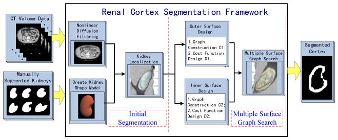
The framework of the proposed approach is illustrated in Fig. 2. The general strategy is to solve the renal cortex segmentation problem through multiple-surfaces extraction. The segmentation has two major stages. The first stage provides the approximate segmentation of the whole kidney, and the second stage simultaneously extracts the two surfaces.

Fig. 2.

The proposed renal cortex segmentation framework

2.1 Initial Segmentation

The initial segmentation is based on the statistical shape model method [6–7] and consists of the following three main steps: nonlinear diffusion filtering, kidney shape model creation and kidney initial localization.

1) Nonlinear diffusion filtering

As a preprocessing step, a nonlinear diffusion filter [8] is applied to smooth the image and reduce noise. The diffusion filter is defined by the following equation:

$$\{\begin{array}{l}\frac{\partial u(x,y,z,t)}{\partial t}=\mathit{div}[g({\mid \nabla u\mid }^2)\nabla u]\hfill \\ u(x,y,z,0)=u_0(x,y,z)\hfill \end{array}$$ (1)

t is a scale parameter, and the diffusivity function g(s) = 1−exp(−3.6150 (s/λ)10) if s> 0, and g (s) =1 otherwise. λ is the contrast parameter.

2) Kidney shape model creation

The kidney shape model is built from manually segmented kidneys in a training set. First, a triangulated surface mesh is reconstructed from the manually labeled images using marching cubes [9]. Then, a minimum description length (MDL) [10] approach is used to determine the point correspondence for all training shapes. Subsequently, all training shapes are aligned with affine transformations. Finally, the average kidney shape can be obtained with Φ̄=Σ_iΦ_i/n, where Φ_i is a training surface, and n is the number of the training set.

3) Kidney initial localization

After generating the average kidney shape, we can approximately locate this average shape using the software package Amira [11]. We use the built-in transformation editor to roughly register the average shape to the original volume.

2.2 Multiple-surface graph search

Based on the kidney initialization results, we employ an optimal surface search algorithm [4]. This algorithm can be considered as an optimization process aiming at finding the set of surfaces with the minimum cost. The three major components are graph construction, cost function design and optimal surface recovering.

1) Graph construction

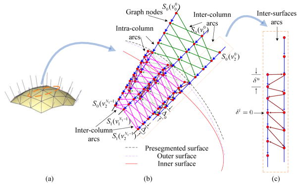
A key innovation of our method is its novel graph construction scheme, enabling construction of different sub-graphs according to different surface properties and inter-surface relationships. The graph construction process is illustrated in Fig. 3. Two sub-graphs (G₀,G₁) are constructed for outer and inner surfaces respectively in a narrowband around the surface meshes. For each vertex v_j on the mesh, a column of equidistant points is sampled along the normal direction of the vertex. The sampled points is denoted as $S_i(v_j^k)$, i = 0,1; j = 0, …, M −1; k = 0, …, N_i constituting the nodes for the sub-graphs, where i is the index of the two sub-graphs (G₀,G₁), j is the index of the vertex on the surface, and k is the index of the sampled points along the columns. We adopt different strategies to form the columns in sub-graphs G₀ and G₁, which are written in equ. 2:

$$\{\begin{array}{l}{S}_0(v_j^k)=v_j-(k-(N_0-1)/2)•{\mathrm{\Delta }}_0•\overrightarrow{n_j}(k=0,\dots ,N_0-1)\hfill \\ S_1(v_j^k)=v_j-k•{\mathrm{\Delta }}_1•\overrightarrow{n_j}(k=0,\dots ,N_1-1)\hfill \end{array}$$ (2)

where the normal direction $\overrightarrow{n_j}$ points outward, and (Δ₀,Δ₁) are the smoothness constraints for the two sub-graphs. The outer surface is searched both inward and outward, but the inner surface is searched only inward. This scheme is illustrated in Fig. 3(b)(c) so that G₀ spans both inside and outside of the pre-segmented surface and G₁ spans only inside the surface. This is based on the prior knowledge that the renal cortex inner surface should be inside of the initial exterior surface.

Fig. 3.

Graph construction. (a) Triangulated surface mesh with vertex normal. (b) Graph construction with three columns in the orange ellipse in (a). The whole graph is composed of two sub-graphs G₀ and G₁. The blue edges denote the intra-column arcs, while the green edges and red edges denote the inter-column arcs of the two sub-graph, and the brown edges between two columns projected from the same vertex denote the inter-surface arcs. (c) Detail of the inter-surfaces arcs.

There are three types of arcs in the graph shown in Fig. 3(b)(c):

$$\{\begin{array}{l}{E}^a=\left\{\langle S_i(v_j^k),S_i(v_j^{k-1})\rangle \mid i=0,1;j=0,\dots ,M-1;k=1,\dots ,N_i\right\}\hfill \\ E_i^r=\left\{\langle S_i(v_p^k),S_i(v_q^{max(0,k-{\mathrm{\Delta }}_i)})\rangle \mid \forall v_p,v_{q}is\mathit{adjacent};i=0,1;k=1,\dots ,N_i\right\}\hfill \\ E^s=\left\{\langle S_1(v_i^k),S_0(v_i^{k_l})\rangle ,\langle S_0(v_i^{k_u}),S_1(v_i^k)\rangle \mid {\delta }^l<\left(S_1(v_i^k)-S_0(v_i^{k_u}),S_1(v_i^k)-S_0(v_i^{k_l})\right)<{\delta }^u\right\}\hfill \end{array}$$ (3)

where (i, j, k) are the indices defined above. The intra-column arc E^a denoted by the blue edges connect two adjacent points on the same column; the inter-column arcs $E_0^r$ denoted by green edges connect two points on two adjacent columns of the outer surface sub-graph G₀, while the arcs $E_1^r$ are denoted by red edges in the inner surface sub-graph G₁; and the inter-surface arcs E^s denoted by the brown edges connect two points on different sub-graphs. In our graph construction, different smoothness constraints (Δ₀,Δ₁) are designed for the inter-column arcs in the two sub-graphs. Separation constraints (δ ^l,δ ^u) are exerted on the inter-surface arcs to separate the two surfaces.

2) Cost function design

All of the intra-column, inter-column and inter-surface arcs are viewed as n-links in the s–t graph [12] and assigned infinity values initially. Each node has a weight $W_i(v_j^k)$ in the weighted directed graph, where (i,j,k) are the indices defined in the previous section. The node weight $W_i(v_j^k)$ is defined below:

$$W_i(v_j^k)=\{\begin{array}{ll}{C}_i(v_j^k),••••••\hfill & k=0\hfill \\ C_i(v_j^k)-C_i(v_j^{k-1}),••\hfill & \mathit{otherwise}\hfill \end{array}$$ (4)

where the cost $C_i(v_j^k)$ is defined with cost functions reflecting some properties of the relevant surfaces. $C_0(v_j^k)$ and $C_1(v_j^k)$ represent the two cost functions for sub-graph G₀ and G₁:

$$\{\begin{array}{l}{C}_0(v_j^k)=-\mid \nabla I\left(v_j^k\right)\mid \hfill \\ C_1(v_j^k)=-F_{\mathit{sheet}}\left(I\left(v_j^k\right)\right)\hfill \end{array}$$ (5)

the 3-D “sheet filter” F_sheet [13] is defined as follows:

$$F_{\mathit{sheet}}\left(I\right)=\{\begin{array}{ll}\mid {\lambda }_3\mid ·w\left({\lambda }_2;{\lambda }_3\right)·w\left({\lambda }_1;{\lambda }_3\right)\hfill & {\lambda }_3<0\hfill \\ 0,\hfill & \mathit{otherwise}.\hfill \end{array}$$ (6)

λ₁, λ₂,λ₃(λ₁≥λ₂≥λ₃) are eigenvalues of Hessian matrix ∇²I, and w is written as

$$w\left({\lambda }_s;{\lambda }_t\right)=\{\begin{array}{ll}{\left(1+{\lambda }_s/\mid {\lambda }_t\mid \right)}^{\gamma }\hfill & {\lambda }_t\le {\lambda }_s\le 0\hfill \\ {\left(1-\alpha ·{\lambda }_s/\mid {\lambda }_t\mid \right)}^{\gamma }\hfill & \mid {\lambda }_t\mid /\alpha >{\lambda }_s>0\hfill \\ 0\hfill & \mathit{otherwise}\hfill \end{array}$$ (7)

where γ and α are parameters.

If $W_i(v_j^k)\ge 0$, nodes are connected to the sink terminal t by a directed edge with weight $W_i(v_j^k)$, otherwise nodes will be connected to the source terminal s by a directed edge of weight $-W_i(v_j^k)$. These arcs are t-links.

3) Optimal surface recovering

After the above two steps, a s–t graph G_st has been derived from the weighted directed graph G. Then we can apply the traditional graph cut algorithm [12] to recover the optimal surfaces. After that, the outer and inner surface meshes are scanned and converted to volumes with the same dimension and spacing as the original CT datasets. Finally, the segmentation of the renal cortex is obtained by subtracting the two volumes.

3 Experiments and Results

The proposed method was tested on 17 clinical CT datasets using Leave-one-Out cross validation. The CT images consist of 512×512×32 voxels. These data sets were manually segmented by labeling the kidney tissue to create kidney template images. Our method was implemented on a 32-bit desktop PC (2.33 GHz Core 2 and 2 GB RAM) based on the medical imaging toolkit [14] (MITK http://www.mitk.net/).

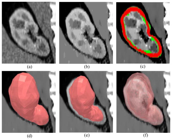
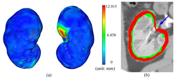
The parameters used in our algorithm are listed in Table 1. The sampling distance varies inversely with the density of local triangulated mesh. Results of the segmented renal cortex as well as the extracted outer and inner surface are shown in Fig. 4. Manual segmentation was used as reference and compared with the automatic segmentation result according to five metrics: true positive volume fraction (TPVF), false positive volume fraction (FPVF), signed relative volume difference (SVD), average symmetric surface distance (D_Avg), and average symmetric RMS surface distance (D_RMS). These metrics are summarized in Table 2. TPVF is relatively low compared to (1-FPVF), which is due mostly to the cortex segmentation error around the renal pelvis (blue arrow in Fig. 5(b)). Fig. 5(a) shows one example of the surface distance map between an automatic segmentation and a reference segmentation.

Table 1.

Parameter values

Stage	Parameter values
Initial segmentation	λ=10, step size 0.1, iter 30; n=17, model radius 0.3, samples number 41, landmarks 2562
Multiple surfaces graph search	Outer surface: N0=41, Δ0=1, sampling distance 0.2–4.0mm; Inner surface: N1=21, Δ1=1, sampling distance 0.1mm; M=2562, [δl,δu]=[3,8]sampling distance unit α = 0.5, γ = 0.25

Fig. 4.

Surface segmentation results. (a) Original image. (b) Enhanced image using nonlinear diffusion filtering. (c) Red region indicates the renal cortex segmentation result, while the reference segmentation is in green. (d) Outer surface mesh. (e) Inner surface mesh. (f) Combined segmented outer surface (translucent surface) and inner surface (wire frame).

Table 2.

Metrics results (Mean±SD)

TPVF(%)	FPVF(%)	SVD (%)	DAvg (mm)	DRMS (mm)
74.10±3.18	0.08±1.25	−3.46±3.33	0.69±0.20	1.36±0.29

Fig. 5.

(a) 3D surface distance map between the outer surface segmentation result and the kidney template image (ground truth). (b) Segmentation error around the renal pelvis (blue arrow). The cortex segmentation is in red, while the reference segmentation is in green.

4 Conclusions and Future Work

A novel approach has been presented to solve the renal cortex segmentation problem. We segment the renal outer and inner surfaces simultaneously by using the optimal multi-surface search method to generate the renal cortex. The experimental results demonstrate the effectiveness of the proposed method. Our key innovation is the novel graph construction scheme. Different surface sub-graphs are constructed according to the surface properties and inter-surface relationships. This graph construction scheme can be applied in other multiple-surfaces segmentation problems, such as the myocardium and cerebral cortex segmentation. In our future work, we will focus on improving the performance of inner surface segmentation. More investigations will be conducted about the separation constraints and cost functions, especially the relationship between the two cost functions.

References

- 1.Lin D, Lei C, Hung S. Computer-aided kidney segmentation on abdominal CT images. IEEE T Inf Technol Biomed. 2006;10(1):59–65. doi: 10.1109/titb.2005.855561. [DOI] [PubMed] [Google Scholar]
- 2.Cai W, et al. Dynamic-Threshold Level Set Method for Volumetry of Porcine Kidney in CT Images: In Vivo and Ex Vivo Assessment of the Accuracy of Volume Measurement. Acad Radiol. 2007;14(7):890–896. doi: 10.1016/j.acra.2007.03.005. [DOI] [PubMed] [Google Scholar]
- 3.Spiegel M, et al. Segmentation of kidneys using a new active shape model generation technique based on non-rigid image registration. Comput Med Imaging Graph. 2009;33(1):29–39. doi: 10.1016/j.compmedimag.2008.10.002. [DOI] [PubMed] [Google Scholar]
- 4.Li K, et al. Optimal surface segmentation in volumetric images - A graph-theoretic approach. IEEE Trans Pattern Anal Mach Intell. 2006;28(1):119–134. doi: 10.1109/TPAMI.2006.19. [DOI] [PMC free article] [PubMed] [Google Scholar]
- 5.Yin Y, et al. LOGISMOS-Layered Optimal Graph Image Segmentation of Multiple Objects and Surfaces: Cartilage Segmentation in the Knee Joint. IEEE Trans Med Imaging. 2010;29(12):2023–2037. doi: 10.1109/TMI.2010.2058861. [DOI] [PMC free article] [PubMed] [Google Scholar]
- 6.Heimann T, Meinzer H. Statistical shape models for 3D medical image segmentation: A review. Med Image Anal. 2009;13:543–563. doi: 10.1016/j.media.2009.05.004. [DOI] [PubMed] [Google Scholar]
- 7.Zhang X, et al. Automatic Liver Segmentation Using a Statistical Shape Model with Optimal Surface Detection. IEEE Trans Biomed Eng. 2010;57(10):2622–2626. doi: 10.1109/TBME.2010.2056369. [DOI] [PubMed] [Google Scholar]
- 8.Weickert J, Romeny B, Viergever M. Efficient and reliable schemes for nonlinear diffusion filtering. IEEE Trans Image Process. 1998;7(3):398–410. doi: 10.1109/83.661190. [DOI] [PubMed] [Google Scholar]
- 9.Lorensen WE, Cline HE. Marching cubes: A high resolution 3D surface construction algorithm. SIGGRAPH’ 87 Proceedings of the 14th annual conference on Computer graphics and interactive techniques; 1987. pp. 163–170. [Google Scholar]
- 10.Heimann T, et al. Implementing the automatic generation of 3d statistical shape models with itk. In MICCAI 2006 Open Source Workshop; Copenhagen, Denmark. 2006. [Google Scholar]
- 11.Stalling D, Westerhoff M, Hege H, Amira . The Visualization Handbook. Elsevier; Amsterdam: 2005. A highly interactive system for visual data analysis. [Google Scholar]
- 12.Boykov Y, Kolmogorov V. An experimental comparison of min-cut/max-flow algorithms for energy minimization in vision. IEEE Trans Pattern Anal Mach Intell. 2004;26(9):1124–1137. doi: 10.1109/TPAMI.2004.60. [DOI] [PubMed] [Google Scholar]
- 13.Sato Y, et al. Tissue classification based on 3D local intensity structures for volume rendering. IEEE Trans Vis Comput Graph. 2002;6(2):160–180. [Google Scholar]
- 14.Tian J, Xue J, Dai Y, et al. A novel software platform for medical image processing and analyzing. IEEE T Inf Technol Biomed. 2008;12:800–812. doi: 10.1109/TITB.2008.926395. [DOI] [PubMed] [Google Scholar]