On the utility of pooling biological samples in microarray experiments

Abstract

Over 15% of the data sets catalogued in the Gene Expression Omnibus Database involve RNA samples that have been pooled before hybridization. Pooling affects data quality and inference, but the exact effects are not yet known because pooling has not been systematically studied in the context of microarray experiments. Here we report on the results of an experiment designed to evaluate the utility of pooling and the impact on identifying differentially expressed genes. We find that inference for most genes is not adversely affected by pooling, and we recommend that pooling be done when fewer than three arrays are used in each condition. For larger designs, pooling does not significantly improve inferences if few subjects are pooled. The realized benefits in this case do not outweigh the price paid for loss of individual specific information. Pooling is beneficial when many subjects are pooled, provided that independent samples contribute to multiple pools.

Messenger RNA samples are often pooled in a microarray experiment out of necessity (1, 2) or in an effort to reduce the effects of biological variation (3–6). The idea behind the latter motivation is that differences due to subject-to-subject variation will be minimized, making substantive features easier to find (7–13). This is often desirable when primary interest is not on the individual (e.g., making a prognosis or diagnosis), but rather on characteristics of the population from which certain individuals are obtained (e.g., identifying biomarkers or expression patterns common across individuals). Because pooled designs allow for measurement of groups of individuals using relatively few arrays, they have the potential to decrease costs when arrays are expensive relative to samples.

Despite the potential advantages, pooled designs are often discouraged because of concerns regarding the inability to identify and appropriately transform or remove aberrant subjects and the inability to estimate within population variation. These concerns are uncontroversial when all subjects in a study are pooled and only technical replicates are obtained. However, there are pooling strategies that compromise between pooling everything and only considering individual biological samples on individual arrays. Theoretical advantages of such designs have been established (10, 11, 14). A brief review is given here.

A microarray experiment to estimate gene expression levels consists of extraction and labeling of RNA from n_s subjects, hybridization to n_a arrays, followed by scanning and image processing. Assuming that sufficient data preprocessing has been done to remove artifacts within and across a set of arrays, the gene expression measurements for a gene denoted by x₁, x₂,..., x_na are considered independent and identically distributed samples from a distribution with mean θ, the quantity of interest. The average of the measurements is used to estimate θ. Because the processed measurements are affected primarily by biological and technical variation, denoted and , respectively, the x_i are given by

Assuming that RNAs average out when pooled (biological averaging), , where r_s denotes the number of subjects contributing RNA to a pool and T_ik is the kth subject's contribution to the ith pool. Note that individual subjects contribute to one and only one pool, and in this way the pools contain biological replicates. Through biological averaging, the variability of ε_i is reduced to . The variance of the estimator for θ is then given by , where n_p is the total number of pools and r_a is the number of arrays probing each pool. The precision to estimate expression levels and the power to identify differentially expressed genes are inversely related to this variance, which is reduced by pooling because, for a pooled design, r_s > 1. The larger biological variability is relative to technical variability, the larger the overall variance reduction and benefit of the pooled design.

The utility of pooling in practice depends on the extent to which the assumed conditions hold for microarray data. Previous studies provide limited support for biological averaging (6) and variance reduction in pools (13), whereas one study recommends not pooling at all (15). In the latter study, a design with 16 arrays (eight individuals in two conditions) is compared to one with 2 arrays (pool of eight in each condition). Clearly, because the number of arrays is decreased without increasing the number of subjects, the two designs are not comparable; and, furthermore, questions regarding gene identification cannot be answered without biological replicates of both individuals and pools.

In short, key questions regarding the pooling debate remain unresolved:

1. To what extent is variability reduced by pooling?

2. Is biological variability larger than technical variability for most genes?

3. To what extent does biological averaging hold?

4. Are inferences regarding differential expression comparable for pooled and nonpooled designs?

We report here on the results of a large Affymetrix experiment with individuals and pools of varying sizes in two biological conditions designed to address these questions.

Methods

Supporting Information. For further details, see Supporting Text and Figs. 7–14, which are published as supporting information on the PNAS web site.

Data Collection. Thirty female inbred Wistar Furth rats were obtained from Harlan Sprague–Dawley at 5 weeks of age. The rats were group housed and provided Teklad diet (8604) and acidified water ad libitum. All rats were maintained with a light/dark cycle of 12 h. After a 2-week period of acclimation, rats were randomly assigned to a control or a retinoic X receptor treatment with an agonist LG100268, and were pair-fed every 24 h for 14 days. The experimental diets were prepared by adding LG100268, 100 mg per kg of diet meal (wt/wt), to the appropriate amount of ground rat meal diet and mixing for 15 min in an industrial size mixer in the chemical fume hood. All diets were double bagged and stored at –20°C for 1 week. Body weight was monitored by weighing at 2- or 3-day intervals. After consuming the diets for 14 days, rats were removed from the study for tissue collection.

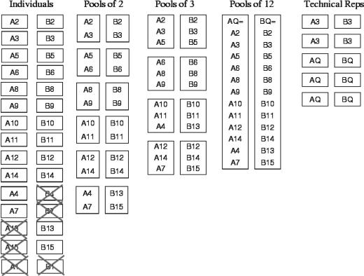
RNA samples were obtained from 15 rats in each condition. The estrus stage of each rat is provided in the data supplement. Four RNA samples were not sufficient for hybridization (see Fig. 1). Affymetrix RAE230A chips were used to measure gene expression for 15,923 genes for the remaining 26 animals. A1 and B1 were removed after preliminary analysis because they were farthest from other arrays in dendrograms similar to those shown in Figs. 8–10. The remaining 12 from each condition were chosen to construct 12 pools of pairs, 8 pools of triples, and 2 pools of 12 subjects. To obtain cRNA samples, total RNA was extracted from individual mammary glands; 5 μg of each RNA sample was reverse transcribed, synthesized to double-stranded cDNA, and then transcribed to biotin-labeled cRNA targets which were then fragmented. For the individuals, each chip was hybridized by using 10 μg of the fragmented cRNA targets; for the pools, equal amounts of fragmented targets were combined from the individuals to give a total of 10 μg. We note that the pooling was done after the labeling reactions, primarily to ensure enough starting material for individuals and multiple pools. When lack of sufficient tissue motivates pooling, samples would be combined before labeling and results could differ from those presented here. Within pool group, the processing of samples was randomized across treatments and Affymetrix scanners. To estimate technical variability, A3, B3, AQ, and BQ were analyzed using additional microarrays. Fig. 1 gives a schematic of the experiment. A single individual sample hybridized onto a single array is referred to as “1 on 1”; a pool of n subjects hybridized onto a single array is “n on 1”; M = n_p × n unique subjects hybridized onto n_p arrays (a pool of n onto each array) will be referred to as “M on n_p.” N technical replicates of a single array containing n subjects are denoted by “n on 1 × N.”

Fig. 1.

Schematic of the designed experiment. Each box represents one array; X's indicate samples that were not hybridized (A13, A15, B4, B7) or were hybridized but not used in construction of the pools (A1, B1). Here, A is control and B is treatment.

Preprocessing and Normalization. Robust multiarray analysis (RMA) was used to preprocess and normalize the raw Affymetrix GeneChip data (16). Individuals, pools, and technical replicates were processed together. RMA fits a linear model to the log probe intensities for each probe set. The linear model includes a sample effect, a probe effect, and an error term. Fig. 7 shows standard error estimates of the sample effects for each array. Because RMA has been shown to give very low false-positive rates without filtering, and potentially inflated false-negative rates after filtering, all 15,923 genes were used in the analysis. RMA has been demonstrated to provide improved precision over the default algorithms provided by Affymetrix, which generates mas5.0 signals (17). We observe similar findings for this data set (Figs. 8–10).

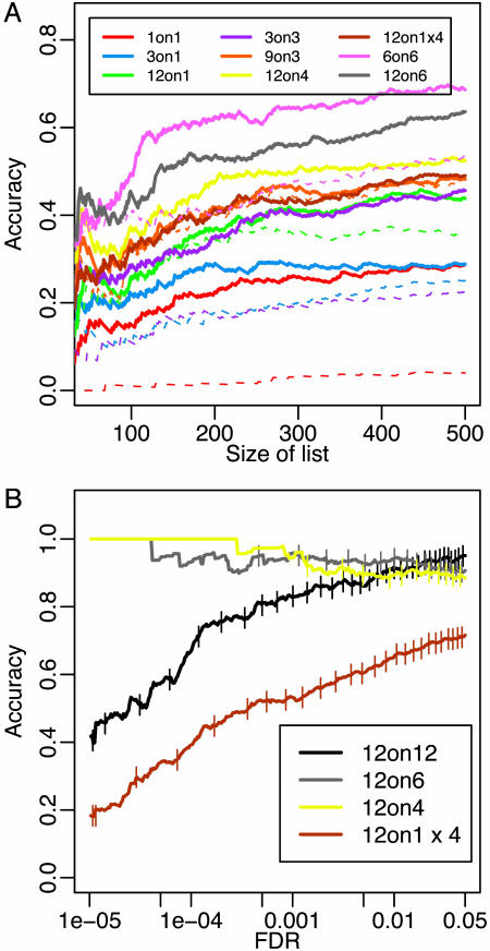
Comparison of Designs. For each design, moderated t statistics (18) between control and treatment samples were obtained for every gene if more than three arrays were available (see Supporting Text). With fewer than three arrays, a fold change was calculated. For the rank plot (see Fig. 6A), the statistics were ranked from largest to smallest. The top N genes made up a list of size N. For the false discovery rate (FDR) plot (see Fig. 6B), the FDR of a list was estimated by using the q value approach (19). Each color in each plot represents one potential design and reports the percentage of differentially expressed (DE) calls in common between that design and a reference for lists of fixed size or fixed FDR (note that lists with fixed FDR may vary in size). The reference list was generated by using Student's t statistics calculated on the full set of 12 individuals in each condition. The percentage in common is referred to as accuracy. Each vertical tick on the FDR plot marks 100 genes identified at the specified level of FDR. For some designs, a number of subsets could be chosen to generate a list. For example, with a 3 on 3 design, subsets were possible. We considered all subsets (or 100 subsets at random if >100 were available). The solid line gives an average performer across the subsets; the dashed line gives the worst case performer. Plots were also generated by using reference lists obtained from a Wilcoxon statistic and a statistic measuring the posterior odds of differential expression (20). Results remained unchanged.

Fig. 6.

Design accuracy. (A) Lists of fixed size. Solid lines give the average performer across 100 subsets; dashed lines give the worst case performer. (B) Lists with fixed FDR. Each vertical tick on the FDR plot marks 100 genes identified at the specified level of FDR (see Comparison of Designs for more details on the construction of each figure). Virtually identical results were obtained if CEL files were processed by using RMA within pool group (see Fig. 12).

Results

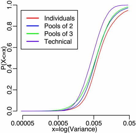
Pooling Reduces Overall Variability. Gene-specific sample variances were calculated across conditions for individual samples, pools of 2 and 3, and technical replicates. Fig. 2 shows nearly perfect stochastic ordering with decreasing variability from individuals to technical replicates. However, this trend does not hold for each gene. Variability across technical replicates was larger than variability across individuals for 31% of the genes. The negligible biological variability estimated here may be due to truly small biological variability or to poorly designed probe sets that allow for little hybridization or sufficient cross-hybridization. Whatever the reason, for genes with relatively small biological variability, there are negligible gains by pooling.

Fig. 2.

Gene-specific sample variances: cumulative distribution functions of gene specific sample variances are calculated by combining estimates across biological conditions. Density estimates are shown in Fig. 11.

Pooling Results in Biological Averaging for Most Genes. To investigate whether RNA samples average out when pooled (biological averaging), mathematical averages (referred to here as averages) across individuals were compared to the corresponding pools. Some distortion is expected as the original RNA abundance undergoes a series of possibly nonlinear transformations during the measurement process. In the absence of pooling, individual samples are transformed separately, whereas when pooling is done, the transformation applies to the pool rather than to each individual sample. Any averaging that takes place on the scale of raw RNA abundance is transformed during data generation and processing, and as a result measurements from a pool may not correspond to an average of individual samples that comprise the pool.

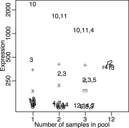
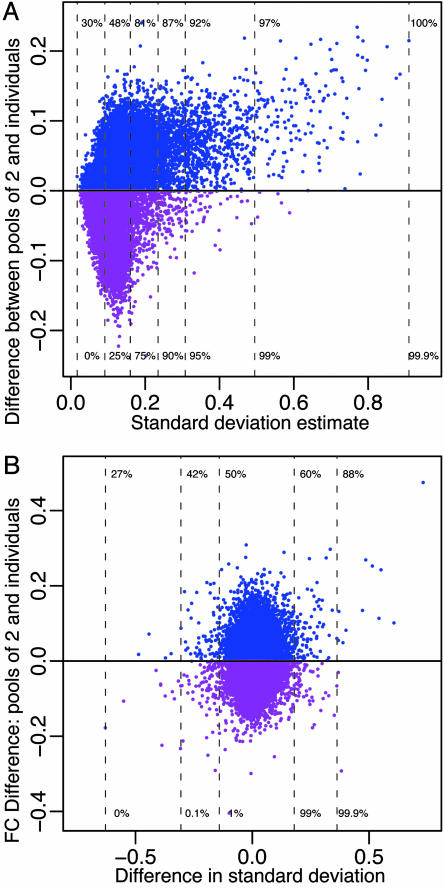
Fig. 3 gives an example. Shown is one gene where the averages on the raw intensity scale are quite similar across the individuals and pools. After a log transformation, as often recommended for microarray data (20–25), the averages in the individuals are smaller than those in the pools. This is a biological realization of the well known Jensen's inequality (26), which states that the average of log transformed values will always be less than or equal to the log of the average of the untransformed values. The fact that we observe this difference here is evidence of biological averaging (pools look like an average of untransformed individual values). The difference between the average of the log individuals and the log of the pools is exacerbated by outliers (e.g., arrays 3 and 10 in Fig. 3). Part of the reason for this is that for the case of individuals, outliers are first attenuated by a log transform and then averaged. For the pools, the attenuation has less of an effect because the outlier has already been averaged with other samples. Fig. 4A shows that this artifact affects ≈25% of the genes.

Fig. 3.

Distorted gene. Expression values are shown for individuals, pools, and technical replicates. The + (x) indicates the mathematical average of the raw (log) data; the m indicates the median of the values. The numbers refer to arrays (control condition). Of importance here are arrays 3 and 10, where expression values for this gene differ from the majority. The effects of arrays 3 and 10 are attenuated by the values they are pooled with (11 and 2, respectively, for the pools of two).

Fig. 4.

Effects of distortion within and between conditions. (A) The mean difference between the pools of two and the corresponding averages across individuals (control condition) as a function of standard deviation (SD) estimated within the control condition (all genes are shown). The units are log base-2 expression. The percentiles of SD are shown (bottom) along with the percentage of genes (top) having values in the pools of two that are larger than the corresponding average across individuals. Genes with values in the pools that are higher (lower) than the corresponding averages are shown in blue (purple). For the 25% of the genes with largest SD, >80% have values larger in the pools of two. Similar results were found by using estimates of either technical or biological SD. The treatment condition and pools of three give similar results. (B) The difference between the log fold change (FC) values (control/treatment) calculated from the pools of two and the individuals for the genes shown in A plotted as a function of the difference in SD calculated across conditions. B is unitless because we are considering the difference in log fold change. Distortion affects both control and treatment and largely cancels out when FCs are considered resulting in similar FC values in the individuals and pools.

Another factor potentially affecting agreement between pools and their averages is that the actual amount of individual RNA contributing to each pool may vary across individuals, despite careful quality control measures. The effects of this on pooling have been considered (27). Despite distortions, we find that pools are more similar to averages of the contributing samples than they are to other pools (Fig. 13). Furthermore, the dendrogram in Fig. 9 shows that pools of two cluster closely with their averages. The same holds for pools of three. These plots suggest that biological averaging occurs for most, but not all genes. Furthermore, for the genes where biological averaging does not occur, similar amounts of distortion are often observed in both control and treatment conditions and, as a result, the identification of DE genes is not grossly affected (Fig. 4B).

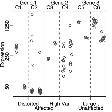
Identifying Differentially Expressed Genes. Designs without biological replicates. Without biological replication, outliers cannot be found and appropriate variance components cannot be estimated. Fig. 5 gives an example of how this can adversely affect DE inferences. Each affected gene appears to be DE when only technical replicates are considered. It is clear when biological replicates are available that the first DE call is caused by outliers and the second DE call is caused by an underestimation of the gene-specific variance. The last gene shown is not affected by an outlier. Correct inferences regarding DE would be made in this case using only technical replicates. Fig. 6A shows that this latter case is most representative of the full data set as similar lists of DE genes are identified when using true biological replicates (e.g., 12 on 4 ≈ 12 on 1 × 4; see Methods for terminology). In fact, the same level of accuracy is only slightly reduced when single arrays with pools of 12 (12 on 1) are considered. This is not the case when pooling is not done. An analysis using individuals on single arrays (1 on 1) reduces accuracy by ≈50%. Pooled designs with biological replication. When the RNA from an individual contributes to one and only one pool, and many pools are constructed, the pools can be used to properly assess biological variation. Pooling extra subjects onto a fixed number of arrays decreases variability across experiments and provides a representative list of genes with accuracy similar to the representative lists obtained without pooling (Fig. 6A). For example, the representative lists from an analysis of 3 on 3, 6 on 3, or 9 on 3 have similar accuracy. However, the variability across the 9 on 3 experiments is reduced, resulting in a list for a particular experiment that has properties near those of the representative list. Similar results are found for other comparisons. Reducing the number of arrays in an experiment without increasing the number of subjects decreases accuracy (Fig. 6A).

Fig. 5.

DE inferences without biological replication. Expression values from three genes are shown. Technical replicates for genes 1 and 2 are shown in columns C1 and C3. By considering these technical replicates only, the first two genes might be considered DE by some measures (because the averages in each group are quite different); when biological replicates are considered for these two genes (columns C2 and C4), it is obvious that the difference in means is caused by three outliers (first gene) and underestimation of the biological variance (second gene). DE calls for gene 3 would be the same, whether considering biological or technical replicates; +, x, and m are defined in Fig. 3.

False discovery rate (FDR) control. Designs in Fig. 6A are compared based on agreement among the top ranking genes for lists with fixed size. For these comparisons, no consideration of the FDR associated with each list is made. Results regarding accuracy are very similar when comparisons are instead made among lists with fixed FDR. There is one major difference: when biological replicates are not available and technical replicates are used, estimates of the variance required for FDR specification are incorrect, resulting in many DE calls with very low accuracy (Fig. 6B). Fig. 6B also provides insight into how the number of genes identified as DE by an FDR-based criterion varies among the designs. As the number of arrays decreases for a fixed number of subjects, fewer genes are identified as DE. This reduction is expected, because to have comparable results while decreasing the number of arrays, one must increase the number of subjects appropriately to maintain a so-called “equivalent” design.

Equivalent designs. Formulas exist specifying the number of subjects and arrays required in a pooled design so that gene specific (10) or average (11) estimation efficiency is maintained comparable to a design where pooling is not done and additional arrays are used (see Supporting Text). Similar formulas hold when equivalent power is considered. Given the biological and technical variability in this study, the following designs are equivalent: 100 on 100 vs. 160 on 80; 25 on 25 vs. 42 on 21; 7 on 7 vs. 12 on 6. Fig. 14 shows that there is little difference between the genes identified from the last designs. However, although the designs are equivalent on average, gene-specific DE calls are affected by varying biological and technical variability; and, as a result, pooling while reducing the number of arrays will be useful for identifying some genes, at the expense of not identifying others.

Discussion

Experimental designs using pooled RNA samples are often done out of necessity or in an effort to reduce the effects of biological variation, making substantive differences easier to find. Pooled designs are attractive because they have the potential to decrease cost due to the fact that a large number of individual samples can be evaluated using relatively few arrays. Here, we have considered fundamental properties of various pooling designs to evaluate their performance and to determine whether the basic conditions required for pooling to be useful hold.

The most basic condition is the assumption of biological averaging. Many investigators conjecture that RNA abundance levels average out when pooled. This may be true; however, because of nonlinearities introduced in the generation and processing of microarray data, an average on the scale of raw RNA abundance will not necessarily correspond to the average of the same highly processed RNA measurements. The log transformation was found to affect ≈25% of the genes (some distortion also appears on the raw intensity scale; this is not considered here because data are almost always transformed before analysis; refs. 20–25). There may also be implicit transformations that could affect the measurements; despite these, we found that most expression measurements from RNA pools are similar to averages of individuals that comprise the pool. For the majority of genes where there was a large difference, the difference was similar across biological conditions, resulting in comparable DE inferences from individuals and pools. Because of this, pooled designs were never found to perform significantly worse than nonpooled designs.

For very small designs in which only one or two arrays are available in each biological condition, pooling dramatically improves accuracy. Although valid, the results in such small designs are limited as gene specific variance components cannot be well estimated and outliers cannot be identified. Designs involving technical replicates only are similarly limited; and when used with statistical methods that require estimates of both biological and technical variability (e.g., FDR-based methods), they can be very misleading. When the goal of the experiment is to identify DE genes, investigators should favor biological, not technical, replicates.

For larger designs where biological replicates are used, pooling is not always advantageous. Accuracy was similar across designs in both the rank and FDR based analyses when the number of arrays was fixed and the number of subjects varied. There is a slight decrease in the variability among the lists of DE genes identified as the number of subjects pooled increased; but the modest reduction resulting from pooling two to three subjects per array is generally not worth the price paid for loss of individual specific information. A greater advantage can be gained by pooling a larger number of subjects. For a fixed number of subjects, reducing the number of arrays results in decreasing accuracy and fewer genes with small FDR. This result is expected, because to maintain equivalent properties, the number of subjects pooled must be increased appropriately.

An optimal method for specifying equivalent designs will depend on a number of factors (see Supporting Text). To the extent that simplified models of equivalence hold (10, 11), we found the following designs to be equivalent for this data set: 100 on 100 vs. 160 on 80; 25 on 25 vs. 42 on 21; 7 on 7 vs. 12 on 6; evidence for equivalence was given in the last case. The financial benefit of pooling for this particular case is minimal at best. However, the results demonstrate the potential of equivalent design specification. For larger designs, the realized benefit of decreasing the number of arrays can be substantial. Furthermore, in studies of humans, biological variability is generally larger than technical variability (28), the condition that yields a greater reduction in the number of arrays required. Experiments to estimate gene-specific variance components and validate the conditions considered here should prove quite useful for extrapolating these results to other systems and addressing other questions of microarray experimental design.

References

- 1.Jin, W., Riley, R. M., Wolfinger, R. D., White, K. P., Passador-Gurgel, G. & Gibson, G. (2001) Nat. Genet. 29, 389–395. [DOI] [PubMed] [Google Scholar]
- 2.Saban, M. R., Hellmich, H., Nguyen, N., Winston, J., Hammond, T. G. & Saban, R. (2001) Physiol. Genomics 5, 147–160. [DOI] [PubMed] [Google Scholar]
- 3.Chabas, D., Baranzini, S. E., Mitchell, D., Bernard, C. C., Rittling, S. R., Denhardt, D. T., Sobel, R. A., Lock, C., Karpuj, M., Pedotti, R., et al. (2001) Science 294, 1731–1735. [DOI] [PubMed] [Google Scholar]
- 4.Waring, J. F., Jolly, R. A., Ciurlionis, R., Lum, P. Y., Praestgaard, J. T., Morfitt, D. C., Buratto, B., Roberts, C., Schadt, E. & Ulrich, R. G. (2001) Toxicol. Appl. Pharmacol. 175, 28–42. [DOI] [PubMed] [Google Scholar]
- 5.Enard, W., Khaitovich, P., Klose, J., Zollner, S., Heissig, F., Giavalisco, P., Nieselt-Struwe, K., Muchmore, E., Varki, A., Ravid, R., et al. (2002) Science, 296, 340–343. [DOI] [PubMed] [Google Scholar]
- 6.Agrawal, D., Chen, T., Irby, R., Quackenbush, J., Chambers, A. F., Szabo, M., Cantor, A., Coppola, D. & Yeatman, T. J. (2002) J. Natl. Cancer Inst. 94, 513–521. [DOI] [PubMed] [Google Scholar]
- 7.Churchill, G. A. & Oliver, B. (2001) Nat. Genet. 29, 355–356. [DOI] [PubMed] [Google Scholar]
- 8.Simon, R. M. & Dobbin, K. (2003) BioTechniques 34, 516–521. [Google Scholar]
- 9.Churchill, G. A. (2002) Nat. Genet. Suppl. 32, 490–495. [DOI] [PubMed] [Google Scholar]
- 10.Kendziorski, C. M., Zhang, Y., Lan, H. & Attie, A. (2003) Biostatistics 4, 465–477. [DOI] [PubMed] [Google Scholar]
- 11.Kendziorski, C. (in press) in DNA Microarrays and Statistical Genomics Techniques: Design, Analysis, and Interpretation of Experiments. eds. Allison, D. B., Page, G., Beasley, T. M. & Edwards, J. W. (Marcel Dekker, New York).
- 12.Allison, D. B. (2002) Proceedings of the American Statistical Association, Biopharmaceutical Section (Am. Stat. Assoc. Press, Alexandria, VA), pp. 37–44.
- 13.Han, E. S., Wu, Y., McCarter, R., Nelson, J. F., Richardson, A. & Hilsenbeck, S. G. (2004) J. Gentrol. 59A, 306–315. [DOI] [PubMed] [Google Scholar]
- 14.Peng, X., Wood, C. L., Blalock, E. M., Chen, K. C., Landfield, P. W. & Stromberg, A. J. (2003) BMC Bioinformatics 4, 26. [DOI] [PMC free article] [PubMed] [Google Scholar]
- 15.Affymetrix (2004) Sample Pooling for Microarray Analysis (Affymetrix, San Diego), technical note.
- 16.Irizarry, R. A., Hobbs, B., Collin, F., Beazer-Barclay, Y. D., Antonellis, K. J., Scherf, U. & Speed, T. P. (2003) Biostatistics 4, 249–264. [DOI] [PubMed] [Google Scholar]
- 17.Irizarry, R. A., Bolstad B. M., Collin, F., Cope, L. M., Hobbs, B. & Speed, T. P. (2003) Nucleic Acids Res. 31, e15. [DOI] [PMC free article] [PubMed] [Google Scholar]
- 18.Smyth, G. K. (2004) Stat. Appl. Genet. Mol. Biol. 3, 3. [DOI] [PubMed] [Google Scholar]
- 19.Storey, J. D. & Tibshirani, R. (2003) Proc. Natl. Acad. Sci. USA 100, 9440–9445. [DOI] [PMC free article] [PubMed] [Google Scholar]
- 20.Kendziorski, C. M., Newton, M. A. Lan, H. & Gould, M. N. (2003) Stat. Med. 22, 3899–3914. [DOI] [PubMed] [Google Scholar]
- 21.Kerr, M. K., Martin, M. & Churchill, G. A. (2000) J. Comput. Biol. 7, 819–837. [DOI] [PubMed] [Google Scholar]
- 22.Lonnstedt, I. & Speed, T. P. (2002) Statistica Sinica 12, 31–46. [Google Scholar]
- 23.Quackenbush, J. (2001) Nat. Rev. Genet. 2, 418–427. [DOI] [PubMed] [Google Scholar]
- 24.Wolfinger, R. D., Gibson, G., Wolfinger, E. D., Bennett, L., Hamadeh, H., Bushel, P., Afshari, C. & Paules, R. (2001) J. Comput. Biol. 8, 625–637. [DOI] [PubMed] [Google Scholar]
- 25.Yang, Y. H., Dudoit, S., Luu, P., Lin, D. M., Peng, V., Ngai, J. & Speed, T. P. (2002) Nucleic Acids Res. 30, e15. [DOI] [PMC free article] [PubMed] [Google Scholar]
- 26.Jensen, J. (1906) Acta Mathematica 30, 175–193. [Google Scholar]
- 27.Ji, Y.. (2003) Ph.D. thesis (University of Wisconsin, Madison).
- 28.Cheung, V. Conlin, L. K., Weber, T. M., Arcaro, M., Jen, K. Y., Morley, M. & Spielman, R. S. (2003) Nat. Genet. 33, 422–425. [DOI] [PubMed] [Google Scholar]
Associated Data
This section collects any data citations, data availability statements, or supplementary materials included in this article.