Variable Threshold Method for Determining the Boundaries of Imaged Subvisible Particles

Abstract

An accurate assessment of particle characteristics and concentrations in pharmaceutical products by flow imaging requires accurate particle sizing and morphological analysis. Analysis of images begins with the definition of particle boundaries. Commonly a single threshold defines the level for a pixel in the image to be included in the detection of particles, but depending on the threshold level, this results in either missing translucent particles or oversizing of less transparent particles due to the halos and gradients in intensity near the particle boundaries. We have developed an imaging analysis algorithm that sets the threshold for a particle based on the maximum gray value of the particle. We show that this results in tighter boundaries for particles with high contrast, while conserving the number of highly translucent particles detected. The method is implemented as a plugin for FIJI, an open-source image analysis software. The method is tested for calibration beads in water and glycerol/water solutions, a suspension of microfabricated rods, and stir-stressed aggregates made from IgG. The result is that appropriate thresholds are automatically set for solutions with a range of particle properties, and that improved boundaries will allow for more accurate sizing results and potentially improved particle classification studies.

INTRODUCTION

The flow imaging method of particle size analysis has proven increasingly popular for the analysis of biotherapeutics¹. Compared to other methods, flow imaging is less sensitive to particle refractive index than light obscuration^2,3,4, and image parameters reported by flow imaging enable classification of particles by morphology and brightness. Commercial flow imaging instruments have an optical resolution of approximately 1 μm to 4 μm, yet these instruments are routinely used to size particles down to 2 μm effective diameter. Properly interpreting the particle boundary is key to obtaining accurate particle size and morphology, especially for particles below ≈ 5 μm effective diameter.

The flow imaging method of particle size analysis relies on the definition of the particle boundary by image processing software. In commercial instruments, it is common to obtain a background image during the acquisition process. A threshold is set to distinguish the brightness of a pixel that is part of a particle in a collected image, from that same pixel brightness in the background image. Depending on the properties of the particle and its position relative to the focal plane, the presence of the particle may result in some pixels brighter than the background and some darker. Some instruments allow for both bright and dark thresholds to allow for both possibilities^3,5.

It has been recognized that, depending on composition, some particles have a large index of refraction difference from the fluid they are in (for example polystyrene calibration beads) and appear with high contrast, while other particles are nearly transparent and appear only slightly different in brightness from the background^2,6. Furthermore, there is commonly a halo around the edges of the particle due to out-of-focus and diffraction effects⁷. These halos can vary with particle size and particle contrast. Due to these effects, there can be a dependence on the measured size of a particle on the threshold selected for the measurement, and this dependence can introduce errors and ambiguities in the measured particle size³. These effects become even more important for elongated particles, where a perimeter-based calculation of particle-dimension can improve the sizing results⁸. Some users will set a different threshold depending on the anticipated properties of particles they expect to measure; however, it is not unusual for a protein drug sample to contain a variety of particle types over a broad size range. For such a sample, the use of a single threshold can lead to measurement errors.

For some particle imaging applications, algorithms have been developed to correct for some of the effects described above. Xu et al. developed an algorithm for measuring bubbles in a fluid that sorts for bubbles in focus⁹. Dahl et al. modeled the appearance of a particle at different locations with respect to the focal plane¹⁰. This model was tested using 25 μm beads, which had a refractive index of 1.6. Pedersen et al. applied the variance filter in ImageJ to the image for the purpose of detecting translucent particles and reducing fragmentation effects¹¹. As a result of this process, particles with large gradients will have a band that extends further away from the particle than for nearly translucent particles. The fixed threshold used to convert to a binary image will pick up the outer boundary of the threshold gradient, which is larger for darker particles; therefore particles with larger gradients will be oversized.

Because samples may contain a variety of particles, and because it would be desirable to run calibration samples under the same conditions as test samples, it would be desirable to have an image processing system that does not require the user to anticipate the particle properties to set run conditions. It would be preferable to have an algorithm adjust the threshold for boundary determination based on the properties of each particle identified. Example properties would be the maximum, average, or minimum gray value, or the maximum gradient value. These values depend on the background removal method employed and how pixels brighter and darker than background are treated. We have developed a variable threshold algorithm for processing particle images that gives improved boundaries that translate to more accurate sizing as well as improved shape parameter values.

MATERIALS AND METHODS

Polystyrene beads of reported 2.0 μm, 5.0 μm and 10.1 μm diameter were obtained in aqueous suspensions from Beckman Coulter, Inc. (Brea, CA)¹². Beads were diluted in ultrafiltered, deionized water (Barnstead Nanopure system, Dubuque, IA). Since polystyrene beads have refractive index n of n=1.59, which is far from water (n=1.33), while protein aggregates have an index between 1.33 and ≈1.4, it was useful also to do a test using silica beads with n≈1.4 {Hu, 2015 #175}. Monodisperse silica beads with reported diameters of 4.08 μm and 6.10 μm diameter with refractive indices of n=1.44 and n=1.42, respectively, were obtained in dry form from Cospherics (Santa Barbara, CA), and Bangs Laboratories (Fishers, IN), respectively¹². Anhydrous glycerol was purchased from JT Baker (Center Valley, PA) and sodium azide solution was obtained from Ricca Chemical (Arlington, TX). A stock bead solution was prepared by adding the dry beads to filtered water containing 0.02 % mass concentration sodium azide, shaking vigorously for 40 s, sonicating for 20 s, and inverting 10 times gently prior to further dilution. To prepare the 1.43 refractive index solution, pure glycerol was diluted into deionized water to prepare a 86 % mass concentration glycerol-water solution and filtered through a 0.45 μm polyvinylidene difluoride (PVDF) filter. The silica bead stocks were diluted 77 fold for the 6.10 μm beads, and 111 fold for the 4.08 μm beads, into deionized ultrafiltered water or into glycerol water solution to obtain solutions with n=1.33 and n=1.43 at the sodium D line, respectively, which was verified with an Abbe Refractometer (Vista C10). The n=1.43 solution was used to match the index of refraction of the silica beads and simulate the small index refraction difference between buffer and protein aggregates.

Rods were fabricated using photolithography as described previously⁸. Briefly, an epoxy-based negative photoresist SU-8 (MicroChem Corporation, Newton, MA) was deposited by spinning it at 1800 revolutions per minute over a thin release layer onto a silicon wafer. The SU-8 was exposed to ultraviolet light through a mask and baked to selectively polymerize the particles. Unexposed SU-8 was removed in a solution of developer. The release layer was then dissolved resulting in a suspension of rods. Allowing the rods to settle to the bottom, the solvent was exchanged for water by pipetting. Rod dimensions by electron microscopy were (41.4 ± 0.2) μm long × (2.80 ± 0.07) μm × wide (2.57 ± 0.02) μm thick (all uncertainties expressed as standard uncertainties). Nominal concentrations were 1000 particles per milliliter.

To prepare IgG aggregates by agitation, a polyclonal human IgG was obtained from Sigma Aldrich (Catalog number I2511, St. Louis, MO). Prior to use, it was diluted into a 0.30 mg/mL sodium phosphate buffer, passed through a 0.22 μm filter, and split into 11 mL aliquots in three precleaned perfluoroalkoxy (PFA) vials. To generate the aggregates, the IgG protein solution vials were placed on a rotator that inverted the vials once every 7.5 s for 16 h to 17 h. This produced a particle concentration of 5×10⁴ mL⁻¹ greater than one micrometer as measured by Instrument A described below.

Two instruments were used for flow imaging. Most of the measurements were made using Instrument A which was a FlowCam (Fluid Imaging Technologies Inc., Yarmouth, Maine) with a 100 μm flow cell and a 10× microscope objective. The camera operated in auto image mode at a flow rate of 0.20 mL/min, capture rate of 9 and 15 frames per second (fps), and efficiency of 10 % and 17 % for protein aggregate and bead samples respectively. Image data files were stored as TIF files. To show the algorithm described in this paper is of general use by different flow imaging methods, a second instrument was used for the measurements of silica beads. Instrument B was a Micro-Flow Imaging (MFI) DPA-4200 (ProteinSimple, San Jose, CA; settings: 100 μm thick flow cell, at “SP3” optical configuration). For each run, 0.7 mL of sample was loaded, of which 0.2 mL was the purge volume. The samples were run at 0.17 mL/min and the optimize illumination protocol was performed with the sample. Run parameters used by the two instruments are summarized in Table 1. Silica beads in the n = 1.33 refractive index solution were sonicated for 20 s, inverted 10 times, and pipetted 10 times prior to analysis. Since the n = 1.43 refractive index solution was more viscous and prone to air bubble formation, the particles were mixed by gentle tilting and rotating of the sample vial. For analyses of these samples, the instrument’s flow cell was allowed to run dry then 0.4 mL sample was loaded at a rate of 0.3 mL/min until the flow cell was filled with the solution and the refractive index with homogeneous throughout the flow cell. Following this, 0.7 mL more of the sample was loaded and analyzed. Particle images, morphology information, size distribution, and concentrations were obtained using the MFI’s MVAS 1.3 software. Image data files were stored as JPG files. Only the image files were used from both instruments. In addition to these instruments, a Leica DMRX microscope was used for imaging protein aggregates at different focal points. Vertical position of a 20×/0.4 NA microscope objective was computer-controlled using a Piezosystem Jena NV40/1CL E objective scanner through Micro-Manager software¹³. These images were captured using a Lumenera Infinity 2–2M camera.

Table 1.

Summary of flow imaging parameters for two instruments.

Instrument	Magnification	Flow Cell thickness (μm)	Acquisition Rate (fps)	Efficiency (%)	Flow Rate (mL/min)	Sample Volume Processed (mL)
A	10×	100	9 and 15	10 and 17	0.200	0.5
B	Not available	100	7	85	0. 17	0.5

The steps in the algorithm for processing images is indicated in Figure 1, a schematic flow diagram of the process steps, and Figure 2, an example using an acquired image. Raw image files from the flow imaging instruments or microscope were transferred to a computer with the open source software known as “FIJI”¹⁴ which is a combination of ImageJ¹⁵ and a set of additional plug-ins. This algorithm is implemented as a plugin for FIJI written in Java and available through GitHub¹⁶. Prior to operating the plugin, the images are imported as a image sequence into FIJI which results in an image “stack”. If necessary the images are converted to 256 bit grayscale images and the stack is saved to the computer. With the image open, the plugin “Variable_Threshold” is selected by the user. Figure 2a shows an example portion of a single image from a stack.

Figure 1.

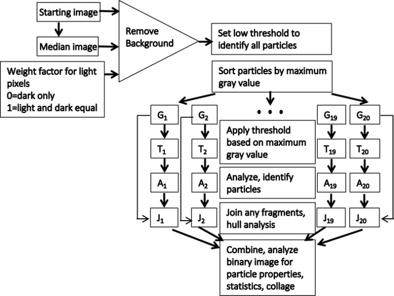
Flow chart of process steps used in variable threshold algorithm.

Figure 2.

Example of variable threshold algorithm. (a) Example image of protein aggregates, part of an image stack, captured by flow imaging equipment. (b) Image from (a) after an absolute value background subtraction and a threshold process—all pixels from the background subtraction with gray values greater than 8 are assigned the value 1 in the resulting binary image, all other pixels are assigned the value 0. (c) The binary image in (b) is analyzed for particles. The analysis returns regions of interest (ROI), referenced to the background-subtracted image. These ROI’s are sorted according to maximum gray value (from the referenced image), to create a set of binary images consisting of particles of binned maximum gray values. (d) The binary images from (c) are used as masks for the binary subtracted image to create a set of grayscale images. The grayscale images are then subjected to a thresholding process with a threshold that is 0.5 times the value of maximum gray value corresponding to the sorted value used to create the mask in (c). The set of images in (d) are the resulting binary images from this thresholding process.

For clarity, (to increase the size of the particles) images (b)-(e) were enhanced with a “dilate” binary image process.

The Variable_Threshold plugin begins by obtaining a background image by finding the median image intensity for each pixel of the image stack. The background image is then subtracted from the image stack. This subtraction can be done as an absolute value subtraction (equal weight to “light” (brighter than background) and “dark” (darker than background) pixels), which is typical for Instrument A analysis. For Instrument B, and optionally for Instrument A, thresholding is based only on pixels darker than the background, and the image stack is subtracted from the background image. The plugin also allows for user selected weighting of light and dark pixels (also available on Instrument A software).

Once the background is removed, a threshold is applied to the image stack. This threshold is selected by the user to have a low enough value to pick up the faintest particles, but not noise. A typical value is (4 to 10)% of the average gray value of the image. We used the value 8 for the initial threshold. For flow instrument A, a variety of threshold values have been used between 8 and 20.^17,18,19 The result of the threshold process is a binary image as shown in Figure 2b. This binary image is subjected to a dilate/fill holes/erode sequence which removes holes and smooths the boundary of particle regions. The FIJI “Analyze Particles” routine is called with reference to the background-subtracted image stack. The result is a large number of “regions of interest” or ROI’s appearing in the FIJI RoiManager. Each ROI refers to an identified particle in the binary image, with an associated set of properties from the corresponding background-subtracted image.

Among these properties, the plugin makes use of the “maximum gray value” of the ROI. An array of the maximum gray value represents all the particles in the background-subtracted image stack. The ROIs are sorted into bins according to values of the associated maximum gray value, and the corresponding regions from the binary image stack (i.e., Fig 2b) images are pasted in a separate temporary binary image stack for each gray-value bin. The result is a set of typically 20 temporary binary image stacks; each stack is like the original binary image stack, but it only has the images of particles for a particular gray-value bin. Figure 2c shows an example with 5 (instead of 20 for simplicity) temporary binary images. One can identify that the particles from Figure 2b have been sorted into the 5 images in Figure 2c, with the brightest particles in the rightmost image. The resulting binary image stacks are used as masks to create temporary image stacks from the original background-subtracted image stack.

This is the point at which the key element of the algorithm occurs. A new threshold is applied to each of these image stacks. The threshold is determined by multiplying the maximum gray value of the bin by a factor f which must be greater than zero and less than 1. We obtained good results with f = 0.5. This is a parameter that can be adjusted, with larger values giving tighter boundaries but leading to additional fragmentation (which is addressed below). To make sure that particles are not lost, a minimum threshold equal to the original threshold is asserted if the calculated threshold is below that value. A maximum value of the threshold is also a possible parameter that can be set. Applying the thresholds creates a new set of binary image stacks. This is indicated in Figure 2d. Note that the brighter particles now have smaller boundaries than the corresponding boundaries in Figure 2c. Indeed, some particles may have fragmented as is evident in the particle near the lower right in the fourth panel of Figure 2d. These binary image stacks are now recombined into a single binary image stack, as in Figure 2e.

The variable threshold process is complete, but now there are some issues related to fragmentation and loss of real particle properties that must be addressed. The new binary image stack is subjected to an “Analyze Particles” step, resulting in a new set of ROI’s. The original ROI’s are examined to see if multiple new ROI’s are found within a single original ROI. If this is true, fragmentation has occurred. The fragments are joined by a simple line to create a single particle out of the fragments. Thus a new binary image stack with joined fragments is created. This is illustrated in Figure 3a for the fragmented particle mentioned above that is evident in Figure 2d. The joining is indicated in red (or gray if the figure is grayscale) for clarity. To smooth the effect of the artificial joining, a convex hull algorithm (available as a subroutine in FIJI) is applied to the ROIs in the binary image stack. An example for the particle in Figure 3a is shown in Figure 3b. To prevent this from introducing any new pixels that were not part of the original detected particle, this result is subjected to an “AND” operation with the original binary image stack, obtained with the original threshold and illustrated for the same particle in Figure 3c. The result of the “AND” operation, a new binary image stack, is illustrated for the same particle in Figure 3d.

Figure 3.

Additional processing steps. (a) An example of a fragmented particle that resulted from a higher threshold. The software joins the fragments (red lines). (b) A convex hull step is applied to the image in (a). (c) The original thresholded image from the same ROI. (d) The result of an “AND” operation applied to images (b) and (c). (e) Image of particle with overlay obtained from (d). (f) The result of the overlay if dark-pixels only are used in the variable threshold process.

As a final step, “Analyze Particles” is performed on this binary image stack with reference to the original image stack (meaning areas identified in the binary image are referenced to the same areas on the original image stack for brightness information). A large number of parameters may be measured and reported in the results table and saved, making use of features built into “Analyze Particles”. These include area; intensity: mean, median, standard deviation, minimum, and maximum; x, y position and slice; perimeter; width and height; primary and secondary axis of the best fitting ellipse and angle; circularity; minimum and maximum feret diameter; and aspect ratio. A collage of numbered particle images corresponding to the results table is displayed. Each particle image has an overlay indicating the boundaries chosen for the particle. An example for the fragmented particle used for Figure 3 is shown in Figure 3e. As described above, there is the option of including, excluding, or weighting light pixels in the original process to remove the background. The example illustrated in Figures 2–3e was done with equal weighting of light and dark pixels. Figure 3f shows the result on the same particle as Figure 3e, using the variable threshold process where only dark pixels are included in the initial background removal. The plug-in also includes the ability to filter the results based on various particle properties to create collages and results tables of filtered particles.

Data analysis was performed using a Dell Precision Tower 5810 with an Intel® Xeon® CPU E5-1650 v4 6 core processor operating at 3.6 Ghz and installed memory of 96 GB. The graphics card was an NVidia Quadro M2000.

RESULTS

Figure 4 shows a comparison of results obtained from a fixed threshold and the variable threshold method using polystyrene calibration beads imaged using flow instrument A with a 10× objective. Figure 4 a–c are 8-bit grayscale images combined with the overlay of the particle boundary produced by the software for beads with nominal sizes of 2.0 μm, 5.0 μm and 10.1 μm. The upper set of images represent analysis using a single threshold, while the lower set show the overlay produced by the variable threshold algorithm on the same images. Images were processed using an absolute value background subtraction (equivalent to equal weighting of ‘light’ and ‘dark’ pixels.) The upper set were taken with a threshold setting of 8, a threshold appropriate when characterizing highly translucent protein aggregates. This set shows an included halo within the boundaries of the software-determined overlay. By contrast, the lower set of images, processed with the variable threshold algorithm, form a tighter boundary around the imaged bead. One measure of this boundary tightening is the change in the equivalent circular diameter (ECD). The results from the data collected were sorted according to ECD in size bins of width 0.5 μm and are plotted in Figure 4d. As is evident and consistent with Figure 4 a–c the single threshold results show a significant oversizing compared to the nominal dimension of the bead. The variable threshold results are closer to the nominal bead size, while out-of-focus effects continue to result in broadening and oversizing of the beads. Results for measurements on beads are summarized in Table 2, which gives the average bead diameter for images processed with a single threshold and variable threshold methods.

Figure 4.

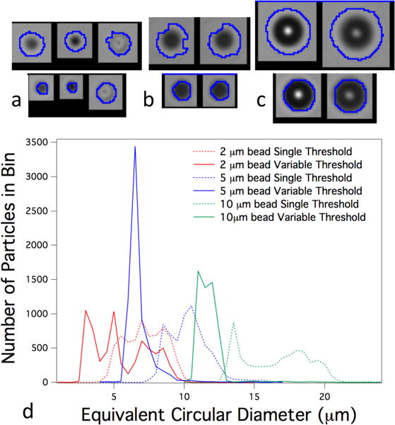
Results from polystyrene beads using variable thresholding and single threshold methods. In (a–c) particle boundaries as a result of image processing are shown: upper row shows images processed using single threshold, lower row shows the same images processed using variable threshold. Nominal bead size is (a) 2 μm, (b) 5 μm, and (c) 10 μm. (d) Number of particles as a function of equivalent circular diameter, sorted by size bins of 0.5 μm width. Nominal bead size and process method are as shown in the legend.

Table 2.

Summary of results on calibration beads.

Nominal Bead Size	Material	Solution refractive index at wavelength 589 nm	Single threshold average diameter (μm)	Variable threshold average diameter (μm)
2	Polystyrene	1.33	7.5	5.8
5	Polystyrene	1.33	10.7	7.0
10	Polystyrene	1.33	16.8	12
4	Silica	1.33	10.6	8.2
4	Silica	1.43	4.9	4.7
6	Silica	1.33	12.9	10.0
6	Silica	1.43	8.7	6.4

To test how the algorithm behaves when particles have a low contrast with respect to the liquid, we performed measurements on 4 μm and 6 μm silica beads with refractive indices of 1.44 and 1.42, respectively, in solutions of varying index of refraction. The images of particles were captured using flow instrument B. Images were processed using a direct subtraction of the particle frames from the background, equivalent to a ‘dark only’ pixels. This is consistent with the processing used in the software included with instrument B. As with Figure 4, the data was sorted into size bins. Figure 5a shows the bin populations for the two bead sizes for samples formulated in water (index of refraction, n = 1.33). Just as with the results in Figure 4, the single threshold method oversizes the beads by more than a factor of two as a result of the halo. The variable threshold data are substantially shifted to smaller size with a narrower size distribution for the 6 μm beads. When the index of refraction of the liquid is increased to 1.43, the particles have much less contrast with the background since this is closer to the refractive index of the silica particles themselves. As a result, the halo that would appear around such particles fades to a level that is closer to the threshold. As a result, the peaks for the data processed with a single-threshold shift to lower size as is evident in Figure 5b. For the 6 μm beads, the variable threshold results are shifted to even smaller size, now approximating the nominal size of the bead. For the 4 μm beads, the images have so little brightness relative to the background that the variable threshold algorithm has nearly “bottomed out.” Only 285 of 1253 analyzed particles were reanalyzed with a new threshold, and of these 219 were analyzed with a slightly higher threshold (11). Since the number of detected particles is conserved by the variable threshold method compared to the single threshold method, the peaks for the two methods for the 1.43 index case nearly overlap. The results on the silica particles demonstrates the variable threshold algorithm can more accurately size high contrast particles while detecting low contrast particles as effectively as a single, low-threshold detection algorithm.

Figure 5.

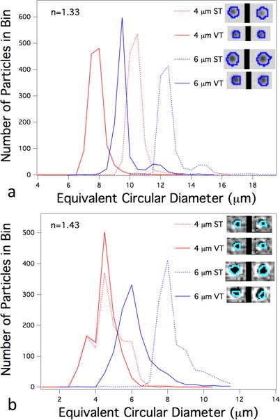
Results from silica beads in two fluids of different index of refraction: (a) n = 1.33 and (b) n = 1.43. Inset shows two image examples from each bead size/index of refraction combination.

Microfabricated rods were used to show the effect of image processing on elongated morphologies. Elongated morphologies may be present in a sample of protein aggregates, mixed in with less elongated morphologies, with all particles assigned an ECD by the instrument. This test shows the effect on reported ECDs of the boundary detection algorithm. Imaging was done using Instrument A. Figure 6a shows the images with overlays for single threshold (upper row of images) and variable threshold (lower row). Figure 6b shows the bin populations for the two methods, both for light and dark pixels included (absolute value subtraction of images from background), and for dark only (subtraction of images from background). The average of the ECD for single threshold processing with light and dark pixels included was 21.7 μm, in good agreement with the instrument reported result of 21.3 μm⁸. The variable threshold processing produces an average ECD of 17.1 μm. Note that if dark only pixels were considered in the analysis, the respective average ECD’s are 17.6 μm and 16.0 μm, approaching the ECD of 13.4 μm measured by electron microscopy for these rods. Figure 6c shows the results for aspect ratio obtained after processing the images with the same options as Figure 6b, showing that the processing method strongly affects the reported shape parameter.

Figure 6.

Results from microfabricated rods. (a) Images with overlays processed by (upper row) single threshold and (lower row) variable threshold algorithms. (b) Number of particles as a function of equivalent circular diameter, sorted by size bins of 1 μm width. (c) Number of particles as a function of aspect ratio.

Finally, the variable threshold algorithm was tested on a sample of protein aggregates. Along with the wide distribution in size, protein aggregates appear in microscope images with a distribution of particle brightness relative to the background. Figure 7a shows an example from data acquired using Instrument A with both light and dark pixels included. In this plot, particles detected by the starting low threshold (=8) were sorted according to the maximum gray value within each particle’s boundary just as in the method indicated in Figure 2. The distribution is roughly exponential. The variable threshold algorithm will analyze particles within each maximum gray value with a different threshold, as outlined earlier. Figure 7b shows a scatter plot of maximum gray value vs ECD as analyzed for a single threshold. It is interesting to observe that, while there is a correlation of particle size with maximum gray value, there is a considerable degree of variation.

Figure 7.

Results from IgG aggregates. (a) Number of particles as a function of maximum gray value. (b) Scatter plot of maximum gray value vs. particle equivalent circular diameter as evaluated using single threshold processing at threshold=8.

The results of analyzing the protein aggregates by the two methods are shown in Figure 8. Figure 8a is a selection of particles analyzed by a fixed threshold (upper row) and the variable threshold method (lower row). As with the beads and rods, the variable threshold overlays form a tighter boundary for the particles with greater contrast in the image. Figure 8b shows the results using fixed threshold values of 8, 12, 16, and 20 as well as the variable threshold, where the value of 8 was chosen as the starting threshold value. The particles were sorted into size bins of 0.5 μm. It is clear that for fixed threshold analysis, higher threshold values result in lower particle counts. As mentioned earlier, the variable threshold algorithm conserves the particle number when compared to the single threshold analysis for the starting threshold. For particles below 5 μm, the variable threshold method reports more particles than the value 8 threshold results—this effect is due to the tightening of particle boundaries by the variable threshold method resulting in more small particles. For particles above 5 μm, the variable threshold reports fewer particles and the trace crosses the traces from fixed thresholds of higher values until following closely the results for fixed threshold 20 for particles larger than 10 μm. This corresponds with the correlation between large size and maximum gray value in Figure 6b. Also plotted in Figure 8b is an example of a recently published correction algorithm applied to the fixed threshold=8 data to account for the combined effects of diffraction, out-of-focus effects, and the translucent nature of protein aggregates.¹⁷ The correction is applied to ECD values for each particle. The correction was based on operation of the instrument with settings of threshold=8 for light pixels and threshold=12 for dark pixels. To obtain the correction parameters, a calibration was performed with silica beads suspended in water-glycerol mixtures. Figure 8c shows the same data plotted in cumulative format. In Figure 8d the aspect ratio distributions reported by the two algorithms are plotted. While the results are quite similar, there is consistently a slightly higher number of aggregates with aspect ratios less than 0.5 that is returned by the variable threshold method.

Figure 8.

Results from IgG aggregates. (a) Images with overlays processed by single threshold=8 (upper row) and variable threshold (lower row) algorithms. (b) Number of particles as a function of equivalent circular diameter, sorted by size bins of 0.5 μm width for four values of fixed threshold (8,12,16,20),variable threshold and adjusted result calculated from fixed threshold 8 (c) Cumulative number of particles as a function of equivalent circular diameter, sorted by size bins of 0.5 μm width. (d) Number of particles as a function of aspect ratio.

Figure 9 illustrates the effect of changing focus on the determination of the particle boundaries by the two methods, using a standard microscope instead of a flow imaging instrument. In this figure, a single protein aggregate is photographed at a series of lens-sample distances, with the interval between images set at 5 μm. As in previous figures, the upper row of images depicts the boundaries set by a fixed threshold, while the lower row depicts the boundaries set by the variable threshold algorithm. As the particle comes into focus in the center image, the brightness increases, while the spatial extent of the particle diminishes. For this particle, the fixed threshold method picks up the outer blurred boundaries for when the particle is out of focus, resulting in a larger reported area for a particle out of focus. The variable threshold method sets a lower threshold for an image that is out of focus and a higher threshold for when the particle is in focus. This results in less change in reported area when the particle focus changes.

Figure 9.

Single IgG aggregate photographed at different focus distances. Images obtained with Leica DMRX at a magnification of 20×. Images are all of the same particle taken with a translation of the objective by 5 μm between images. Upper row shows images processed by single threshold, and lower row shows the identical images processed by the variable threshold algorithm.

DISCUSSION AND CONCLUSIONS

The variable threshold algorithm enables tighter boundaries to be defined for detected particles compared to the use of a single threshold, without the risk of losing particles by setting a fixed threshold at a high value. The method has several advantages. First, there is no requirement to guess the appropriate threshold to use for a measurement of a particular sample. This should simplify operation and can help improve comparisons between measurements taken on the same sample by different operators or by different instruments. In addition, the quandary over whether to change threshold settings on instruments like Instrument A when calibration particles are tested is eliminated. Second, the method should allow for improved measurements when different types of particles are present in the same sample. Third, with the improved values for particle size, particle counts will be more accurate. For example, in Figure 8c, it is evident that there is a substantial difference in the cumulative counts for any size greater than 4 μm. Improved accuracy for larger particles (as shown in Figs. 4–6) is attained without any sacrifice in detection of very translucent particles. Fourth, with improved particle boundaries, there is the opportunity for better classification studies based on particle shape. The difference in aspect ratio results for the rods in Figure 6c suggests that elongated particles will be more clearly separated from round particles.

Using the computer described in Materials and Methods, the algorithm was able to process 890 frames with 48605 particles in 75 s yielding an approximate frame rate of 12 fps. This is on the scale of frame rates used for data acquisition on commercial instruments. It should be noted that the ImageJ environment is not ideally suited for real-time use and it can reasonably be expected that considerable improvements in speed could be obtained by structuring the algorithm for real-time data analysis.

There are several further studies related to this method which may be considered. First is the role of “light” vs “dark” pixels. The results on rods in Figure 6 show that processing those images with only consideration of dark pixels results in improved accuracy. What properties of a particle indicate that the particle can be defined by its pixels that are darker than the background? Second, the variable threshold method makes possible lower starting threshold without sacrificing accuracy with brighter particles. In this work we used the identical baseline threshold commonly used for particle analysis in order to provide a clear comparison. Using a lower threshold may detect more particles, as long as the level is above the noise threshold for the CCD. This is related to the issue of particle transparency, which has been discussed in the literature^2,20. Thirdly, we would be able to implement additional improvements and corrections to the results obtained here. For example, a value of 0.5 times the maximum brightness was used to select the threshold for each image bin as a choice that gave good results. This number could be optimized by further studies. Variable thresholding makes use of an individual particle property—the maximum gray value—to help set a particle boundary. While it can reduce diffraction and out-of focus effects, it cannot eliminate them. The correction approach that was used in Figure 8 on the fixed threshold=8 data could be applied to variable thresholding data. This would require a calibration approach as in Ripple and Hu¹⁷ where the variable threshold method would be used in the data processing of calibrated beads in glycerol/water solutions. There are limitations on this correction however, as it requires knowledge of the detected particle properties. Making use of the perimeter for calculating an equivalent diameter may also help improve the comparability of the results to other methods.⁸ Other properties of the particle image, such as the gradient, may provide additional information. Modeling of how particles appear at different focal positions as in the images of Figure 9 and as was done by Dahl et al. for spray particles¹⁰ may prove useful to glean the maximum information out of a particle image for defining particle boundaries.

References

- 1.Corvari V, Narhi LO, Spitznagel TM, Afonina N, Cao S, Cash P, Cecchini I, DeFelippis MR, Garidel P, Herre A, Koulov AV, Lubiniecki T, Mahler HC, Mangiagalli P, Nesta D, Perez-Ramirez B, Polozova A, Rossi M, Schmidt R, Simler R, Singh S, Weiskopf A, Wuchner K. Subvisible (2–100 mu m) particle analysis during biotherapeutic drug product development: Part 2, experience with the application of subvisible particle analysis. Biologicals. 2015;43(6):457–473. doi: 10.1016/j.biologicals.2015.07.011. [DOI] [PubMed] [Google Scholar]
- 2.Zolls S, Gregoritza M, Tantipolphan R, Wiggenhorn M, Winter G, Friess W, Hawe A. How subvisible particles become invisible-relevance of the refractive index for protein particle analysis. J Pharm Sci. 2013;102(5):1434–1446. doi: 10.1002/jps.23479. [DOI] [PubMed] [Google Scholar]
- 3.Ripple DC, Montgomery CB, Hu ZS. An Interlaboratory Comparison of Sizing and Counting of Subvisible Particles Mimicking Protein Aggregates. J Pharm Sci-Us. 2015;104(2):666–677. doi: 10.1002/jps.24287. [DOI] [PubMed] [Google Scholar]
- 4.Sharma DK, Oma P, Pollo MJ, Sukumar M. Quantification and Characterization of Subvisible Proteinaceous Particles in Opalescent mAb Formulations Using Micro-Flow Imaging. J Pharm Sci-Us. 2010;99(6):2628–2642. doi: 10.1002/jps.22046. [DOI] [PubMed] [Google Scholar]
- 5.Brown L. Characterizing Biologics Using Dynamic Imaging Particle Analysis. Biopharm Int. 2011;24(8):S4–S9. [Google Scholar]
- 6.Sharma DK, King D, Oma P, Merchant C. Micro-Flow Imaging: Flow Microscopy Applied to Sub-visible Particulate Analysis in Protein Formulations. Aaps J. 2010;12(3):455–464. doi: 10.1208/s12248-010-9205-1. [DOI] [PMC free article] [PubMed] [Google Scholar]
- 7.Lee SY, Kim YD. Sizing of spray particles using image processing technique. Ksme Int J. 2004;18(6):879–894. [Google Scholar]
- 8.Cavicchi RE, Carrier MJ, Cohen JB, Boger S, Montgomery CB, Hu ZS, Ripple DC. Particle Shape Effects on Subvisible Particle Sizing Measurements. J Pharm Sci-Us. 2015;104(3):971–987. doi: 10.1002/jps.24263. [DOI] [PubMed] [Google Scholar]
- 9.Xu C, Shepard T. Digital Image Processing Algorithm for Determination and Measurement of In-Focus Spherical Bubbles. Proceedings of the Asme Fluids Engineering Division Summer Meeting; 2014; Symposia; 2014. [Google Scholar]
- 10.Dahl AL, Jorgensen TM, Larsen R. A Deformable Model for Bringing Particles in Focus. Comm Com Inf Sc. 2011;229:81–95. [Google Scholar]
- 11.Pedersen JS, Persson M. Unmasking Translucent Protein Particles by Improved Micro-Flow Imaging (TM) Algorithms. J Pharm Sci-Us. 2014;103(1):107–114. doi: 10.1002/jps.23786. [DOI] [PubMed] [Google Scholar]
- 12.Certain commercial instruments are identified to adequately specify the experimental procedure In no case does such identification imply endorsement by the National Institute of Standards and Technology.
- 13.Edelstein AD, Tsuchida MA, Amodaj N, Pinkard H, Vale RD, Stuurman N. Advanced methods of microscope control using μManager software. J Biol Methods. 2014;1(2) doi: 10.14440/jbm.2014.36. [DOI] [PMC free article] [PubMed] [Google Scholar]
- 14.Schindelin J, Arganda-Carreras I, Frise E, Kaynig V, Longair M, Pietzsch T, Preibisch S, Rueden C, Saalfeld S, Schmid B, Tinevez JY, White DJ, Hartenstein V, Eliceiri K, Tomancak P, Cardona A. Fiji: an open-source platform for biologicalimage analysis. Nat Methods. 2012;9(7):676–682. doi: 10.1038/nmeth.2019. [DOI] [PMC free article] [PubMed] [Google Scholar]
- 15.Collins TJ. ImageJ for microscopy. Biotechniques. 2007;43(1 Suppl):25–30. doi: 10.2144/000112517. [DOI] [PubMed] [Google Scholar]
- 16.Cavicchi RE. Flow Image Analysis. 2016 https://githubcom/usnistgov/FlowImageAnalysis 2016.
- 17.Ripple DC, Hu ZS. Correcting the Relative Bias of Light Obscuration and Flow Imaging Particle Counters. Pharm Res-Dordr. 2016;33(3):653–672. doi: 10.1007/s11095-015-1817-9. [DOI] [PubMed] [Google Scholar]
- 18.Kotarek J, Stuart C, De Paoli SH, Simak J, Lin TL, Gao YM, Ovanesov M, Liang YD, Scott D, Brown J, Bai Y, Metcalfe DD, Marszal E, Ragheb JA. Subvisible Particle Content, Formulation, and Dose of an Erythropoietin Peptide Mimetic Product Are Associated With Severe Adverse Postmarketing Events. J Pharm Sci-Us. 2016;105(3):1023–1027. doi: 10.1016/S0022-3549(15)00180-X. [DOI] [PubMed] [Google Scholar]
- 19.Zolls S, Weinbuch D, Wiggenhorn M, Winter G, Friess W, Jiskoot W, Hawe A. Flow Imaging Microscopy for Protein Particle Analysis-A Comparative Evaluation of Four Different Analytical Instruments. Aaps J. 2013;15(4):1200–1211. doi: 10.1208/s12248-013-9522-2. [DOI] [PMC free article] [PubMed] [Google Scholar]
- 20.Hu ZS, Ripple DC. The Use of Index-Matched Beads in Optical Particle Counters. J Res Natl Inst Stan. 2015;119:674–682. doi: 10.6028/jres.119.029. [DOI] [PMC free article] [PubMed] [Google Scholar]