Applying systems-level spectral imaging and analysis to reveal the organelle interactome

Abstract

The organization of the eukaryotic cell into discrete membrane-bound organelles allows for the separation of incompatible biochemical processes, yet the activities of these organelles must be coordinated. For example, lipid metabolism is distributed between the endoplasmic reticulum (ER) for lipid synthesis, lipid droplets (LDs) for storage and transport, mitochondria and peroxisomes for β-oxidation, and lysosomes for lipid hydrolysis and recycling^1–5. Organelle contacts are increasingly understood to be vital for diverse cellular functions^5–8. However, the spatial and temporal organization of organelles within the cell remains poorly characterized due to the inability of fluorescence imaging-based approaches to distinguish more than a few fluorescent labels in a single image⁹. Here we present a systems-level analysis of the organelle interactome using a multispectral image acquisition method that overcomes the challenge of spectral overlap in the fluorescent protein palette. We employed confocal and lattice light sheet (LLS)¹⁰ instrumentation and an imaging informatics pipeline of five steps to achieve mapping of organelle numbers/volumes/speeds/positions and dynamic inter-organelle contacts in live fibroblast cells. We describe the frequency and locality of two-, three-, four-, and five-way interactions among six different membrane-bound organelles (ER, Golgi, lysosome, peroxisome, mitochondria and LD) and show how these relationships change over time. We demonstrate that each organelle has a characteristic distribution and dispersion pattern in three-dimensional space and that there is a reproducible pattern of contacts among the six organelles, impacted by microtubule and cell nutrient status. These live-cell confocal and LLS spectral-imaging approaches are applicable to any cell system expressing multiple fluorescent probes, whether in normal conditions or when cells are exposed to disturbances such as drugs, pathogens or stress. This methodology thus offers a powerful new descriptive tool and source for hypotheses about cellular organization and dynamics.

To explore the spatiotemporal coordination among organelles, COS-7 cells were transfected to express fluorescent proteins targeted to lysosomes, mitochondria, ER, peroxisomes, and the Golgi, and incubated with a dye to label LDs (Extended Data Fig. 1a). Images were acquired using a laser scanning confocal microscope equipped with a spectral detector (Extended Data Fig 1b), and after applying a linear unmixing (LU) algorithm (Extended Data Fig. 1c–f) the six fluorophores could be separated into distinct compartments (Fig. 1a). Time-lapse images of single z-planes acquired every 5 seconds revealed the dynamics of all six labelled organelles within single cells (Video 1). These images were then processed using an imaging informatics pipeline for quantitative analysis of inter-organelle contacts (Extended Data Fig. 1g).

Figure 1. Live-cell, 6-colour confocal microscopy to characterize the organelle interactome.

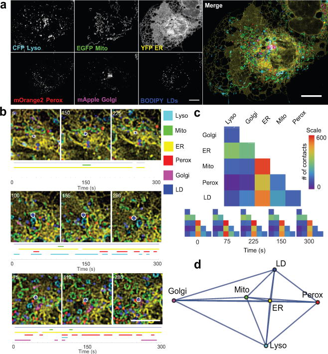
(a) Micrographs of a COS-7 cell expressing LAMP1-CFP, mito-EGFP, ss-YFP-KDEL, mOrange2-SKL, and mApple-SiT, and labelled with BODIPY 665/676. Micrographs are representative of 10 cells captured. (b) LDs (outlined in white) were tracked, and their interorganelle contacts mapped. A blue line indicates that the LD was successfully tracked, while coloured lines indicate that the LD was within 1 pixel (97 nm) of the indicated organelle at the specified time point. Numbers on the micrographs represent time (s). For more examples, see Extended Data Fig. 2. (c) Top: Matrix representation of the organelle interactome. The absolute numbers of organelle contacts in a single cell at a single time point are displayed as a graphical half matrix. Each row in the matrix represents the number of organelle contacts with each target organelle (columns), and is colour coded from 0 to 600. Bottom: Organelle interactome over time. Each half matrix represents the organelle interactome in a single cell at a specific time point. (d) Network representation of the organelle interactome in all ten cells. All nodes (organelles) are connected and the length of the edges connecting two nodes represents the inverse of the number of contacts between those two organelles. Mito, mitochondria; perox, peroxisomes; lyso, lysosomes. Scale bars, (a) 10 μm, (b) 5 μm.

We tracked individual LDs and mapped their contacts with other organelles over time. Maps of three different LDs revealed near continuous contacts with ER, the major site of lipid synthesis, but transient/heterogeneous contacts with all other organelles (Fig. 1b and Video 2). Histograms of LD-organelle contact duration revealed a higher fraction of long-lived LD-ER contacts (Extended Data Fig. 2a). Maps of LDs in a single cell further revealed that LDs were frequently associated with multiple organelles at the same time, and that some LDs associated with all five other organelles over the 300 second imaging period (Extended Data Fig. 2b), suggesting promiscuous exchange of lipids between LDs and other compartments.

We next characterized the number and pattern of contacts between all potential organelle pairs (i.e., 15 pairs, Fig. 1c). A matrix analysis of organelle interactions in a single cell (Fig. 1c, top panel) revealed that different organelle pairs showed different frequencies of contacts. Despite the transient nature of individual organelle contacts (Fig. 1b) the overall pattern of organelle interactions was stable over five minutes (Fig. 1c, bottom panel, Extended Data Fig. 3). This pattern of organelle contacts was consistent across ten cells (Extended Data Fig. 3). These results suggest that a conserved organelle interactome co-exists with a highly dynamic pattern of individual organelle contacts, with the ER acting as the central node in the organelle interactome network (Fig. 1d).

We quantified the fraction of globular organelles (LDs, peroxisomes or lysosomes) that made contacts with any of the other labelled organelles (Fig. 2a). Each of the globular organelles had a characteristic interaction repertoire. For example, 85% of LDs made contact with the ER. The second most common interaction partners for LDs were the mitochondria (21%) and Golgi (15%), while 10% of LDs contacted lysosomes or peroxisomes. We validated our six-colour imaging method to ensure that cell labelling and image acquisition parameters did not perturb organelle contacts (Extended Data Fig. 4a–b), and that our measurements were robust to errors in defining the edges of organelles (Extended Data Fig. 4c–d).

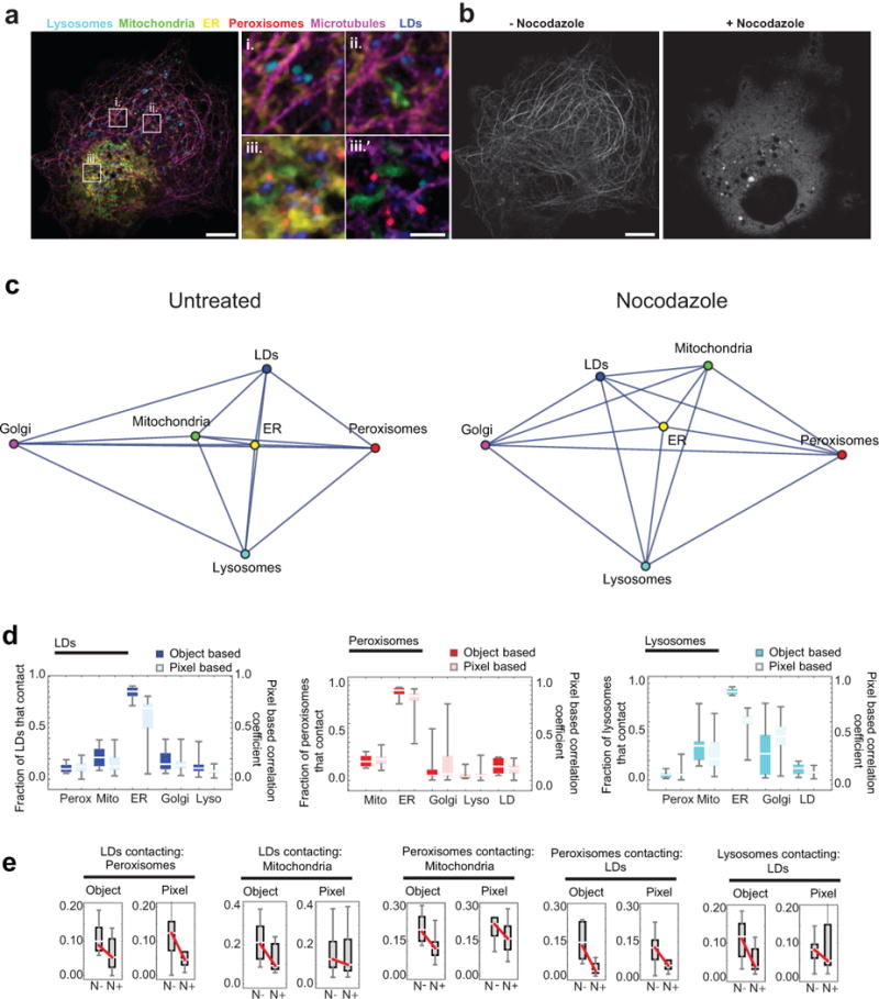
Figure 2. The organelle interactome depends on an intact microtubule cytoskeleton.

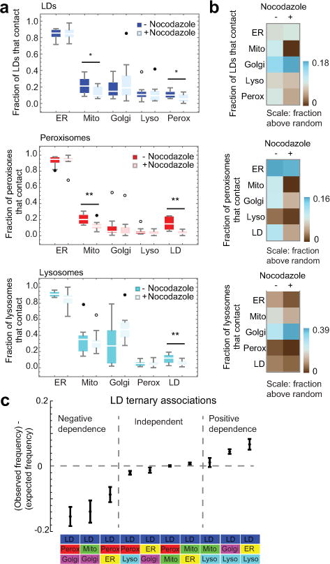
(a) Box whisker plots showing the median fraction of LDs, peroxisomes or lysosomes contacting each of the other labelled compartments in control (-Nocodazole) or nocodazole-treated (+Nocodazole) COS-7 cells. While the total number of contacts between two populations of organelles was, by definition, the same, the fractions of each of the populations in contact were not always symmetric because some individual organelles made simultaneous contact with two or more organelles of the same type. (b) Heat map comparison of control and nocodazole-treated cells to computer models of cells with random organelle distributions. The mean values for each interaction were calculated, then the mean value for random associations was subtracted, to give the frequency of associations above random for each binary organelle interaction in the absence or presence of nocodazole. (a-b) n = 11 (nocodazole-treated) or n = 10 (untreated) cells from two experiments. * 0.05 > p < 0.01, ** p < 0.01 (unpaired two-tailed t-test). (c) Plot of observed LD ternary contact frequency minus expected frequency, assuming the probabilities of all contacts are independent of each other. n = 10 cells. Error bars represent standard error of the mean (s.e.m).

Given the primary role of microtubules in organizing organelles and inter-organelle contacts (Extended Data Fig. 5a)^11–14, we next examined how the observed pattern of organelle interactions was affected by microtubule disruption by nocodazole treatment (Extended Data Fig. 5b). Except for the fraction of lysosomes contacting Golgi, which increased after nocodazole treatment, the fractions of most organelles making contacts with other organelles decreased after nocodazole treatment and were more similar to those observed in computer models with randomly placed organelles (Fig. 2a–b, Extended Data Fig. 5c and Video 3). This indicated that microtubules play a vital role in establishing and maintaining multiple types of inter-organelle contacts. We confirmed these results using a pixel-based co-localization analysis (Extended Data Fig. 5d–e)¹⁵.

We tested the effect of starvation or excess fatty acids on LD-organelle contacts (Extended Data Fig. 6). In response to starvation, the fraction of LDs contacting mitochondria increased, consistent with the role of these contacts in transferring fatty acids from LDs to mitochondria for β-oxidation^11,16. LD contacts also increased with lysosomes. This could aid in restoring starvation-depleted fatty acid reserves within LDs, since lysosomes release fatty acids derived from autophagy of cell membranes¹⁶. In response to excess oleic acid, the fraction of LD-peroxisome contacts decreased while that of LD-lysosome contacts increased. These changes may reflect increased lysosomal digestion of LDs under excess oleic acid conditions¹⁷.

We next measured the frequency of contacts among LDs and two other different organelles under complete media conditions. We compared the frequency of these tripartite contacts to that expected if all organelle contacts are independent of each other (Fig. 2c). We found three regimes existed: some tripartite interactions occurred at the expected frequency; some occurred less than expected; and, others occurred more frequently. The observed higher than expected frequency of LD contacts with ER and lysosomes, and of LD contacts with Golgi and lysosomes, could reflect the known coordination of lipid trafficking among these organelles¹.

To acquire three-dimensional images of organelles in live cells with high spatial and temporal resolution, we next developed a LLS implementation of multispectral imaging using an excitation-based LU approach (Extended Data Fig. 7a–c). This resulted in 3-D images (Fig. 3a, Extended Data Fig. 7d–e) and 4-D videos (Video 4) in which six organelles were distinguished. The mean number, mean volume, total volume per cell of the organelles, and total cell volume in these images, as well as the speed of globular organelles from confocal images, are reported in Extended Data Table 1. These measurements revealed that the ER occupies approximately 37 times the volume of the Golgi and 9 times the volume of the mitochondria; the numbers of LDs, peroxisomes and mitochondria each ranged between ~150–190 per cell; and the maximum speed of movement of lysosomes was twice that of LDs and peroxisomes.

Figure 3. Live-cell, 6-colour 4D LLS microscopy to characterize organelle distribution in space and time.

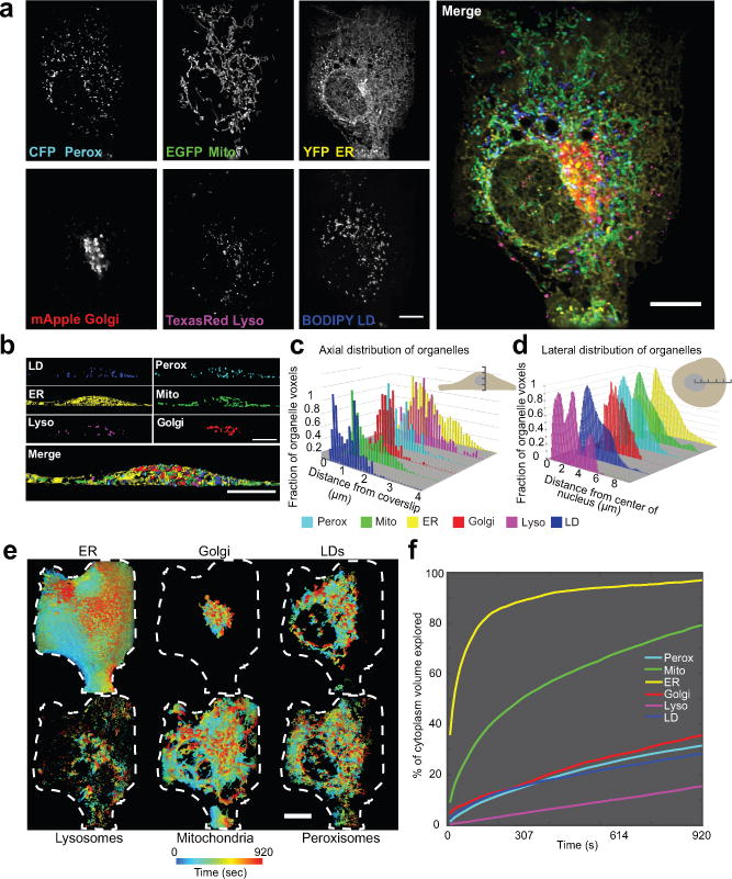
(a) Maximum intensity projections of a COS-7 cell expressing CFP-SKL, mito-EGFP, ss-YFP-KDEL, and mApple-SiT, and labelled with Texas Red dextran and BODIPY 665/676. (b) XZ images of segmented LLS images. (c-d) Distributions of organelles in the axial (c) and lateral (d) dimensions of a single COS-7 cell, representative of 10 cells captured. (e) Organelle dispersion in the cell over time. Voxels are colour coded according to the time that an organelle last occupied that voxel. Shown are 2-D projections where only the outer shell of the volume is visible. Cell was masked using the total dispersion of the ER as a proxy for the cell boundary. Dashed white lines represent the 2-D projected outline of the cell generated from the mask. See Video 5 to explore the volume in depth. (f) Dispersion analysis. The summed fractional cytoplasmic volume (excluding the nucleus) occupied by each organelle is plotted as a function of time. Scale bars, (a, e) 10 μm, (b) 5 μm. Micrographs are representative of 10 cells.

COS-7 cells displayed characteristic organelle distribution patterns in both the lateral and axial dimensions (Fig. 3b–d). As shown for one cell, in the lateral dimensions, the ER had the widest distribution and Golgi the narrowest (Fig. 3d). In the axial dimension, Golgi displayed a narrow distribution in the centre of the cell, while ER, LDs, mitochondria and peroxisomes were localized throughout the cell, with concentrations near both the dorsal and ventral surfaces of the plasma membrane (Fig. 3c). These patterns were qualitatively consistent across the ten cells observed.

To map out total cytoplasmic volume explored by each organelle over time, we made time dependent volume renderings of our 3-D images (Fig. 3e, Video 5). At time 0, the ER occupied just over 25% of the cell volume, excluding the nucleus, but quickly explored over 97% of it within 15 min, whereas lysosomes occupied a small fraction of the cell volume and explored just over 15% over the same time period (Fig. 3f). The Golgi remained largely peri-nuclear, but traced through a considerable volume. The ER’s exploration of virtually the entire cytoplasmic volume may explain its ability to rapidly sense and respond to overall changing cellular needs⁵.

We observed complex organelle morphologies, such as LDs contacting mitochondria, ER, or Golgi (Fig. 4a). These morphologies were especially striking when all six channels were viewed at once (Fig. 4b). Quantification of organelle interactions in LLS images yielded comparable results to those obtained by single z-plane confocal microscopy (Extended Data Fig. 8a), with the ER showing the highest contact rate. The preponderance of organelle-organelle contacts occurred in the juxtanuclear region (Fig. 4c). The exception to this was the fraction of the population of LDs, peroxisomes or lysosomes contacting ER, which was similar in the juxtanuclear region to elsewhere in the cell (Fig. 4c). As with our confocal data, we ensured that image acquisition parameters did not perturb organelle contacts and that our measurements were robust to errors in segmentation (Extended Data Fig. 8b–d). We also compared object-based and pixel-based analysis methods, again obtaining complementary results (Extended Data Fig. 9).

Figure 4. LLS analysis of the organelle interactome in 3D.

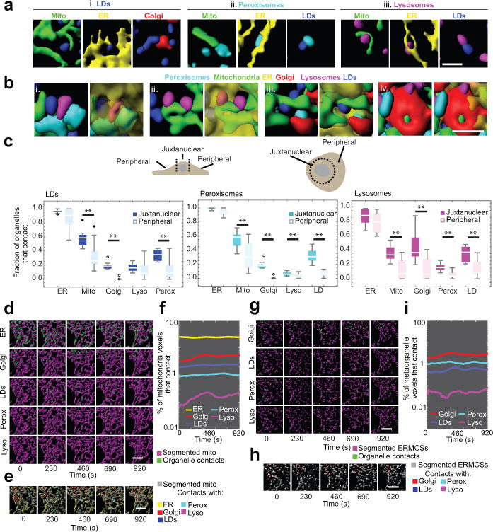
(a) Examples of LD- (i.), peroxisome- (ii.) and lysosome- (iii.) interorganelle contacts in segmented LLS images. For clarity, only two channels are shown. (b) Examples of complex interorganelle contacts and organisation in segmented LLS images. (i.-iv.) The ER (transparent yellow) is shown in the right panels only. (c) Box whisker plots showing the median fraction of LDs, peroxisomes, or lysosomes contacting each of the other labelled compartments in the juxtanuclear or peripheral regions of the cell. n = 10 cells. ** p < 0.01 (paired two-tailed t-test). (d) Fields of view from volume rendered images of mitochondria (magenta) and sites of mitochondrial contact with five other organelles (green) in LLS images at discreet time points. (e) Fields of view from volume rendered images of mitochondria (grey) and sites of mitochondrial contact with all five other organelles. (f) Percentage of segmented mitochondria voxels that contact other organelles over time in the cell shown in (d-e). (g) Fields of view from volume rendered images of ERMCSs (magenta) and sites of contact with four other organelles (green). (h) Fields of view from volume rendered images of ERMCSs (grey) and sites of contact with all five other organelles. (i) Percentage of ERMCS voxels that contact other organelles over time in the cell shown in (g-h). Scale bars: (a-b) 2 μm, (d-e, g-h) 5 μm. Micrographs are representative of 10 cells captured.

We next visualized individual organelle contacts with mitochondria in three dimensions over time (Fig. 4d and Video 6) and as a group (Fig. 4e and Video 7). This revealed that multiple organelle types simultaneously interact with mitochondria, with the ER being the most prominent interacting partner, followed by Golgi and LDs (Fig. 4f). We then treated the extensive interaction sites between ER and mitochondria (i.e., ER mitochondria contact sites, ERMCSs) as a ‘metaorganelle’, visualizing its contacts with other organelles (Fig. 4g–h and Video 8). The ERMCS metaorganelle made most contacts with Golgi, followed by peroxisomes and LDs (Fig. 4i). ERMCS association with Golgi could be required for efficient cholesterol transport between ER, mitochondria and Golgi¹⁸.

Our visualization and quantification of dynamic contacts between six different organelles will allow targeted research on the molecular mechanisms that guide these relationships. We anticipate the use of live-cell multispectral imaging in investigating organelle organization and interactions in cells exposed to drugs, pathogens, and other stressors, as well as during cell migration, division and differentiation. This approach should also be useful for identifying proteins that mediate or regulate contact site formation (e.g., tethers)¹⁹. Developments in making brighter and more photostable fluorescent proteins, as well as improvements in genome editing and computational tools for automated image analysis, should enable multispectral imaging approaches to discriminate even more than six molecular species over time in single cells.

Methods

Cell Culture and Transfection

COS-7 cells obtained from the American Type Culture Collection (CRL-1651) were maintained in Dulbecco’s modified eagle’s medium (DMEM, Life Technologies) supplemented with 10% foetal bovine serum (Corning), at 37 °C and 5% CO₂. For confocal imaging, cells were cultured in 10 μg/ml fibronectin (Millipore)-coated LabTek 8-well Chambered Cover glass dishes (ThermoScientific), and transfected with the following FPs, either alone or in combination: lysosomes were labelled with lysosomal-associated membrane protein 1 fused to CFP (LAMP1-CFP, G. Patterson, constructed as described for PA-GFP-lgp120²⁰); mitochondria were labelled with the mitochondrial targeting sequence of cytochrome c oxidase subunit VII fused to EGFP (mito-EGFP, A. Rambold); the ER was labelled with a fusion of the bovine prolactin signal sequence with YFP and a KDEL ER retention sequence (ss-YFP-KDEL, E. Snapp, constructed as described for ss-GFP-KDEL²¹); peroxisomes were labelled with mOrange2 fused to the peroxisome targeting sequence SKL (mOrange2-SKL); and the Golgi was labelled with mApple fused to the 15 N-terminal amino acids of sialylytransferase (mApple-SiT). For experiments shown in Extended Data Fig. 5a–b, mApple-SiT was replaced with mApple fused to the 10 C-terminal amino acids of microtubule associated protein 4 (mApple-MAP4-C10). Transfection was performed using Lipofectamine 2000 (Life Technologies), according to the manufacturer’s instructions. Briefly, cells were transfected in Opti-MEM (Life Technologies) with 50–200 ng of each plasmid and 0.5 μl Lipofectamine 2000/well. Cells were incubated in the transfection mixture for 6 h, and then the medium was replaced with standard culture medium. BODIPY 665/676 (50 ng/ml, Life Technologies) was added to the medium for 16 h prior to imaging and was present during imaging. Where indicated, cells were treated with 5 μM nocodazole (Sigma-Aldrich) on ice for 2 min, warmed to 37 °C, and imaged 1 h after the addition of nocodazole. For nutritional perturbation experiments, cells were incubated in Hanks’ balanced salt solution (HBSS, Gibco 14025) or complete medium supplemented with 300 μM oleic acid (oleic acid-albumin from bovine serum, Sigma-Aldrich) for 18 h prior to imaging. For LLS imaging, cells were cultured on 10 μg/ml fibronectin-coated 5 mm coverslips, and transfected with CFP-SKL (P. Kim, constructed as described for RFP-SKL²²), mito-GFP, ss-YFP-KDEL, and mApple-SiT as described above. BODIPY 665/676 (50 ng/ml, Life Technologies) was added to the medium for 16 h prior to imaging and was present during imaging. Texas Red dextran (10,000 MW, 10 μg/ml, Life Technologies) was added to the medium for 14 h, washed 3 times, and chased for 2 h in standard culture medium (including BODIPY 665/676) prior to imaging.

Image Acquisition and Unmixing

Laser Scanning Confocal

Images were acquired on a Zeiss 780 laser confocal scanning microscope equipped with a 32-channel multi-anode spectral detector (Carl Zeiss) using a 63×/1.4 NA objective lens, at 37 °C and 5% CO₂. All fluorophores were excited simultaneously using 458, 514 and 594 nm lasers and a 458/514/594 nm main beam splitter, and images were collected onto a linear array of 32 photomultiplier tube (PMT) elements in lambda mode at 9.7 nm bins from 468 to 687 nm. Images were acquired with 5.0 s intervals between frames for 60 frames. We acquired images of cells labelled with single fluorophore reporters (each of the six reporters used to label multiply-labelled cells) using the same image acquisition settings as for multiply-labelled cells (same laser power and master gain settings). Spectra were defined using images from singly-labelled cells, and images from multiply-labelled cells were subjected to LU using Zen software (Carl Zeiss). To estimate the error in assigning a pixel to the wrong organelle after unmixing, cells expressing single FPs or incubated with BODIPY only were subjected to image segmentation, then the mean pixel intensity for every pixel in the foreground was computed for each of the six fluorophores (Extended Data Fig. 1f). In all cases, the correct fluorophore intensity was at least an order of magnitude higher than any incorrectly assigned fluorophore. In general, with well-acquired reference spectra, the error in unmixing is assumed to be a result of noise in the image. For time-lapse imaging, a single frame was first acquired and subjected to LU, in order to ensure that the cell was expressing all five fluorescent proteins at roughly equal levels. As a general rule of thumb, for successful LU the intensity of the fluorophores in the sample should not differ by more than one order of magnitude. Approximately 5–10% of the transfected cells met this criteria, making them suitable for time-lapse imaging.

Unmixed images were then spatially deconvolved using Huygens software (Scientific Volume Imaging) using theoretical point-spread functions. In principal, spatial deconvolution could have been performed on the images before LU. Because hyperspectral images generally contain many more wavelength channels before unmixing than they do after unmixing (e.g., our confocal data set consisted of 26 spectral channels before unmixing and only six after), it may be computationally more efficient to perform LU on these data sets first, before applying a highly iterative spatial deconvolution procedure.

Lattice Light Sheet

The LLS instrument illuminates the specimen with an ultrathin light sheet derived from 2-D optical lattices¹⁰. The thinness of the sheet leads to high axial resolution while simultaneous illumination of the entire field of view permits imaging at hundreds of planes per second, leading to full 3-D live cell imaging of cells with near isotropic resolution. A recent implementation of spectral light sheet imaging utilized a diffraction grating to project dispersed light onto a camera, allowing fine sampling of emitted light across the visible spectrum, but still required scanning of the sample in two dimensions, y and z, making it relatively slow²³. To avoid this drawback, we adapted a LLS instrument for spectral imaging with a multispectral excitation- based approach (Extended Data Fig. 7). This obviated the need to scan in y, giving fast acquisition rates and allowed imaging at subcellular resolution over time.

Images were acquired on a custom LLS instrument¹⁰ equipped with a 25× 1.1 NA imaging objective and digital camera with a scientific complementary metal oxide silicon (sCMOS) sensor (Hamamatsu Orca Flash 4.0) and six solid state lasers (MPB Communications) emitting at 445, 488, 532, 560, 590 and 642 nm wavelengths. 3D image stacks of 140 planes per cell were acquired every 9.2 s for 100 time points, n=10 cells. Image stacks were acquired sequentially at each laser wavelength, with emission collected through a series of four interference filters (Semrock), which functioned to block excitation wavelength bands and transmit emission wavelength bands to the CMOS detector. These filters were a notch filter with transmission minima at 405, 488, 561 and 635 nm, a long pass filter with transmission edge at 442 nm, a notch filter with transmission minimum at 532 nm and a notch filter with transmission minimum at 594 nm. We acquired images of cells labelled with single fluorophore reporters using the same laser power and exposure time as for multiple-labelled cells. To estimate the error in assigning a pixel to the wrong organelle after unmixing, singly-labelled cells were subjected to image segmentation, then the mean pixel intensity for every pixel in the foreground was computed for each of the six fluorophores (Extended Data Fig. 7c). Lateral and axial resolution at each of the excitation wavelengths, measured as the FWHM intensities of 100 nm diameter beads, are as follows: 445 nm: 0.294 μm (lateral) × 0.649 μm (axial); 488 nm: 0.312 μm (lateral) × 0.666 μm (axial); 532 nm: 0.375 μm (lateral) × 0.731 μm (axial); 560 nm: 0.359 μm (lateral) × 0.771 μm (axial); 589 nm: 0.370 μm (lateral) × 0.789 μm (axial); and 642 nm: 0.370 μm (lateral) × 0.947 μm (axial).

LU was performed using a custom algorithm in Mathematica. Organic fluorophores including fluorescent proteins have characteristic emission and excitation spectra. When excited with different wavelengths of light, different fluorophores emit different numbers of photons based on their probability of absorbing a photon and transitioning to an excited state at that particular wavelength. The recording of differential emission intensities with different wavelengths thus approximates the excitation spectrum of each fluorophore and is revealed to be characteristic for each fluorophore (Extended Data Fig. 7b). Our excitation-based unmixing algorithm uses this excitation information as reference spectra, rather than using emission data. With LU, the observed spectrum at every pixel in a spectrally resolved digital image and the known spectra of the fluorophores present in the specimen can be treated as a system of linear equations of the general form:

$$\left\{\begin{array}{c}\begin{array}{c}{y}_1\\ y_2\end{array}\\ ⋮\\ y_q\end{array}\right\}=\left[\begin{array}{ccc}{m}_{1,1}& \dots & m_{p,1}\\ ⋮& \ddots & ⋮\\ m_{1,q}& \dots & m_{p,q}\end{array}\right]·\left\{\begin{array}{c}{x}_1\\ ⋮\\ x_p\end{array}\right\}+\left\{\begin{array}{c}\begin{array}{c}{n}_1\\ n_2\end{array}\\ ⋮\\ n_q\end{array}\right\}$$ 1

where the column vector with elements labelled y is the observed pixel spectrum, the matrix with elements, m are the known fluorophore spectra, the column vector with elements x are the abundances of all of the fluorophores used to label the specimen and the column vector with elements n is the noise in the observed spectrum. Equation 1 can be simplified as:

$$\mathbf{y}=\mathbf{M}·\mathbf{x}+\mathbf{n}$$ 2

the vector x is solved for with the method of least squares by applying an inverse or pseudo inverse operation to the matrix, M:

$$\mathbf{x}={({\mathbf{M}}^{\mathbf{T}}\mathbf{M})}^{-1}{\mathbf{M}}^{\mathbf{T}}\mathbf{y}$$ 3

In practice, a non-negativity constraint is usually imposed upon the solution for x and is not shown in this generalized expression. We implemented the least squares algorithm using the Mathematica optimization function, “FindMinimum” and included a non-negativity constraint. For computational efficiency, the unmixing problem was first solved without the non-negativity constraint. If all answers to x were positive, the solution was kept. If any of the elements of x were negative, the solution was discarded and the problem was solved a second time with the non-negativity constraint imposed. Before unmixing, images were corrected for chromatic aberration with a linear pixel transformation, using values derived from images of “tetra-spec” multi-labelled subresolution fluorescence beads (Life Technologies). After unmixing, images were spatially deconvolved using experimentally derived point spread functions for each excitation wavelength.

Image Analysis

Laser Scanning Confocal

Unmixed images were segmented in Mathematica using algorithmic, histogram based approaches for defining intensity thresholds. The optimal threshold values for all organelles except ER were determined using the Mathematica implementation of Otsu’s method²⁴. ER was segmented using a local threshold determined using the Mathematica function: LocalAdaptiveBinarize[]. Globular organelles were tracked using the TrackMate plugin (an ImageJ implementation of the linear assignment problem (LAP) tracking algorithm)²⁵. The segmented images and tracking data were then imported into Mathematica for organelle interactome analysis. We wrote a custom feature based colocalization analysis program. Because globular organelles were segmented in two different software environments (Mathematica for contact analysis and ImageJ for tracking), the segmented images were first merged in Mathematica before analysing contacts. Organelle contacts in confocal images were defined as an overlap or 3 or more contiguous pixels between segmented features, with the target feature dilated 1 pixel (equivalent to 97 nm). We recognize that this definition may lead to an overestimate of contacts, since the distance between membranes at membrane contact sites studied by electron microscopy has generally been reported in the range of 15–30 nm.²⁶ However, the maximum distance between membranes that allows for a functional interaction (such as for the transport of lipid molecules) is unclear, and may be even greater than 100 nm due to the long lengths of organelle-organelle tethering proteins.²⁶

For analysis of the organelle interactome, the first frames of segmented images of cells were analysed for regions of overlap between different organelles. The number of globular organelles that overlap with each of the 5 other organelles was then computed and compared to models of randomly distributed organelles within images of cells. To construct models, the segmented images of all five organelles not of interest were used as a base image upon which the model globular organelles of interest (either peroxisomes, lysosomes or LDs) were distributed using a random number generator for centroid coordinates. Parameters for the model images, e.g., number and size of globular organelles of interest, were derived from the measurements of segmented images of multi-labelled cells.

Network diagrams were constructed from the mean number of contacts for each organelle pair from all cells observed for each condition in Mathematica. The length of edges connecting all nodes was calculated as the inverse of the number of contacts between those two organelles—shorter edges means higher number of contacts. The six-dimensional network was then rendered as a diagram in 2-D space to minimize the global error in total edge length.

Lattice Light Sheet

Unmixed images were segmented and organelle contacts analysed using Imaris software (Bitplane). Segmentation was performed with the surfaces tool, using smoothing and background subtraction, and manual thresholding. Split touching objects was used for the globular organelles (LDs, peroxisomes, and lysosomes). Objects smaller than 10 voxels were excluded. Distance transformations were performed to calculate the distance between objects, and organelles with a minimum distance of 0 nm between edges were considered to be interacting. For analysis of juxtanuclear vs. peripheral organelle interactions, the region of the cell with a thickness greater than approximately 2 μm was considered juxtanuclear, and was masked manually. For analysis of organelle distribution in 3D, the centre of the nucleus was estimated visually.

Automated Pixel-Based Quantification of Organelle Co-localization

A custom MATLAB program was written to capture co-localizations among pixels in the thresholded images. This approach is useful in measuring interactions among organelles with variable and non-globular morphology that would otherwise be difficult to accurately characterize. Boundary regions for individual cells in each image were identified manually using ER as a marker for the full cell. Each channel image was median filtered using a 5-pixel support. An adaptive threshold was computed using Otsu’s method²⁴ and the images were binarized. Mathematical morphology²⁷ was used to fill in a two pixel radius around each object for co-localization measurements with a dilation operator. For each organelle image $I_{ox}$ we define the set of foreground pixels obtained from this processing as $P_{\mathit{Iox}}={\left\{\left(x,y\right)\right\}}_{\mathit{Iox}}$. The co-localization S between two organelle channels is then calculated from the normalized intersection cardinality,

$$D(I_{o1},I_{o2})=1-\frac{\left|P_{Io1}\mathrm{I}{P}_{Io2}\right|}{min(\left|P_{Io1}\right|,\left|P_{Io2}\right|)}.$$

S takes on values in the range [0,1]. S achieves a value of one when the organelles are perfectly co-located, that is when all the foreground pixels from the processed channel images intersect each other following the morphological processing, and a value of zero when organelles are not co-localized anywhere. These co-localization measures were computed between each organelle pair in each image frame, creating a six by six matrix that is symmetric, with zeros on the diagonal. The co-localization measures from each image frame were combined for each experimental condition to form a distribution of co-localization. The object-based contact analysis and pixel-based colocalization analyses are not expected to always yield similar results, as seen in Extended Data Fig. 5d. This is because the object based method measures the frequency of objects touching, whereas the pixel-based method measures the statistical similarity between different image channels. Object-based methods provide a reliable quantification of organelle contacts but require an assumption that the image segmentation faithfully identifies the edges of organelles. The pixel-based method used here to validate our object-based analysis does not require this underlying assumption regarding identification of organelle edges, nor does it answer the specific question: where do organelle edges make contacts with other organelle edges. The same pixel-based approach was applied to both 2-D confocal and 3-D LLS multi-channel time-lapse images. A software tool called LEVER 3-D²⁸ originally developed for characterizing neural stem cell interaction with blood vessels¹⁵ was used here to visualize the interaction between mitochondria and the other organelles (Fig. 4d–e), or the interaction between ERMCSs and other organelles (Fig. 4g–h).

Statistics

All statistical analyses (Student’s t-tests and Student’s paired t-tests) were performed in Mathematica. For all box whisker plots, the white line in the centre of each box represents the median value, the upper and lower edges of the boxes represent the 75^th and 25^th quantile of the data respectively and the upper and lower fences represent the 95% confidence level of the distribution. Closed circles represent near outliers defined as points beyond 3/2 times the interquantile range from the edge of the box while open circles denote far outliers defined as points beyond 3 times that range.

To assess the variance between cells across time in the number of organelle contacts (as in Fig. 1c and Extended Data Fig. 3a), we performed an analysis of variance (ANOVA). The 15 element vector of each frame was normalized to a sum of 1 and then averaged across time, and a correlation distance was computed between each image frame-15-element vector and the average vector. The variance between frames as determined by a correlation distance from the average vector over the 60 image frames was then evaluated as a measure of within-cell temporal variation of the organelle interactome. The variance between cells was evaluated in the same way, with each cell being represented by their average vector. The results show that the variance between cells is significantly larger than the variance within an individual cell across time (p<1×10^−37). To quantify the similarity of organelle contact patterns between cells, we performed a cluster analysis using the correlations between organelle associations shown in Extended Data Fig. 3b. The gap statistic^29,30 is a widely used technique for estimating the number of clusters in a dataset. The gap statistic compares the average intra-cluster dispersion of the given data to that of uniformly distributed randomly generated data on the same range, and picks the number of clusters as maximizing the improvement of the given data compared to the random data. For the organelle association data in Extended Data Fig. 3a, the gap statistic found a single cluster in the data, with no meaningful differences to separate the organelle associations for the ten cells.

Extended Data

Extended Data Figure 1. Strategy for 6-colour labelling, image acquisition and analysis (confocal).

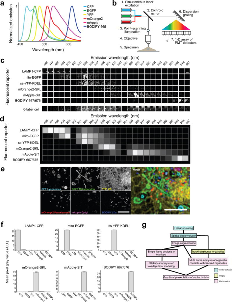
Fluorescence spectral imaging has emerged as a technology that allows many different spectrally variant fluorescent markers to be distinguished in a single sample³¹. The most widely used approach for computational analysis of spectral images, called linear unmixing (LU), involves a matrix inverse operation to find the best fit of known fluorophore spectra to that of the recorded spectrum at every pixel in a digital image⁹. Although this and other multispectral approaches have been used in commercial instruments to distinguish multiple combinations of organic dyes in fixed microbes^32,33 and fixed neuronal tissue³⁴, its application to multi-labelled cells and their quantitative analysis remains underdeveloped in live cell experiments. (a) Published emission spectra for the fluorophores used in confocal experiments: CFP³⁵, EGFP³⁵, YFP³⁵, mOrange2³⁵, mApple³⁶ and BODIPY 665/676³⁷. (b) Schematic of the hardware used for 6-colour confocal microscopy. The specimen was excited using three lasers simultaneously, by point-scanning illumination. Emitted light was collected by a linear array of detector elements after being dispersed by a reflective dispersion grating. (c) To derive the values for the known fluorophore matrix, images of singly labelled cells were acquired at each wavelength and under the same acquisition conditions used to acquire images of 6-label cells. Intensity values centred at 512 nm and 591 nm were zero for all cells because these detector elements were blocked to prevent scattered laser excitation light from reaching the detector. (d) Graphical representation of the unmixing matrix. The normalized intensity values at each wavelength range from 0 to 1. (e) Zoom-up of a region of the cell shown in Fig. 1a. Scale bars, 5 μm. Micrographs are representative of 10 cells captured. (f) Plots of mean pixel intensity values for all 6 fluorophores in every pixel in singly labelled cells that were segmented as foreground. Cells were singly labelled with LAMP1-CFP, mito-EGFP, ss-YFP-KDEL, mOrange2-SKL, mApple-SiT, or BODIPY 665/676. n = 87,307 pixels from one cell (CFP), 5,933 pixels from one cell (EGFP), 84,127 pixels from one cell (YFP), 2,711 pixels from one cell (mOrange2), 11,804 pixels from one cell (mApple), 3,332 pixels from one cell (BODIPY 667/676). Error bars represent s.e.m. A.U. = Arbitrary Units. (g) Imaging-informatics pipeline for quantitative analysis of organelle contacts. 32-channel micrographs of samples were subjected to pixel-based LU and spatial deconvolution algorithms, resulting in 6-channel unmixed images. These images were segmented to generate features, and contacts between features (within 1 pixel, 97 nm) were analysed in single frames. Alternatively, globular organelles were tracked and their contacts with segmented features analysed over multiple frames. The pipeline is modular and involves five major components: pixel-based LU of raw image data; spatial deconvolution; segmentation of organelles to generate features; particle tracking of globular organelles over time; and integration of track data with segmented image data to identify organelle contacts between the labelled organelles. The first four modules are implemented in existing software packages, either commercially available (Zeiss Zen and Huygens software) or freely available (histogram based segmentation algorithms and TrackMate plugin in ImageJ for particle tracking)^38,39. For the final component of the pipeline we developed an image analysis program on the Mathematica platform (available for downloading at http://organelle-interactome.sourceforge.net) that identifies feature-based colocalization.

Extended Data Figure 2. LD-organelle contact duration and dynamics.

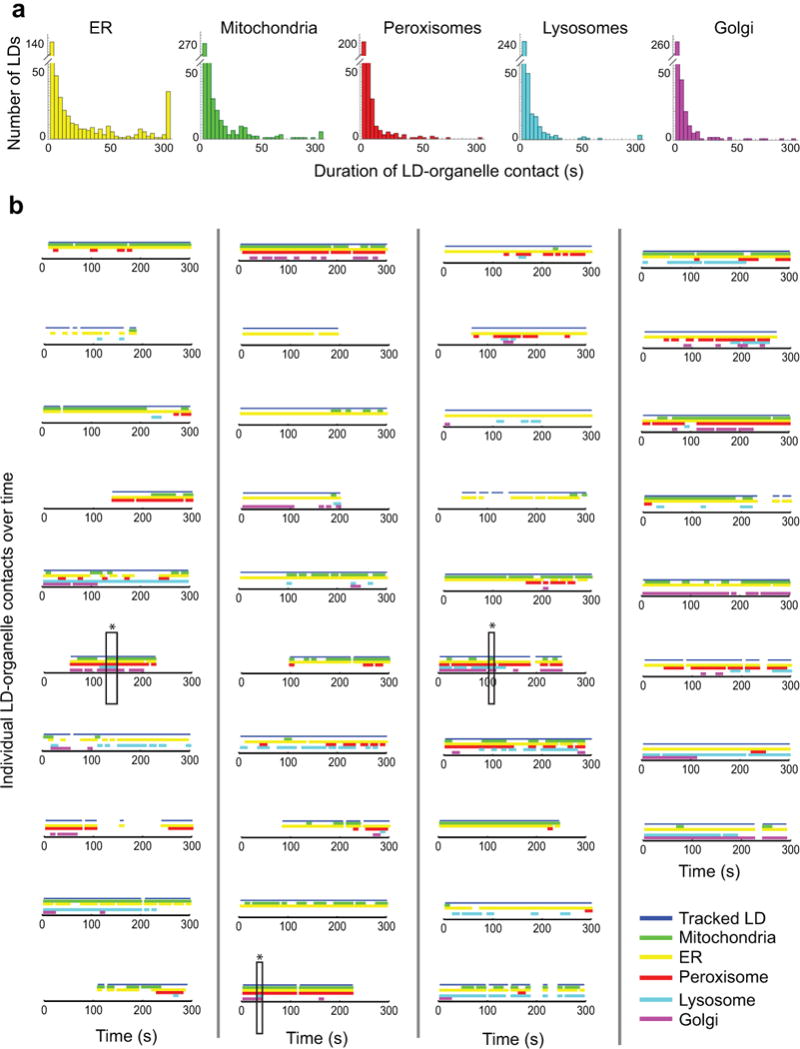
(a) Histograms showing the duration of LD-organelle contacts in time lapse images of a single cell, acquired and analysed as described in Fig. 1b. n = 480 LD contact events from one cell. (b) All the LDs in a single cell were tracked, and their interorganelle contacts mapped with time. A blue line indicates that the LD was successfully tracked at the specified time point. Coloured lines indicate that the tracked LD was within 1 pixel (97 nm) of the following organelles at the specified time point: green, mitochondria; yellow, ER; red, peroxisome; cyan, lysosomes; magenta, Golgi. Tracks are sorted according to LD speed, from fastest to slowest. Only LDs that were tracked for at least 25 out of 60 frames are included. Boxes marked with stars indicate examples where a single LD contacts all five other organelles in the same image frame. Shown here are the contact maps for 38 randomly selected LDs from one cell.

Extended Data Figure 3. Cell-to-cell variation in the organelle interactome over time.

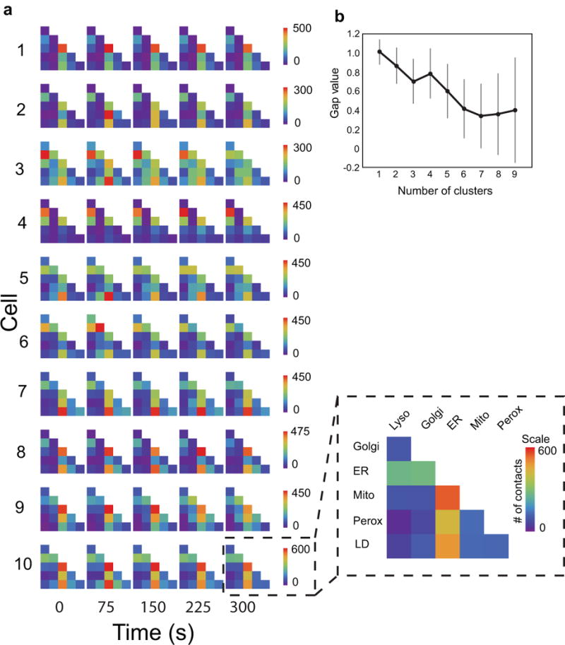
(a) The absolute numbers of organelle contacts in each cell at a single time point are displayed as graphical half matrices. Each row in the matrix represents the number of organelle contacts with each target organelle (columns), and is colour coded from 0 to maximum number of observed contacts in each cell. Each row of graphical matrices represents the organelle interactome in one cell and each column of graphical matrices represents the organelle interactome at a specific time point (0, 75, 150, 225 or 300 s). We performed an analysis of variance (ANOVA) in order to assess the variance in organelle-organelle contacts within cells over time. The results showed that the variance between cells is significantly larger than the variance within an individual cell across time (p<1×10^−37). (b) Cluster analysis of the organelle contact data for all ten cells. The gap statistic was calculated for 1–9 hypothetical clusters (see Statistics), and no meaningful differences were found to separate the organelle associations for the ten cells. This suggested there is a reproducible and scalable pattern of organelle contacts despite cell-to-cell differences in the absolute numbers of organelles. n = 100 simulations, error bars represent s.e.m.

Extended Data Figure 4. Validation of 6-colour labelling and organelle interaction measurements (confocal).

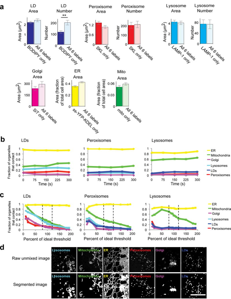
(a) To test the effect of co-expressing all six labels on organelle properties, we compared the number and/or area of organelles in cells singly transfected with one organelle marker or incubated with BODIPY, with cells labelled with all six organelle markers. For LDs, peroxisomes, and lysosomes, mean cross-sectional area and number were measured. For Golgi, total cross-sectional area/cell was measured. For ER and mitochondria, the fraction of cell area occupied by these organelles was measured. Only LD number showed a significant difference between singly- vs. multiply-labelled conditions. n = 20 cells for all 6 labelled cells, n = 20 cells (BODIPY only), n = 14 cells (SKL only), n = 21 cells (LAMP-1 only), n = 19 cells (SiT only), n = 18 cells (ER only), n = 20 cells (mito only). ** p < 0.01 (unpaired, two-tailed t-test). Bar heights represent mean values and error bars represent s.e.m. (b) Line graphs showing the fraction of LDs, peroxisomes or lysosomes contacting each of the other labelled organelles in one cell over time, measured discreetly at 0, 75, 150, 225 and 300 s. The fraction of total LDs, peroxisomes or lysosomes contacting each of the other organelles remained constant over the course of imaging, consistent with minimal perturbation and phototoxicity during the imaging period. (c) Line graphs showing the fraction of LDs, peroxisomes or lysosomes contacting each of the other labelled organelles in one cell (cell 1 in Extended Data Fig. 3a) after modulating the threshold value for all channels by a fixed percentage. Dashed lines represent a threshold modulated up or down by 20%. Ideal threshold = 100%. For all organelles except mitochondria, modulating the threshold up or down by up to 20% from the algorithmically determined optimal threshold value did not significantly alter the measured number of organelle contacts, suggesting that our organelle contact measurements are insensitive to small differences in threshold parameters. (d) Examples of segmentation based on algorithmically-determined, optimal intensity threshold values. Micrographs are representative of 10 cells captured. Scale bar, 10 μm.

Extended Data Figure 5. Effect of nocodazole on organelle contacts.

(a) Micrographs of a COS-7 cell labelled as in Fig. 1, except that instead of labelling Golgi, microtubules were labelled with mApple-MAP4-C10. i.-iii. Enlargements of the regions outlined in the left panel. iii.’ Region iii., without the ER displayed, for clarity. Lysosomes, mitochondria, the ER, peroxisomes, and LDs were all observed in close proximity to microtubules. Scale bars, 10 μm (left) and 2 μm (right). (b) The same cell as in (a), displaying only the microtubule channel, both before (left) and (after) treatment with 5 μM nocodazole for 1 h. Scale bar, 10 μm. Micrographs in (a) and (b) are representative of 20 cells captured. (c) Network diagrams of untreated and nocodazole-treated cells. Untreated network is the same as in Fig. 1d. After nocodazole treatment, the ER remains the central node in the network. (d) Comparison of object-based organelle contact analysis (bright) versus pixel-based organelle colocalization analysis (pastel). For the pixel-based analysis, a value of 1 indicates perfect co‐localization, while a value of 0 indicates the organelles are never co‐located. No statistical test was performed. (e) Comparison of the effect of nocodazole treatment on organelle contacts when images were analysed using either an object-based or pixel-based colocalization analysis scheme. Red lines connecting the median values indicate that the median number of contacts decreased after nocodazole treatment. Shown are all organelle contact pairs that showed a statistically significant change in contact frequency when cells were treated with nocodazole (unpaired, two-tailed t-test). (c-d) Object-based analysis data is the same as in Fig. 2a. n = 11 (nocodazole-treated) or n = 10 (untreated) cells from two experiments.

Extended Data Figure 6. Effect of starvation or excess fatty acids on organelle contacts.

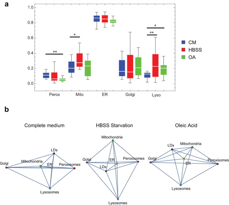
(a) Box whisker plots showing the fraction of LDs contacting each of the other labelled compartments in cells grown in complete medium (CM, blue), Hank’s balanced salt solution (HBSS, red), or complete medium supplemented with 300 μM oleic acid (OA, green) for 18 h. * 0.05 > p < 0.01, ** p < 0.01 (unpaired, two-tailed t-test). Error bars represent s.e.m. (b) Network diagrams showing the organelle interactome in cells treated as described in (a). (a-b) Complete medium data is the same as control data shown in Fig. 1d and Fig. 2a; n = 10 (complete medium), n = 15 (HBSS), or n = 14 (oleic acid) cells from two experiments.

Extended Data Figure 7. LLS spectral imaging and linear unmixing.

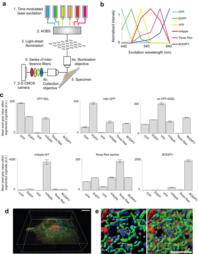
(a) Schematic of the hardware used for 6-colour light sheet microscopy. The specimen was excited using six lasers sequentially, by LLS illumination. Emitted light passed through a series of interference filters and was collected using a sCMOS camera. (b) Plot of the emission intensity of the indicated fluorophores as a function of excitation wavelength, in images of singly labelled cells acquired as described in (a). To identify fluorophores in the image data, we applied an excitation-side unmixing algorithm (see Image Acquisition and Unmixing). Our multispectral time-lapse LLS images consisted of upwards of 7 billion sets of 6 colour-channel pixels (547 × 640 pixels per plane × 140 planes per cell × 100 time points per cell × 10 cells). Because the solution to the unmixing operation at every pixel is independent of every other pixel, we distributed the unmixing operation over 32 cores of a computer workstation. (c) Plots of mean pixel intensity values for all 6 fluorophores in every pixel in singly labelled cells that were segmented as foreground. Cells were singly labelled with CFP-SKL, mito-EGFP, ss-YFP-KDEL, mApple-SiT, Texas Red dextran, or BODIPY 665/676. The error in LLS unmixing is higher than for confocal (see Extended Data Fig. 1f) as expected and is due partly to the fact that only six channels of spectral information were used to unmix the overlapping spectra. n = 149 pixels (CFP), n = 3,910 pixels (EGFP), n = 9,180 pixels (YFP), n = 1,549 pixels (mApple), n = 806 pixels (Texas Red Dextran), n = 3,248 pixels (BODIPY 667/676). Error bars represent s.e.m. (d) Tilted volume rendering of the same cell shown in Fig. 3a. Scale bar, 10 μm. (e) Zoomed, segmented images from the cell shown in (d). The left panel does not include the ER channel while the right panel does (transparent yellow). Scale bar, 5 μm. Micrographs in (d) and (e) are representative of 10 cells captured.

Extended Data Figure 8. Validation of organelle interaction measurements (LLS).

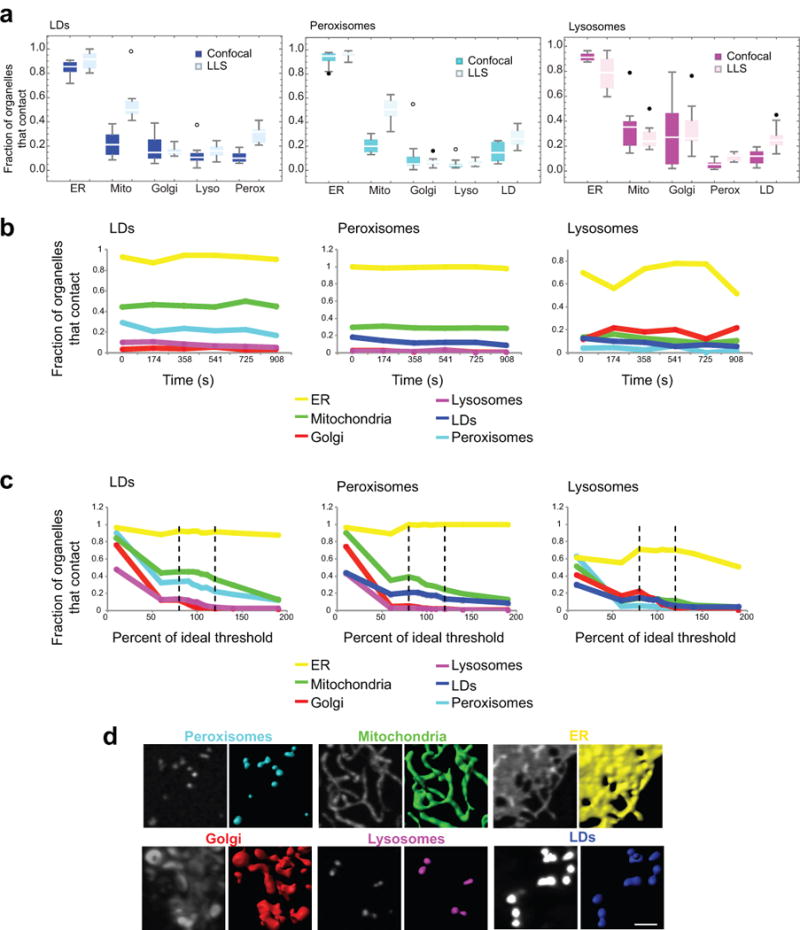
(a) Box whisker plots showing the median fraction of LDs, peroxisomes, or lysosomes making contact with each of the other labelled compartments in data obtained using confocal (bright) or LLS (pastel) microscopy. Confocal data is the same as in Fig. 2a. n = 10 cells (confocal), n = 10 cells (LLS). No statistical test was performed. The similarity in measurements from LLS and confocal images is likely because the globular organelles that we examined are smaller than the depth of focus of the confocal microscope, ensuring that all their inter-organelle interactions were detected even in the confocal images. (b) Line graphs showing the fraction of LDs, peroxisomes or lysosomes contacting each of the other labelled organelles in one cell measured over time at discreet points: 0, 174, 358, 541, 725 and 908 s. (c) Line graphs showing the fraction of LDs, peroxisomes or lysosomes contacting each of the other labelled organelles in one cell after modulating the threshold value for all channels by a fixed percentage. Dashed lines represent a threshold modulated by 20%. (d) Examples of segmentation performed using the ideal threshold (i.e., 100%) in (c). Scale bar, 2 μm. Micrographs are representative of 10 cells.

Extended Data Figure 9. Comparison of object- versus pixel-based analysis (LLS).

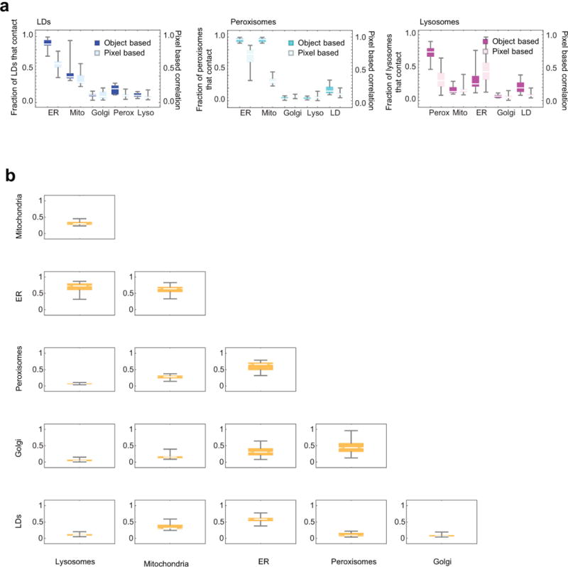
(a) Comparison of object-based organelle contact analysis (bright) versus pixel-based organelle colocalization analysis (pastel). Object-based analysis data is the same as LLS data in Extended Data Fig. 8a. For the pixel-based analysis, a value of 1 indicates perfect co‐localization, a value of 0 indicates the organelles are never co‐located. No statistical test was performed. (b) Half matrix showing pixel-based colocalization analysis for all the labelled organelle pairs, including those that were not included in the object-based analysis. Outliers were not identified. (a-b) n = 10 cells.

Extended Data Table 1. Measurements of organelle characteristics in COS-7 cells.

Values reported as mean +/− s.e.m. marked with * were measured in 3-D volume rendered images from the LLS spectral instrument, n=10 cells. Values reported as mean +/− s.e.m. marked with ^ˆ were measured in single z-plane confocal images of live cells, n=10 cells.

Organelle measurement	Value
Lipid droplets
Number per cell*	157 +/− 21
Mean volume*	0.41 +/− 0.05 μm3
Total volume per cell*	65 +/− 10 μm3
Maximum speed^	155.3+/−0.1 nm/s
Peroxisomes
Number per cell*	186+/−19
Volume*	0.27 +/− 0.02 μm3
Total volume per cell*	48 +/− 6 μm3
Maximum speed^	148.9 +/− 0.1 nm/s
Lysosomes
Number per cell*	89 +/− 10
Volume*	0.24 +/− 0.02 μm3
Total volume per cell	20 +/− 2 μm3
Maximum speed*	377.7+/− 0.1 nm/s
Golgi
Total volume per cell*	42 +/− 3 μm3
ER
Total volume per cell*	1538 +/− 178 μm3
Mitochondria
Total volume per cell*	179 +/− 20 μm3
ERMCSs
Number per cell^	550 +/− 90
Total area^	60 +/− 10 μm2
Whole Cell
Total volume per cell*	6074 +/− 464 μm2

Supplementary Material

vid1. Video 1: Point-scanning confocal, 6-colour time-lapse images.

COS-7 cells expressing fusion proteins targeted to the lysosomes (cyan), mitochondria (green), ER (yellow), peroxisomes (red), and Golgi (magenta), and labelled with BODIPY 665/676 to stain LDs (blue) were imaged as described in Fig. 1a. Images were acquired every 5 s, for a total of 60 frames (5 min). In frames 21–40, the ER channel (yellow) is omitted so that the other channels can be seen more clearly. Video plays at a rate of 6 frames per s. Scale bar, 10 μm.

vid2. Video 2: Time-lapse images of tracked LDs.

Videos of the tracked LDs (outlined in white) shown in Fig. 2b. Confocal images were acquired every 5 s, for a total of 60 frames (5 min). Video plays at a rate of 6 frames per s. Scale bar, 5 μm.

vid3. Video 3: Time-lapse images of a cell treated with nocodazole.

A COS-7 cell expressing fusion proteins targeted to the lysosomes (cyan), mitochondria (green), ER (yellow), peroxisomes (red), and Golgi (magenta), and labelled with BODIPY 665/676 to stain LDs (blue), was incubated on ice for 2 min and treated with 5 μM nocodazole for 1 h. After the nocodazole treatment, confocal images were acquired every 5 s, for a total of 60 frames (5 min). In frames 21–40, the ER channel (yellow) is omitted so that the other channels can be seen more clearly. Video plays at a rate of 6 frames per s. Scale bar, 10 μm.

vid4. Video 4: Lattice light sheet, 6-colour time-lapse images.

Volume rendering of COS-7 cells expressing fusion proteins targeted to the peroxisomes (cyan), mitochondria (green), ER (yellow), and Golgi (red), and labelled with Texas Red dextran (lysosomes, magenta) and BODIPY 665/676 (LDs, blue), imaged as described in Fig. 3a. Image stacks of 140 planes were acquired every 9.2 seconds, for a total of 100 frames (15.3 min). Video plays at a rate of 6 frames per s. Scale bar, 10 μm.

vid5. Video 5: Organelle dispersion through the cytoplasm over time.

Volume rendering of 6 organelles in a COS-7 cell. Voxels are colour-coded according to the time that they were last occupied by the organelle from blue to red.

vid6. Video 6: Montage of mitochondria-organelle contacts in time lapse, lattice light sheet images.

Volume rendering of mitochondria (magenta) in COS-7 cells expressing fusion proteins targeting 3 other organelles, and labelled with Texas Red dextran and BODIPY 665/676. Contacts between mitochondria and other organelles are coloured green. Image stacks of 140 planes were acquired every 9.2 seconds, for a total of 100 frames (15.3 min). Scale bar, 5 μm.

vid7. Video 7: Mitochondria-organelle contacts in time lapse, lattice light sheet images.

Volume rendering of mitochondria in COS-7 cells expressing fusion proteins targeting 3 other organelles, and labelled with Texas Red dextran and BODIPY 665/676. Contacts between mitochondria and other organelles are coloured yellow (ER), cyan (peroxisomes) red (Golgi), magenta (lysosomes) and blue (LDs). Image stacks of 140 planes were acquired every 9.2 seconds, for a total of 100 frames (15.3 min). Scale bar, 10 μm.

vid8. Video 8: Mitochondria-ER metaorganelle contacts with other organelles.

Volume rendering of mitochondria-ER contacts in COS-7 cells expressing fusion proteins targeting 2 other organelles, and labelled with Texas Red dextran and BODIPY 665/676. Contacts between mitochondria-ER metaorganelle and other organelles are coloured cyan (peroxisomes) red (Golgi), magenta (lysosomes) and blue (LDs). Image stacks of 140 planes were acquired every 9.2 seconds, for a total of 100 frames (15.3 min). Scale bar, 10 μm.

References

- 1.Barbosa AD, Savage DB, Siniossoglou S. Lipid droplet–organelle interactions: emerging roles in lipid metabolism. Curr Opin Cell Biol. 2015;35:91–97. doi: 10.1016/j.ceb.2015.04.017. [DOI] [PubMed] [Google Scholar]
- 2.Shai N, Schuldiner M, Zalckvar E. No peroxisome is an island - Peroxisome contact sites. Biochim Biophys Acta. 2015 doi: 10.1016/j.bbamcr.2015.09.016. [DOI] [PMC free article] [PubMed] [Google Scholar]
- 3.Settembre C, Fraldi A, Medina DL, Ballabio A. Signals from the lysosome: a control centre for cellular clearance and energy metabolism. Nat Rev Mol Cell Biol. 2013;14:283–296. doi: 10.1038/nrm3565. [DOI] [PMC free article] [PubMed] [Google Scholar]
- 4.Tatsuta T, Scharwey M, Langer T. Mitochondrial lipid trafficking. Trends Cell Biol. 2014;24:44–52. doi: 10.1016/j.tcb.2013.07.011. [DOI] [PubMed] [Google Scholar]
- 5.Phillips MJ, Voeltz GK. Structure and function of ER membrane contact sites with other organelles. Nat Rev Mol Cell Biol. 2016;17:69–82. doi: 10.1038/nrm.2015.8. [DOI] [PMC free article] [PubMed] [Google Scholar]
- 6.Rowland AA, Chitwood PJ, Phillips MJ, Voeltz GK. ER contact sites define the position and timing of endosome fission. Cell. 2014;159:1027–1041. doi: 10.1016/j.cell.2014.10.023. [DOI] [PMC free article] [PubMed] [Google Scholar]
- 7.Friedman JR, et al. ER tubules mark sites of mitochondrial division. Science. 2011;334:358–362. doi: 10.1126/science.1207385. [DOI] [PMC free article] [PubMed] [Google Scholar]
- 8.Wilfling F, et al. Arf1/COPI machinery acts directly on lipid droplets and enables their connection to the ER for protein targeting. eLife. 2014;3:e01607. doi: 10.7554/eLife.01607. [DOI] [PMC free article] [PubMed] [Google Scholar]
- 9.Neher R, Neher E. Optimizing imaging parameters for the separation of multiple labels in a fluorescence image. J Microsc. 2004;213:46–62. doi: 10.1111/j.1365-2818.2004.01262.x. [DOI] [PubMed] [Google Scholar]
- 10.Chen BC, et al. Lattice light-sheet microscopy: Imaging molecules to embryos at high spatiotemporal resolution. Science. 2014;346:1257998. doi: 10.1126/science.1257998. [DOI] [PMC free article] [PubMed] [Google Scholar]
- 11.Herms A, et al. AMPK activation promotes lipid droplet dispersion on detyrosinated microtubules to increase mitochondrial fatty acid oxidation. Nat Commun. 2015;6 doi: 10.1038/ncomms8176. [DOI] [PMC free article] [PubMed] [Google Scholar]
- 12.Friedman JR, Webster BM, Mastronarde DN, Verhey KJ, Voeltz GK. ER sliding dynamics and ER–mitochondrial contacts occur on acetylated microtubules. J Cell Biol. 2010;190:363–375. doi: 10.1083/jcb.200911024. [DOI] [PMC free article] [PubMed] [Google Scholar]
- 13.de Forges H, Bouissou A, Perez F. Interplay between microtubule dynamics and intracellular organization. Int J Biochem Cell Biol. 2012;44:266–274. doi: 10.1016/j.biocel.2011.11.009. [DOI] [PubMed] [Google Scholar]
- 14.Friedman JR, Dibenedetto JR, West M, Rowland AA, Voeltz GK. Endoplasmic reticulum-endosome contact increases as endosomes traffic and mature. Mol Biol Cell. 2013;24:1030–1040. doi: 10.1091/mbc.E12-10-0733. [DOI] [PMC free article] [PubMed] [Google Scholar]
- 15.Wait E, et al. Visualization and correction of automated segmentation, tracking and lineaging from 5-D stem cell image sequences. BMC Bioinformatics. 2014;15:1–14. doi: 10.1186/1471-2105-15-328. [DOI] [PMC free article] [PubMed] [Google Scholar]
- 16.Rambold AS, Cohen S, Lippincott-Schwartz J. Fatty Acid Trafficking in Starved Cells: Regulation by Lipid Droplet Lipolysis, Autophagy, and Mitochondrial Fusion Dynamics. Dev Cell. 2015;32:678–692. doi: 10.1016/j.devcel.2015.01.029. [DOI] [PMC free article] [PubMed] [Google Scholar]
- 17.Singh R, et al. Autophagy regulates lipid metabolism. Nature. 2009;458:1131–1135. doi: 10.1038/nature07976. [DOI] [PMC free article] [PubMed] [Google Scholar]
- 18.Ikonen E. Cellular cholesterol trafficking and compartmentalization. Nat Rev Mol Cell Biol. 2008;9:125–138. doi: 10.1038/nrm2336. [DOI] [PubMed] [Google Scholar]
- 19.Eisenberg-Bord M, Shai N, Schuldiner M, Bohnert M. A Tether Is a Tether Is a Tether: Tethering at Membrane Contact Sites. Dev Cell. 2016;39:395–409. doi: 10.1016/j.devcel.2016.10.022. [DOI] [PubMed] [Google Scholar]
- 20.Patterson GH. A Photoactivatable GFP for Selective Photolabeling of Proteins and Cells. Science. 2002;297:1873–1877. doi: 10.1126/science.1074952. [DOI] [PubMed] [Google Scholar]
- 21.Snapp EL, Sharma A, Lippincott-Schwartz J, Hegde RS. Monitoring chaperone engagement of substrates in the endoplasmic reticulum of live cells. Proc Natl Acad Sci. 2006;103:6536–6541. doi: 10.1073/pnas.0510657103. [DOI] [PMC free article] [PubMed] [Google Scholar]
- 22.Kim PK, Mullen RT, Schumann U, Lippincott-Schwartz J. The origin and maintenance of mammalian peroxisomes involves a de novo PEX16-dependent pathway from the ER. J Cell Biol. 2006;173:521–532. doi: 10.1083/jcb.200601036. [DOI] [PMC free article] [PubMed] [Google Scholar]
- 23.Jahr W, Schmid B, Schmied C, Fahrbach FO, Huisken J. Hyperspectral light sheet microscopy. Nat Commun. 2015;6:7990. doi: 10.1038/ncomms8990. [DOI] [PMC free article] [PubMed] [Google Scholar]
- 24.Otsu N. A Threshold Selection Method from Gray-Level Histograms. IEEE Trans Syst Man Cybern. 1979;9:62–66. [Google Scholar]
- 25.Jaqaman K, et al. Robust single-particle tracking in live-cell time-lapse sequences. Nat Methods. 2008;5:695–702. doi: 10.1038/nmeth.1237. [DOI] [PMC free article] [PubMed] [Google Scholar]
- 26.Gatta AT, Levine TP. Piecing Together the Patchwork of Contact Sites. Trends Cell Biol. 2016 doi: 10.1016/j.tcb.2016.08.010. [DOI] [PubMed] [Google Scholar]
- 27.Gonzales R, Woods R, Eddins S. Digital Image Processing Using MATLAB. 2nd. Gatesmark Publishing; 2009. [Google Scholar]
- 28.Winter M, Mankowski W, Wait E, Temple S, Cohen AR. LEVER: software tools for segmentation, tracking and lineaging of proliferating cells. Bioinformatics. 2016 doi: 10.1093/bioinformatics/btw406. btw406. [DOI] [PMC free article] [PubMed] [Google Scholar]
- 29.Cohen AR, Bjornsson C, Temple S, Banker G, Roysam B. Automatic summarization of changes in biological image sequences using algorithmic information theory. IEEE Trans Pattern Anal Mach Intell. 2009;31 doi: 10.1109/TPAMI.2008.162. [DOI] [PubMed] [Google Scholar]
- 30.Tibshirani R, Walther G, Hastie T. Estimating the number of clusters in a data set via the gap statistic. J R Stat Soc Ser B Stat Methodol. 2001;63:411–423. [Google Scholar]
Extended Data References
- 31.Garini Y, Young IT, McNamara G. Spectral imaging: Principles and applications. Cytometry A. 2006;69A:735–747. doi: 10.1002/cyto.a.20311. [DOI] [PubMed] [Google Scholar]
- 32.Valm AM, et al. Systems-level analysis of microbial community organization through combinatorial labeling and spectral imaging. Proc Natl Acad Sci U S A. 2011;108:4152–4157. doi: 10.1073/pnas.1101134108. [DOI] [PMC free article] [PubMed] [Google Scholar]
- 33.Valm AM, Oldenbourg R, Borisy GG. Multiplexed Spectral Imaging of 120 Different Fluorescent Labels. PloS One. 2016;11:e0158495. doi: 10.1371/journal.pone.0158495. [DOI] [PMC free article] [PubMed] [Google Scholar]
- 34.Tsuriel S, Gudes S, Draft RW, Binshtok AM, Lichtman JW. Multispectral labeling technique to map many neighboring axonal projections in the same tissue. Nat Methods. 2015;12:547–552. doi: 10.1038/nmeth.3367. [DOI] [PubMed] [Google Scholar]
- 35.Shaner NC, Steinbach PA, Tsien RY. A guide to choosing fluorescent proteins. Nat Methods. 2005;2:905–909. doi: 10.1038/nmeth819. [DOI] [PubMed] [Google Scholar]
- 36.Rodriguez EA, et al. A far-red fluorescent protein evolved from a cyanobacterial phycobiliprotein. Nat Methods. 2016;13:763–769. doi: 10.1038/nmeth.3935. [DOI] [PMC free article] [PubMed] [Google Scholar]
- 37.The molecular probes handbook: a guide to fluorescent probes and labeling technologies. Life Technologies; 2010. [Google Scholar]
- 38.Dickinson ME, Bearman G, Tille S, Lansford R, Fraser SE. Multi-spectral imaging and linear unmixing add a whole new dimension to laser scanning fluorescence microscopy. BioTechniques. 2001;311278:1272, 1274–1276. doi: 10.2144/01316bt01. [DOI] [PubMed] [Google Scholar]
- 39.Schneider CA, Rasband WS, Eliceiri KW. NIH Image to ImageJ: 25 years of image analysis. Nat Methods. 2012;9:671–675. doi: 10.1038/nmeth.2089. [DOI] [PMC free article] [PubMed] [Google Scholar]
Associated Data
This section collects any data citations, data availability statements, or supplementary materials included in this article.
Supplementary Materials