Does Machine Learning Automate Moral Hazard and Error?

Machine learning is poised to transform health care. For example, to diagnose certain diabetic complications, ophthalmologists must visualize patients’ retinae, looking for subtle signs of damage. A Google team built a deep learning algorithm that could look at digitized retinal photographs and diagnose as accurately, if not more, than physicians (Gulshan et al. (2016)).

These efforts, though, are expanding in scope, from automating routine tasks to aiding in complex decisions. Tailored diagnostics help doctors decide whom to test and treat. Algorithms predict adverse outcomes (say stroke or heart disease) for early warning system that target resources and attention to high-risk patients.

These health policy applications raise their own econometric concerns. One is well understood—the conflation of causation and prediction. We suggest another important, yet under-appreciated, challenge: mismeasurement. Machine learning algorithms excel at predicting outcomes y based on inputs x. In automation tasks, measuring y, e.g. majority opinion of ophthalmologists, is straightforward. In health policy applications, we rely on electronic health records or claims data to measure y and x. The very construction of these data induces large and systematic mismeasurement. These in turn can bias algorithmic predictions; in some cases, these biases can automate policies that magnify existing clinical errors and moral hazard.

I. Example Application

Patients in the emergency department (ED) can be difficult to diagnose. Subtle symptoms can often overlap between diseases of differing severity: nausea could reflect heart attack, or acid reflux. Take the case of patients who are either having a stroke, or are at high risk of impending stroke in the days after ED visits. These patients can be hard to distinguish from more benign presentations. Yet if they could be identified, one could target more effective interventions in the ED, or arrange for close follow-up and expedited additional testing (e.g., to identify treatable causes of potential stroke) if they are sent home.

This seems like a perfect example of a ‘prediction problem’ (Kleinberg et al. (2015)). This decision does not require a causally valid estimate of a coefficient β̂_x, such as how a particular treatment affects stroke risk. Instead, we require an accurate prediction ŷ of stroke risk y in order to allocate interventions to highest risk patients. Moreover, the richness of electronic health records (EHRs) give us many variables x with which to make these predictions.

A. Empirical Results

To illustrate this, we use data from a large academic hospital and its ED to predict short-term stroke risk, focusing on a diagnosis of stroke in the week of the ED visit. As predictors, we use demographic data as well as any prior diagnoses present in the EHR system over the year before the ED visit, grouped into clinically-relevant categories. To illustrate our point simply, we use a logistic regression; surely more complex predictors would find even more structure than we present.¹

Table 1 presents the top predictors of future stroke in terms of coefficient magnitude. Somewhat intuitively, prior stroke has the strongest association with future stroke. The next five largest predictors of stroke are also shown. Like prior stroke, history of cardiovascular disease also makes sense as a known risk factor for stroke. The other four predictors—accidental injury, benign breast lump, colonoscopy, and sinusitis—are somewhat more mysterious. Have we discovered novel biomedical risk factors for stroke?

Table 1.

Predicting and Mispredicting

	Stroke	30 Day Mortality
Prior Stroke	.302*** (.012)	.041*** (.014)
Prior Accidental Injury	.285** (.095)	.007 (.101)
Abnormal Breast Finding	.224* (.092)	.162 (.110)
Cardiovascular Disease History	.218*** (.029)	−.017 (.034)
Colon Cancer Screening	.242 (.178)	−.475** (.222)
Acute Sinusitis	.220 (.155)	.056 (.166)

Notes: Logistic regression on demographics and prior diagnoses in EHR data. Sample: 177,825 ED visits in 2010-2 to a large academic hospital.

B. Measurement

To understand what might be happening, we must understand the measurement process underlying these data. We have spoken as if we are predicting “stroke.” Yet our measures are several layers removed from the biological signature of blood flow restriction to brain cells. Instead we see the presence of a billing code or a note recorded by a doctor. Moreover, unless the stroke is discovered during the ED visit, the patient must have either decided to return, or mentioned new symptoms to her doctors during hospital admission that provoked new testing. In other words, measured stroke is (at least) the compound of: having stroke-like symptoms, deciding to seek medical care, and being tested and diagnosed by a doctor.

Medical data are as much behavioral as biological; whether a person decides to seek care can be as pivotal as actual stroke in determining whether they are diagnosed with stroke. Many decisions and judgments intervene in the assignment of a diagnosis code—or indeed, any piece of medical data, including obtaining and interpreting test results, admission and re-admission of a patient to the hospital, etc.

Viewed in this light, the findings in Table 1 are intuitive. We are just as much predicting heavy utilization (the propensity of people to seek care) as we are biological stroke. For example, evaluation for minor injury implies that the patient came into her doctor’s clinic or the ED for minor injuries; a recorded abnormal breast finding indicates that she noticed an irregularity, worried about it enough to schedule a visit, and came in to be checked out. Variables which proxy for heavy utilization could in fact appear to predict any medical condition, including stroke.

This can be seen by looking at a variable far less prone to mis-measurement: mortality. Column (2) shows coefficients for a similar regression in which mortality (ascertained from Social Security Administration records) is substituted for stroke as the dependent variable. All coefficients have decreased in magnitude. We can see that prior stroke remains associated with mortality, but the two significant predictors of stroke (injury and breast lump) no longer predict mortality; screening for colon cancer has switched signs and become a strong negative predictor of mortality. All in all, we can see that the variables that were so effective at predicting a y measured through the lens of human decision-making no longer perform so well in predicting a y measured with less error.

II. Measurement error in medical prediction problems

A simple framework can help understand how mismeasurement might bias prediction. We can write this as the difference between y_i, e.g., measured stroke from medical records, and actual stroke, $y_i^{\ast }$:

$$y_i=y_i^{\ast }+{\mathrm{\Delta }}_i$$

In a causal inference task, we have some intuition about how mis-measurement can be problematic: if Δ_i is correlated with a variable, its coefficient will be biased. How will it matter for prediction tasks?

A good predictor will produce predictions that are close to expected values:

$$\widehat{y_i}\approx E[y_i\mid x_i]=E[y_i^{\ast }\mid x_i]+E[{\mathrm{\Delta }}_i\mid x_i]$$

Since we care about the prediction as a whole, in principle we are no longer concerned that Δ_i is correlated with specific x_i variables but with any predictor. Two scenarios are possible here. The best case is that the error Δ_i is noise uncorrelated with x_i.

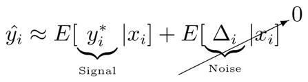The resulting prediction will be purely fitted to the predictable part of underlying risk, rather than the error. Here, prediction will effectively be a ‘denoised’ version of the raw y_i drawn from medical records.

A less optimistic scenario arises when both error and actual risk are predictable:

$$\widehat{y_i}\approx \underset{\text{Signal}}{\underbrace{E[y_i^{\ast }\mid x_i]}}+\underset{\text{Predictable}\text{error}}{\underbrace{\stackrel{\ne 0}{\overbrace{E[{\mathrm{\Delta }}_i\mid x_i]}}}}$$

By writing $\widehat{y_i^{\ast }}=E[y_i^{\ast }\mid x_i]$ and Δ̂_i E[Δ_i|x_i], prediction variability can be decomposed in to the the predictable variance of the signal and the noise:

$$\mathit{var}({\widehat{y}}_i)=\mathit{var}(\widehat{y_i^{\ast }})+\mathit{var}({\widehat{\mathrm{\Delta }}}_i)+2\mathit{cov}(\widehat{y_i^{\ast }},{\widehat{\mathrm{\Delta }}}_i)$$

How much our decisions are based on predicted risk, ŷ, versus how much they are based on mismeasurement depends on the relative predictability of $y_i^{\ast }$ and Δ_i.

This simple framework helps makes sense of our empirical example. In this case:

$$\begin{array}{lll}\underset{\text{Measured}\text{Stroke}}{\underbrace{y_i}}& =& \underset{\text{Stroke}}{\underbrace{y_i^{\ast }}}+\underset{\text{Heavy}\text{Utilizer}}{\underbrace{{\mathrm{\Delta }}_i}}\\ \underset{\text{Measured}\text{Injury}}{\underbrace{x_i}}& =& \underset{\text{Injury}}{\underbrace{x_i^{\ast }}}+\underset{\text{Heavy}\text{Utilizer}}{\underbrace{{\mathrm{\Delta }}_i^x}}\end{array}$$

Measured injury predicts measured stroke because both are proxies for heavy utilization patients. Our (measured) stroke predictor is actually a combination of a stroke predictor and a utilization predictor.

In fact, given the nature of the data, it is entire plausible that utilization, Δ_i, is more predictable than $y_i^{\ast }$, true stroke outcome. After all most of our predictors are highly dependent on patients tendency to utilize. In this sense, an early warning system based on predicted stroke risk might magnify moral hazard—by diverting resources even further to patients most likely to seek out care.

A. Consequences for decisions

In most machine learning applications, ŷ feeds into some decision. In the stroke example above, the decision is whether or not to allocate high-cost diagnostic or therapeutic technology to a patient with a given level of predicted risk.

Predictability of error alone does not imply a problem for decision-making. For example, the misprediction may not distort the the rank ordering of individuals in terms of $\widehat{y_i}$. In these cases any decision that allocates according to rank, such as D_i = 1 if $\widehat{y_i}>(c/b)$ (based on costs and benefits of D) will not be affected. The decision can simply be scaled back to a new threshold $\widehat{y_i}>(c/b)+k$, where k is an approximation of E[Δ_i|x_i]. As an example, if the only error in y_i was that moral hazard led doctors to over-diagnose stroke, but $\widehat{y_i}$ still consistently ranked patients by true risk, we could simply scale back decisions (e.g., allocate D to the top 5% instead of the top 10% as the original prediction would have suggested).

In many cases, however, mismeasurement distorts rank ordering as well. The stroke predictor above did not simply rank according to true stroke risk: patients could have higher predicted “stroke risk” simply by being heavy utilizers. In these cases, predictors will create decision and allocation biases. The severity of these biases—and whether they lead to worse outcomes—depends on how predictable mismeasurement is, relative to the underlying outcome. As we have seen, in health data, mismeasurement is plausibly even more predictable than true risk. An important corollary is that simply quantifying how well algorithms predict measured y is not enough to gauge its quality: we might prefer a worse-looking predictor that tracks true risk and does not fit to mismeasurement.

B. How widespread are these problems?

Measurement error is often ignored in the machine learning literature because it is largely unimportant in traditional applications. The image algorithms that underlie the self-driving car, for example, are trained on data where it is easy to objectively label the presence of road boundaries, pedestrians, trees, and other obstacles. In the large image datasets on which vision algorithms are trained, the judgment of human observers who label images defines the truth that algorithm designers seek to predict.

In health data, on the other hand, mismeasurement is the rule, and the example of stroke prediction is hardly the exception. We identify three major categories of mismeasurement.

First, measurement is subjective. A diagnosis is not an objective assessment, but rather an opinion that has been assigned and billed, often for the purpose of justifying further testing or treatment. Even symptoms are not unfiltered reports from patients, but rather those symptoms elicited in the course of an interview, redacted, and set down in a note.

Second it is selective. Diagnostic test results reflect the decision to test. Patients ‘set the agenda’ and select which complaints to focus on during a visit.

Finally, it is event-based. We only record data when there is some precipitating medical event, such as clinic visit or hospitalization.² We have seen how patient decisions play a major role here.

These measurement issues, in turn, can bias machine learning applications. First, as we saw above, they can further concentrate health spending in high utilizers. Many early warning systems are built on predictors not unlike our simple stroke predictor. These efforts to target testing, screening or simply extra attention may simply end up targeting the patients who already tend to seek out care at high levels.

Second, automated diagnoses could reinforce physicians’ judgmental biases (Blumenthal-Barby and Krieger (2015)). For example, if psychologically salient or available diseases are over-diagnosed, algorithms trained on these diagnoses might simply replicate them (Mamede et al. (2010)). These biases might also reinforce disadvantage. Physicians are 40% less likely to refer female or black patients with chest pain for catheterization (Schulman et al. (1999)). Minorities receive less aggressive cancer treatment (Bach et al. (1999)). Algorithms that mine EHR data to automate diagnoses or make personalized cancer treatment recommendations (e.g., IBM Watson’s) could perpetuate these biases.

In summary, measurement error can feed through prediction algorithms. The biases inherent in human decisions that generate the data could be automated or even magnified. Done naively, algorithmic prediction could then magnify or perpetuate some of policy problems we see in the health system, rather than fix them.

III. Solutions

Ultimately, just as for causal inference in observational data, we are unlikely to find a one size fits all solution to measurement problems in prediction tasks. But we can start to think about several categories of ways to mitigate or solve them.

One avenue is better measurement: in many cases, at some cost, better measure y. Because these measures are time consuming and expensive, it limits sample size to the point where machine learning is often impractical. One solution would be to use these on a small sample for validation. They could be taken after predictions are made using a potentially mismeasured y.³ These studies could even be combined with randomized trials of interventions, which would allow for both prediction of y^* and estimation of treatment effect by ŷ.

The ideal solution could be to hold machine learning tools to the same stnadard as any other new diagnostic technology in medicine, such as a new laboratory or imaging test. Their predictions ought to be compared to gold standard measures and rely on long-term, high-quality follow-up data for validation.

IV. Conclusion

Machine learning relies on the availability of large, high-quality datasets (Halevy et al. (2009)). Health policy is a particularly attractive area exactly because large data are increasingly becoming available. Yet if we do not take the measurement process generating those data seriously, predictive algorithms risk doing less good than they otherwise might; in some cases, they could possibly even do harm.

References

- Bach Peter B, Cramer Laura D, Warren Joan L, Begg Colin B. Racial differences in the treatment of early-stage lung cancer. New England Journal of Medicine. 1999;341(16):1198–1205. doi: 10.1056/NEJM199910143411606. [DOI] [PubMed] [Google Scholar]
- Blumenthal-Barby JS, Krieger Heather. Cognitive biases and heuristics in medical decision making: a critical review using a systematic search strategy. 2015;35(4):539–557. doi: 10.1177/0272989X14547740. [DOI] [PubMed] [Google Scholar]
- Gulshan Varun, Peng Lily, Coram Marc, et al. Development and validation of a deep learning algorithm for detection of diabetic retinopathy in retinal fundus photographs. JAMA. 2016;316(22):2402–2410. doi: 10.1001/jama.2016.17216. [DOI] [PubMed] [Google Scholar]
- Halevy Alon, Norvig Peter, Pereira Fernando. The unreasonable effectiveness of data. IEEE Intelligent Systems. 2009;24(2):8–12. [Google Scholar]
- Kleinberg Jon, Ludwig Jens, Mullainathan Sendhil, Obermeyer Ziad. Prediction policy problems. The American Economic Review. 2015;105(5):491–495. doi: 10.1257/aer.p20151023. [DOI] [PMC free article] [PubMed] [Google Scholar]
- Mamede Slvia, van Gog Tamara, van den Berge Kees, et al. Effect of Availability Bias and Reflective Reasoning on Diagnostic Accuracy Among Internal Medicine Residents. 2010;304(11):1198–1203. doi: 10.1001/jama.2010.1276. [DOI] [PubMed] [Google Scholar]
- Schulman Kevin A, Berlin Jesse A, Harless William, et al. The effect of race and sex on physicians’ recommendations for cardiac catheterization. New England Journal of Medicine. 1999;340(8):618–626. doi: 10.1056/NEJM199902253400806. [DOI] [PubMed] [Google Scholar]