

Abstract
Classifying brain white matter fibers into bundles is of growing interest in neuroscience. Quantification of diffusion characteristics inside a fiber bundle provides new insights for disease evolutions, therapy effects, and surgical interventions. In this paper, we present a novel method for segmenting fiber bundles using Spherical Harmonic Coefficients (SHC) which describe diffusion signal obtained from High Angular Resolution Diffusion Imaging (HARDI) protocols. Based on SHC, we define a similarity measure and use it as a speed function term in level set framework. We show advantages of the proposed measure over similarity measures based on Diffusion Tensor Imaging (DTI) indices. Without any assumptions about diffusion model, we deal with diffusion signal instead of orientation distribution function (ODF) calculated using complicated mathematics, inaccurate simplifications, and time-consuming implementation. By applying the proposed algorithm on synthetic data, its superior accuracy and robustness in low SNR conditions are shown. Application of the proposed method on real HARDI MRI data also illustrates its superior performance, especially in heterogeneous diffusion areas with low traditional diffusion anisotropies.
Keywords: Fiber bundle Segmentation, Spherical Harmonic Coefficients, Level Set, Diffusion MRI
I. Introduction
Diffusion magnetic resonance imaging (MRI) is a non-invasive tool to investigate white matter structure within the brain. It quantifies macroscopic diffusion of water molecules which is barred or hindered by microscopic structures. Basser et al [1, 2] assume a three dimensional Gaussian profile for the diffusion of water molecules and model its behavior by a symmetric positive semi-definite matrix (tensor). The tensor model can describe Gaussian diffusion behavior which is valid for free diffusion or isotropic restricted diffusion in all directions or anisotropic diffusion of just one major white matter fiber population. However, it fails to model higher order anisotropies in heterogeneous areas where more than one fiber population exist. For this reason, a clinically feasible image acquisition scheme with a large number of diffusion synthesizer gradients is introduced and named High Angular Resolution Diffusion Imaging (HARDI). Model-based analysis methods such as Multi-Tensor fitting [4], Spherical Deconvolution [5,6], non-linear Spherical Deconvolution [7] or PASMRI [8] and model-free analysis methods like q-ball [9] are proposed to analyze the HARDI data in order to obtain Orientation Distribution Function (ODF) from which main diffusion directions are extracted. However, using ODF instead of pure diffusion signal needs simplifications and approximations that make ODF calculation almost impractical as a preprocessing step.
It is straightforward to visualize tensor and diffusion signal or profile within the brain white matter. However, reconstruction of virtual fiber paths is preferred as it presents virtual anatomical connectivity within the brain and gives superior understanding of the underlying diffusion profile in voxels. To this end, one can track individual fibers (tractography) and extract curvilinear trajectories in three-dimensional (3D) space using the Diffusion Tensor Imaging (DTI) or the HARDI data. Tractography provides a qualitative understanding of the neural connectivity which is often hard to quantify. Quantitative measures are crucial for diagnosing neurological diseases and planning surgical procedures. An approach that provides quantitative measures of connectivity and is typically more robust than tractography, is segmentation of volumetric regions containing similar local diffusivity characteristics or similar fibers in shape and length as distinct objects named fiber bundles. A single fiber is defined as a region containing spatially compact and coherent axons. Similarly, a fiber bundle is defined as a region that contains spatially compact and coherent fibers in tabular structures like cortico-spinal or in planar structures like corpus-callosum. Extracting such bundles makes it possible to quantify the diffusion characteristics inside them and opens new insights for monitoring disease evolution of neurologic disorders like Multiple Sclerosis, Epilepsy, Stroke, Alzheimer, and Parkinson as well as evaluating therapy effects and mapping important brain connectivities that must be preserved during surgical interventions.
The task of classifying the brain white matter fibers can be performed by the following methods: clustering of the fibers resulted from tractography into bundles [10,11] or segmenting bundles via front propagation based on local properties of diffusion tensor, diffusion signal or ODF [12–19]. Since clustering methods rely on the tractography results, they will not work properly if the tractography step is not performed well. This is particularly the case for streamline types in critical situations like kissing, branching, merging and crossing status. The front propagation approach, without passing through the tractography step, is a more powerful tool, especially in the above conditions. Some of the front propagation methods, however, concentrate on the scalar quantities like anisotropy maps derived from the tensor data which do not reflect the complete tensor information [12]. Other methods, on the other hand, benefit from the whole information contained in the diffusion tensor imaging data [13–16]. They typically extract a similarity measure between the successive tensors and then insert these measures into a region-based segmentation framework like level set [17]. When segmenting white matter regions in DTI, the similarity measure must emphasize on anisotropic regions. The tensor model fits a planar or spherical tensor shape to the multimodal diffusion profile in heterogeneous areas with more than one major fiber population. Therefore, any similarity measure defined between the neighboring tensors prevents the front from propagating from a voxel with one major fiber population (with prolate tensor fit) into the next voxel that includes the same fiber population plus other fiber populations in different orientations (with oblate or spherical tensor fit). The reason is that any tensor-based similarity between a prolate tensor and an oblate or spherical one is negligible.
In a different study, a Position-Orientation Space (POS) is introduced by combining the geometric space with the spherical ODF space from the HARDI data. Here, two crossing fiber populations with different orientations in the spatial domain are resolved by applying a front propagation method in the level set framework in a 5-dimensional space [18]. In [19], fiber bundle segmentation is performed in POS based on Markov Random Fields (MRF). Assuming spatial relationships modeled by the MRF, this method estimates a hidden random field of fiber bundles from the observed ODF profiles using a Maximum A Posteriori (MAP) formulation and Iterative Conditional Modes (ICM) implementation. However, dimensional reinforcement of the problem causes disadvantages like increasing the computational cost. Compared to the statistical approach, the level set method takes into account several properties when formulating the segmentation problem. While most of the tractography methods demand a regularization of the data field, the level set method, in contrast, smoothes the propagating front automatically. It leads to a regularized segmentation process with sub-voxel precision, which is hard to achieve by other segmentation methods. In [20], a region-based statistical surface evolution on the image of ODF’s is applied to find coherent white matter fiber bundles. This method is claimed to be capable of propagating through regions of fiber crossings, where the state-of-the-art diffusion tensor imaging segmentation methods fail to do so.
In previous works, mostly diffusion probability density function or the ODF are derived from the diffusion signal by time-consuming transformations. The results are then used in the segmentation process. The downsides are that not only accurate ODF derivation is not feasible, but also the crossing fiber bundles are less resolvable in the domain of ODF than the diffusion signal.
Here, we present a novel segmentation framework to obtain the fiber bundles using Spherical Harmonic Coefficients (SHC) that describe diffusion signals obtained from the HARDI protocols. Expanding a spherical function by Spherical Harmonic (SH) bases, the SHC’s are obtained. They are descriptor features of the function on the sphere [21, 24]. The SHC’s are used to define a new similarity measure that detects subtle differences of the diffusion signals in the neighboring voxels by using almost all information contained in the diffusion data. To segment the fiber bundles, we assume that the neighboring voxels within the same bundle have similar diffusion properties. We utilize the level set framework and define its speed function term based on the proposed similarity measure. It is shown that our method has advantages over the methods that use similarity measures based on the DTI. This is done by proper propagation of the front within the fiber crossing areas. Without any assumptions about the diffusivity profile or the model, the proposed method deals with the diffusion signal instead of the ODF commonly used in the literature. Experimental results demonstrate the capability of the proposed method in detecting artificial crossing bundle patterns, even in low SNR conditions. By applying the proposed method on the real HARDI MRI data, we segment some of the major fiber bundles like Corpus Callosum (CC), Cingulum (Cg), and Cortico-Spinal (CS) tracts. The superiority of the proposed method to resolve the crossing fiber bundles and to find the whole tracts is illustrated by comparing our results with those of the previous methods.
In contrast to the work of Descoteaux and Deriche [20] that maximizes the a-posterior probability based on the observed ODF’s and assumes Gaussian distributions in different partitions of the Q-ball images, our proposed method uses the similarity between the SH of the ODF’s directly in the speed term of the level set without any assumptions. Moreover, it uses the SH coefficients with the order of 8 which is consistent with the ODF’s with up to four major peaks.
In the next section, the theory underlying the spherical harmonic coefficients is described. Then, the level set numerical method is briefly reviewed. In the third section, spherical harmonic characteristics are explained and the results of the proposed method on the simulated crossing pattern and real HARDI data are presented and discussed. Finally, in the fourth section, the proposed method and its advantages are summarized.
II. Methods
a) Spherical Harmonic Coefficients
The expansion of a function on a sphere using spherical harmonics is equivalent to the generalization of Fourier representation to the spherical coordinates [23, 24]. By expanding the diffusion signals of the HARDI data using these basis harmonics and calculating the harmonic coefficients, a linear method for calculating ODF has been proposed [21, 22].
The spherical harmonics, represented by (l is the order and m is the phase factor), are the bases for the complex functions on the unit sphere. They are defined by:
| (1) |
where θ ∈[0, π], ϕ ∈ [0,2 π] and is the associated Legendre polynomial. Having l = 0,2,4, …, lmax and m = −l,…,0,…,l, assuming j = j(l,m) = (l2 + l + 2)/2 + m, the modified basis is defined as [22]:
| (2) |
Therefore, the diffusion signal can be estimated on any point of the unit sphere using the spherical harmonic coefficients by:
| (3) |
where cj is the jth spherical harmonic coefficient and N = (l + 1)(l + 2)/2 is the total number of the coefficients. The mathematical relations for calculating these coefficients are given in [22]. The 8th order spherical harmonic coefficients can represent diffusion profiles in each voxel with a maximum of 4 major distinct peaks. Therefore, they can be used as features to discriminate voxels with dissimilar diffusion signals. A similarity measure for comparing two diffusion signals S and S′, based on the spherical harmonics, is defined as [22]:
| (4) |
where ci and ci′ are the spherical harmonics of signals S and S′, respectively. Equation (4) shows that the similarity measure between the diffusion signals can be expressed by the scalar product of their corresponding SHC’s.
b) Level Set Numerical Method
The level set method provides a numerical solution to the Hamilton-Jacobi partial differential equation [25]. In the proposed method, the level sets are implicitly represented by the function φ(x) and the growing hyper-surface is the zero-level set of this function.
Among the advantages of the level set method, its property of generalizing from 2 dimensions to 3 and higher dimensions and automatic splitting and merging of the surfaces are critical. Also, its ability and simplicity to calculate geometric quantities needed in common surface growing algorithms (normal to surface, curvature, and the distance from the nearest point at the surface) are important. The generic form of the Hamilton-Jacobi partial differential equation is:
| (5) |
In this equation, x, ∈ is the state space, is the level set function, Dtφ is the partial derivative of φ with respect to the time variable t, ∇φ = Dxφ is the gradient of φ with respect to the state space variables, D2xφ is the Hessian matrix of second partial derivatives with respect to the state space variables, and H is in general a non-linear, time-dependent and space-dependent function of the level set function and its first and second spatial derivatives.
For bundle segmentation in the areas with high level of similarity in diffusion, we would like the hyper-surface to grow in the direction normal to the surface. Moreover, the resulting fiber bundles must be smooth. Consequently, the generic form of the Hamilton-Jacobi partial differential equation in (5) can be reduced to:
| (6) |
where F(x,t) is the speed in normal to the surface direction, extracted from the spherical harmonic coefficients of the neighboring voxels. The curvature κ(x,t) is used to fulfill the smoothness constraint. For the first order spatial partial derivative ∇φ(x,t), we used the 5th order of the upwind method.
III. Experimental Results
a) Investigation of SH Characteristics using Simulation Studies
As discussed above, the spherical harmonic coefficients can be used as features for comparing the diffusion signals. On the other hand, in the segmentation methods developed based on the level set algorithm, it is necessary to define a criterion for evolving the level set function. Therefore, in the proposed method, the SHC’s are estimated from the from HARDI data and used to calculate the proposed similarity measure between the neighboring voxels and build the speed function of the level set algorithm.
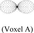
A majority of the previous studies have traditionally calculated the spherical harmonics of the apparent diffusion coefficient (ADC) which is a scaled logarithm of the diffusion measurements. The ADC is useful to describe diffusion in one direction (prolate diffusion). However, for multidirectional diffusion, the ADC profile is no longer similar to the related diffusion probability density function. To demonstrate illogicalness of using ADC or log measurements, two voxels are considered with the horizontal and both of the horizontal and vertical diffusion directions. In addition to the simulation of artificial diffusion signals with SNR=16 and depiction of the profile of the diffusion signal ADC, we calculate their SHC’s and derive the similarity measures between the diffusion signals and ADC’s (Table 1). Note that the SH extracted similarity measure between the two ADC’s is low while it is relatively high for the diffusion signals.
Table 1.
SHC-based similarity between a voxel with the horizontal diffusion direction and its neighboring voxel with both of the horizontal and vertical diffusion directions. The first and second rows show the spherical harmonics representations of the diffusion signal and the related ADC profile, respectively.
| Spherical Representations | Similarity based on SHC | ||
|---|---|---|---|
| Voxel A | Voxel B | ||
| Signal |
|

|
0.9560 |
| ADC Profile |
|

|
0.1519 |
We investigate effects of rotation, elongation, and scale of the diffusion signal and their reflection on the SHC’s. For studying the effect of rotation, an artificial uni-polar diffusion signal is rotated between 0 and 90 degree in 15-degree steps. This rotation is also done on one pole of an artificial bi-polar diffusion signal. Then, the SHC’s of order 8 are computed for each signal. Assuming a reference voxel with one major diffusion orientation (see Table 2), the simulation results show that based on the SHC’s, the similarity between voxels A and B with a major diffusion orientation (with the determined angular difference), is roughly equal to the similarity between voxels A and C where in addition to the major orientation of voxel B, another major diffusion orientation exists. Therefore, the front evolves into that voxel properly.
Table 3.
The effect of rotation, elongation, and scale on the 8th order SH representation of the diffusion signal.
| C20 | Re (C21) | Im (C21) |
| Re (C22) | Im (C22) | |
| C40 | Re (C41) | Im (C41) |
| Re (C42) | Im (C42) | |
| Re (C43) | Im (C43) | |
| Re (C44) | Im (C44) | |
| C60 | Re (C61) | Im (C61) |
| Re (C62) | Im (C62) | |
| Re (C63) | Im (C63) | |
| Re (C64) | Im (C64) | |
| Re (C65) | Im (C65) | |
| Re (C66) | Im (C66) | |
| C80 | Re (C81) | Im (C81) |
| Re (C82) | Im (C82) | |
| Re (C83) | Im (C83) | |
| Re (C84) | Im (C84) | |
| Re (C85) | Im (C85) | |
| Re (C86) | Im (C86) | |
| Re (C87) | Im (C87) | |
| Re (C88) | Im (C88) |
The coefficient invariant to the rotation is remarked by r, to the elongation by e, and to the scale by s.
For studying the effect of elongation, we simulate diffusion signals with linear diffusivity by altering the largest eigen-value of the diffusion tensor. Finally, for studying the effect of scale, diffusion signals with different linear diffusivity are generated by scaling all of the 3 eigen-values. The results are shown in Table 3. Comparing the SHC’s of the linear and planar diffusion profiles, it is illustrated that some of these coefficients are invariant to some of the mentioned effects. Invariant to the rotation (r), invariant to the elongation (e), and invariant to the scale (s) are noted in Table 3.
An important result of the data presented in Table 3 is that the coefficients labeled by “r s e” cannot be used as discriminating features for the diffusion signals. Therefore, they can be removed from the feature space. By modifying the similarity measure in equation (4), the computational cost will decrease. Additionally, by monitoring the changes of these invariant coefficients, we can identify and remove the diffusion outliers. This is achieved when there is a noticeable difference between these invariant coefficients for the neighboring voxels.
b) Application of the Proposed Method to Artificial Data
In order to determine the capability of the proposed method in segmenting fiber bundles, an artificial pattern consisting of three crossing bundles crossed by a circular bundle is created. The diffusion signals and the related ODF are illustrated in Figs. 1–2. As shown in the crossing regions, the diffusion signals (and the ODF which shows the underlying diffusion probability function in the bundles) have two or three major diffusion orientations which can be a good criterion for determining the capability of the method. For comparison, instead of our suggested similarity measure SHCSP in equation (4), some of the similarity measures used previously for tensors like TSP (Tensor Scalar Product) and NTSP (Normalized Tensor Scalar Product) are used in the level set algorithm. These are defined as [17]:
| (7) |
| (8) |
The NTSP shows a superior performance because of its capability to ignore the influence of the relative sizes of the two tensors. Here, we define two more similarity measures: FESP (First Eigen-vector Scalar Product) and FAFESP (FA weighted First Eigen-vector Scalar Product).
| (9) |
| (10) |
Fig. 1.

Illustration of the diffusion signals for an artificial crossing pattern.
Fig. 2.

Illustration of the ODF’s of the artificial crossing pattern representing the underlying diffusion probability function in the bundles.
To quantify the results, a correctness measure is calculated for the segmentation results using the following relation:
| (11) |
where the So and Sr are the target and resulting structures, respectively, and N is the number of voxels laying in each structure. Here, N(So ⌒ Sr) and are number of the True-Positive and False-Positive voxels, respectively.
In order to prevent the front to propagate from a bundle to a neighboring bundle, we modify the speed function by adding a prevention term based on the similarity between the main diffusivity directions of the neighboring voxels, obtained from an ODF maximum finding procedure [21]. This modifies equation (4) to:
| (12) |
where ‘i’ is the current voxel on the boundary of the propagating front, ‘i+1′ is the neighboring voxel pointed to by the normal to the front direction at the voxel ‘i’ in the 27-voxel neighborhood system and ‘fdd’ and ‘sdd’ stand for the first and second diffusion directions, respectively. Then, the resulting similarity measure is normalized and a threshold is applied to remove minor speed terms obtained from low similarities which can make the algorithm unstable. We call this modified similarity measure “Spherical Harmonic Coefficients Scalar Product (SHCSP).”
To see the results of applying different similarity measures for crossing fiber bundles, look at Fig. 3 which illustrates the segmentation steps from a seed voxel to the final step using tensor-based, SHC-based through equation (4) and SHC-based through equation (12) similarities. In this figure, the headless arrows and the colors red, light green, and dark green show directions and color-coding of the principal diffusion directions, respectively, while the gray color represents the segmented area. As shown in the top row, a tensor-based similarity between the neighboring voxels fails to propagate inside the crossing areas. The reason is that there is a minor similarity between a prolate tensor inside the bundle to be segmented and an oblate or a spherical tensor (fitted to the diffusion measurements) inside the crossing bundle.
Fig. 3.

Illustration of the segmentation steps from seed voxel to final step. Top: using tensor-based similarity. Middle: using SHC-based similarity through equation (4) like the result of [20]. Bottom: The proposed algorithm using SHC-based similarity through equation (12) (desired segmentation steps). The headless arrows and the colors red, light green, and dark green show directions and color-coding of the principal diffusion directions, respectively, while the gray color represents the segmented area.
The middle row shows that by using SHC-based similarity through equation (4), the front propagates properly inside the crossing area. This is because the scalar product between the SHC’s of a voxel inside the bundle to be segmented and the voxel in the crossing area is high as discussed in section IIIa. However, because the scalar product between the SHC’s of a voxel inside the crossing area and the voxel inside the crossing bundle (which we do not like to segment) is again high, the front propagates improperly inside the crossing bundle. This satiation makes the method of Descoteaux and Deriche useless, as it cannot isolate and segment individual fiber bundles; instead it segments all of the crossing bundles as a single object. Our proposed method avoids this situation by using SHC-based similarity through equation (12) which adds a preventing term based on the similarity between the neighboring principal diffusion directions.
The proposed segmentation algorithm starts from a voxel with one major diffusion direction, then, compares this direction with the main diffusion directions in the next voxel (pointed to by the normal direction of the voxel). Next, the most collinear direction is kept while the remaining major directions in the next voxel are removed. In addition, it propagates the front based on the similarity, if there is a pair with high similarity (collinearity). Therefore, in each voxel inside the segmented bundle, there is only one principal diffusion direction parallel to the diffusivity direction in that bundle.
Now, look at the bottom row of Fig. 3 which illustrates the segmentation steps from the seed voxel to the final step using the proposed algorithm based on SHC-based similarity through equation (12). Note that the front propagates properly inside every crossing area and after passing through each, it continues propagating to the remaining parts of the desired bundle until reaching its end. In this way, it segments the entire bundle without penetrating inside the crossing fibers except for the crossing area that is shared between them.
We utilize the level set framework and define its speed function term based on the above similarity measure. For the local dependence, the similarity measure is calculated between every voxel on the propagating surface and its neighbors in the propagation direction. The speed function term moves the front to fill the whole fiber bundle. The regularizing curvature term in equation (6) is in charge of smoothing the fiber bundles without changing their tubular structures. It is shown that our method has advantages over the methods that use similarity measures based on the DTI, by properly propagating the front in the fiber crossing areas where a scalar value such as an anisotropy measure, or even the whole information contained in the fitted tensor, fails to separate them.
We have implemented the proposed algorithm in MATLB R2008a using a PC with Intel® Core™ 2Due CPU (E8400@3.00GHz, 3.00GHz) and 4GByte RAM and 64 bit VISTA operating system. The results of the level set algorithm using five similarity measures (TSP, NTSP, FESP, FAFESP and SHCSP) are presented in Table 4 and Fig. 4. Note that the proposed method is robust against noise. The SNR values where the algorithm is sensitive to noise are between 12 to 32 while the other methods (TSP, NTSP, FESP, and FAFESP) are sensitive to noise even in the high SNR values between 110 to 150. This is because of the implicit smoothing in the SHC fitting to the diffusion signals. Moreover, the proposed SHCSP method achieves a 100% correctness at SNR = 32, which is superior to the best result of the tensor-based methods obtained by FAFESP at SNR = 150. Although the false positive rate is zero, the number of true positives does not reach the number of voxels in the diffusive pattern, because of inability of the tensor-based methods to propagate into the crossing regions. Fig. 4 shows that the correctness of the proposed method (SHCSP) is 100% for the SNR ranges that the tensor based methods are sensitive to noise. The NTSP and FAFESP methods are superior in the low and high SNR ranges, respectively.
Table 4.
Correctness of the segmentation results for each of the methods. Top: Results of the proposed method based on the SHCSP similarity. Bottom: Best results of the tensor -based methods.
| SNR | nP | nTP | nFP | Correctness | Final Time (Sec) |
|---|---|---|---|---|---|
| 12 | 21504 | 12272 | 9232 | 24.8% | 1831.6 |
| 16 | 20779 | 13028 | 7751 | 40.5% | 1077.4 |
| 20 | 21293 | 15857 | 5436 | 65.7% | 1138.1 |
| 24 | 20170 | 15585 | 4585 | 70.1% | 1290.6 |
| 28 | 20012 | 17451 | 2561 | 85.3% | 1221.3 |
| 32 | 21080 | 21080 | 0 | 100% | 1219.6 |
| SNR | nP | nTP | nFP | Correctness | Final Time (Sec) |
|---|---|---|---|---|---|
| 100 | 18115 | 11094 | 7021 | 19.3% | 1082.9 |
| 110 | 18880 | 13397 | 5483 | 37.5% | 778.5 |
| 120 | 18523 | 14491 | 4032 | 49.6% | 635.5 |
| 130 | 17536 | 15541 | 1995 | 64.2% | 669.0 |
| 140 | 18296 | 17743 | 553 | 81.5% | 677.8 |
| 150 to ∞ | 18124 | 18124 | 0 | 86.0% | 678.6 |
Fig. 4.

Correctness of the results obtained by five different methods (TSP, NTSP, FESP, FAFESP, and SHCSP) for different ranges of SNR’s (12, 16, 20, 24, 28, 32, 100, 110, 120, 130, 140, 150). Top: Comparison of different methods as a function of SNR. The vertical axis shows the correctness and the horizontal axis shows the SNR’s. Bottom: Comparison of each method’s performance as a function of SNR. The vertical axis shows correctness and the horizontal axis shows the methods. Note that the proposed method (SHCSP) is 100% accurate for the SNR ranges in which the tensor based methods are sensitive to noise. After the proposed method, NTSP and FAFESP show superior performance compared to TSP and FAFESP in the low and high SNR ranges, respectively.
c) Application of the Proposed Method to Real Data
In order to apply the proposed method to real HARDI MRI data, a normal subject was scanned by a GE Signa Excite1.5T MRI system (General Electric Medical Systems, Milwaukee, WI, USA) in Stanford Lucas Imaging center through a Q-ball Imaging protocol with a 492 diffusion synthesizer gradient scheme and 13 B0 reference images with imaging volume dimension of 128×128×33 and imaging voxel dimension of 1.95×1.95×4.5 mm.
After smoothing the data using a Gaussian kernel, registering diffusion images on a reference volume, resizing the data to a finer grid of 1×1×1 mm (better suited for the level set algorithm) and reordering of the diffusion signals from scanner-wise to voxel-wise order, we calculate the SHC’s with order of 8 for every voxel of the diffusion signal using the equations introduced in the previous sections.
For segmentation, multiple seed points from each fiber bundle should be specified. For this reason, our segmentation algorithm is semi-automatic. This is performed by computing the FEFA (First Eigen-vector weighted by Fractional Anisotropy) map and comparing it with an atlas that includes major fiber bundles [27]. As mentioned previously, by calculating the similarity measure between the neighboring SHC’s, the speed function of the level set framework is obtained. Note that it is not mandatory to calculate the speed function in all voxels, since the front propagation in each step depends on the speed function of the boundary points only. However, this function is specified in a wide-enough stripe, e.g., with 3 points around the boundary [26].
The segmentation results of the proposed algorithm for major fiber bundles like Corpus Callosum (CC), Cingulum (Cg), and Cortico-Spinal tract (CST) are shown in Figs. 5–8. They illustrate that the algorithm is capable of isolating these fiber bundles from the HARDI data. The results for CC and CST tracts for tensor-based segmentation with NTSP as the similarity measure [17] (as the best tensor-based segmentation method in the literature) are shown in Figs. 5–6. Note that the tensor-based segmentation fails to find the entire fiber bundle and is sensitive to the threshold and the initial seeds while our proposed method reconstructs the entire structure of these bundles in less-sensitive semi-automatic manner.
Fig. 5. Comparison of segmentation results of the Corpus Callosum (CC) tract obtained by two models.

Top row: The results of the tensor-based method in [17] for different thresholds. Middle row: The results of our implementation of the tensor-based method in [17] for different threshold levels. Bottom row: The results of the proposed algorithm in different views.
Fig. 8.

Segmentation results (in different views) for the CC (violet), tapetum (red), Cgu (cyan), CST (green) tracts obtained by the proposed algorithm.
Fig. 6. Comparison of Cortico-Spinal (CST) tract segmentation results obtained by two models.

Top row: The results of the tensor-based method in [17] for different threshold levels. Bottom 2 rows: The results of the proposed algorithm in different views.
Fig. 5 compares the segmentation results of the Corpus Callosum (CC) obtained by two models. In the top row, the segmentation results obtained by the tensor-based segmentation method proposed in [17] for different threshold levels are presented. In the middle row, the results of our implementation of the tensor-based segmentation method of [17] for different thresholds are shown. In the bottom row, the segmentation results obtained by our proposed algorithm are illustrated. Note that they cover the entire CC, are consistent with the neuro-anatomy of the brain, and are not sensitive to the threshold. Moreover, they do not penetrate into the neighboring bundles like Cingulum, Tapetum, Superior Fronto-Occipital Fasciculus, Superior Longitudinal Fasciculus, and Inferior Longitudinal Fasciculus.
Fig. 6 shows the segmentation results of CST obtained by two models. In the top row, the segmentation results obtained by the tensor-based segmentation in [17] for different thresholds are presented. In the two bottom rows, the segmentation results obtained by our proposed algorithm are illustrated which cover the entire CST consistent with the neuro-anatomy of the brain, and are not sensitive to the threshold level.
Fig. 7 illustrates the segmentation results obtained by our proposed algorithm which cover the entire Cg and are consistent with the neuro-anatomy of the brain. Here, again the front does not penetrate into the neighboring bundles like CC. These segmented fiber bundles and the Tapetum fiber tract again as a fiber bundle that is a neighbor of the CC, are illustrated in Fig. 8. Note that there are areas shared between the bundles where the proposed algorithm succeeded to pass through and continue to find the individual bundles.
Fig. 7.

Segmentation results for the Cingulum (Cg) tract obtained by the proposed algorithm and shown in different views.
IV. Conclusions
In this paper, we have presented a novel semi-automatic method for segmenting the fiber bundles. The proposed method calculates spherical harmonic coefficients and uses them for defining a similarity measure as the speed function term in the Hamilton-Jacobi equation of the level set framework. We have shown that our method has advantages over methods using similarity measures based on the DTI. These advantages have been achieved by a proper propagation of the front within the fiber crossing areas without any assumptions about the diffusivity profile or model and by dealing with the diffusion signals. Our simulation results have shown the capability of the proposed method in detecting crossing bundle patterns even in low SNR conditions. We have demonstrated the segmentation results of the experimental HARDI data for extracting three major fiber bundles of the brain (corpus callosum, cingulum, and cortico-spinal tracts).
Extraction of the fiber bundles makes it possible to quantify the diffusion characteristics in each bundle and opens new perspectives for monitoring disease evolution. For example, it can be used to evaluate the diffusion characteristics inside the splenium of the corpus-callosum in Schizophrenic patients and the genu of the corpus-callosum in alcoholics. Furthermore, the neurologists can evaluate the therapy effects and map important brain connections that should be preserved during surgical interventions. In addition, the distinct fiber bundles can be used in the fiber tracking algorithms to avoid propagation of the fibers from a specific bundle to the others. This may be achieved by using the segmentation results as a regularization term. Furthermore, they can be used to access the white matter mask composed of them.
Our method benefits from the smoothing property of the SH representation to reduce the effect of the imaging noise on the segmentation results. In addition, the proposed method is robust against crossing, branching, and merging of the bundles. In the future, we plan to use the SH representation as a powerful feature descriptor in other segmentation frameworks beyond the level set.
Table 2.
Illustration of artificial linear and planar diffusion signals in voxels B and C, respectively, using the SHC’s in the spherical coordinates and their similarities with a reference signal in voxel A.
| Similarity between Reference Signal and Signal of Left Column | Bi-Modal Diffusion Signal (Voxel C) | Similarity between Reference Signal and Signal of Left Column | |||
|---|---|---|---|---|---|
| Rotation Angle (Degrees) | Uni-Modal Diffusion Signal (Voxel B) | Signal Profiles from 2 tensors | Combined Signal Profile | ||
| 0 |
|
1.000 |

|

|
0.956 |
| 15 |

|
0.7620 |

|

|
0.7616 |
| 30 |

|
0.3621 |

|

|
0.3543 |
| 45 |

|
0.1508 |

|

|
0.1470 |
| 60 |

|
0.0659 |

|

|
0.0628 |
| 75 |

|
0.0250 |

|

|
0.0246 |
| 90 |
|
0.0195 |
|

|
0.0195 |
References
- 1.Basser PJ, Mattiello J, Le Bihan D. MR diffusion tensor spectroscopy and imaging. Biophysical. 1994;66:259–267. doi: 10.1016/S0006-3495(94)80775-1. [DOI] [PMC free article] [PubMed] [Google Scholar]
- 2.Basser PJ, Mattiello J, Le Bihan D. Estimation of the effective self-diffusion tensor from the NMR spin echo. Journal of Magnetic Resonance. 1994;103:247–254. doi: 10.1006/jmrb.1994.1037. [DOI] [PubMed] [Google Scholar]
- 3.Tuch DS, Di_usion . PhD thesis. Harvard University and Massachusetts Institute of Technology; 2002. MRI of complex tissue structure. [Google Scholar]
- 4.Tuch DS, Reese TG, Wiegell MR, Makris NG, Belliveau JW, Wedeen VJ. High angular resolution diffusion imaging reveals intravoxel white matter fiber heterogeneity. Magn Reson Med. 2002 doi: 10.1002/mrm.10268. [DOI] [PubMed] [Google Scholar]
- 5.Tournier J-D, Calamante F, Gadian DG, Connelly A. Direct estimation of the fiber orientation density function from diffusion-weighted mri data using spherical deconvolution. NeuroImage. 2004;23:1176–1185. doi: 10.1016/j.neuroimage.2004.07.037. [DOI] [PubMed] [Google Scholar]
- 6.Dell F, Acqua, Rizzo G, Scifo P, Clarke RA, Scotti G, Fazio F. A model-based deconvolution approach to solve fiber crossing in diffusion-weighted mr imaging. IEEE Transactions in Biomedical Engineering. 2007;54(3):462–472. doi: 10.1109/TBME.2006.888830. [DOI] [PubMed] [Google Scholar]
- 7.Alexander DC. Maximum entropy spherical deconvolution for diffusion MRI. Image Processing in Medical Imaging. 2005:76–87. doi: 10.1007/11505730_7. [DOI] [PubMed] [Google Scholar]
- 8.Jansons KM, Alexander DC. Persistent angular structure: new insights fom diffusion magnetic resonance imaging data. Inverse Problems. 2003;19:1031–1046. [Google Scholar]
- 9.Tuch DS. Q-Ball imaging. Magn Reson Med. 2004;52:1358–1372. doi: 10.1002/mrm.20279. [DOI] [PubMed] [Google Scholar]
- 10.Brun A, Knutsson H, Park HJ, Shenton ME, Westin CF. Clustering fiber traces using normalized cuts. MICCAI 2004, LNCS 3216. 2004:368–375. doi: 10.1007/b100265. [DOI] [PMC free article] [PubMed] [Google Scholar]
- 11.Maddah M, Grimson WEL, Warfield S, Wells WM. A unified framework for clustering quantitative analysis of white matter fiber tracts. Med Imag Analysis. 2008;12:191–202. doi: 10.1016/j.media.2007.10.003. [DOI] [PMC free article] [PubMed] [Google Scholar]
- 12.Zhukov L, Museth K, Breen D, Whitaker R, Barr A. Level Set modelling and segmentation of DT-MRI brain data. J Electron Imag. 2003;12:125–133. [Google Scholar]
- 13.Vemuri B, Chen Y, McGraw T, Wang Z, Mareci T. Fiber tract mapping from diffusion tensor MRI. Proceedings of the IEEE Workshop on Variational and Level Set Methods in Computer Vision. 2001:81–88. [Google Scholar]
- 14.Wang Z, Vemuri B. ECCV, LNCS 3024. Springer; Berlin: 2004. Tensor field segmentation using region based active contour model; pp. 304–315. [Google Scholar]
- 15.Rousson M, Lenglet C, Deriche R. Level set and region based surface propagation for diffusion tensor MRI segmentation. CVAMIA and MMBIA. 2004 [Google Scholar]
- 16.Feddern C, Weickert J, Burgeth B. Level-Set methods for tensor valued images. Proceedings of the Second IEEE Workshop on Variational, Geometric and Level Set Methods in Computer Vision. 2003:65–72. [Google Scholar]
- 17.Jonasson L, Bresson X, Hagmann P, Cuisenaire O, Meuli R, Thiran J. White matter fiber tract segmentation in DT-MRI using geometric flows. Medical Image Analysis. 2005;9(3):223–236. doi: 10.1016/j.media.2004.07.004. [DOI] [PubMed] [Google Scholar]
- 18.Jonasson L, Hagmann P, Bresson X, Thiran JP, Wedeen VJ. Representing diffusion MRI in 5D for segmentation of white matter tracts with a level set method. IPMI. 2005:311–320. doi: 10.1007/11505730_26. [DOI] [PubMed] [Google Scholar]
- 19.Hagmann P, Jonasson L, Deffieux T, Meuli R, Thiran JP, Wedeen VJ. Fibertract segmentation in position orientation space from high angular resolution diffusion mri. NeuroImage. 2006;32:665–675. doi: 10.1016/j.neuroimage.2006.02.043. [DOI] [PubMed] [Google Scholar]
- 20.Descoteaux M, Deriche R. Segmentation of Q-Ball Images Using Statistical Surface Evolution,” MICCAI 2007/Brisbane Australia. 2007 Oct; doi: 10.1007/978-3-540-75759-7_93. [DOI] [PubMed] [Google Scholar]
- 21.Hess CP, Mukherjee P, Han ET, Xu D, Vigneron DB. Q-ball reconstruction of multimodal fiber orientations using the spherical harminic basis. Magn Reson Med. 2006;56:104–117. doi: 10.1002/mrm.20931. [DOI] [PubMed] [Google Scholar]
- 22.Descoteaux M, Angelino E, Fitzgibbons S, Deriche R. Regularized, fast and robust analytical Q-Ball imaging. Magn Reson Med. 2007;58:497–510. doi: 10.1002/mrm.21277. [DOI] [PubMed] [Google Scholar]
- 23.Mousa M, Chaine R, Akkouche S. Frequency-Based representation of 3D Models using spherical harmonics. The 14-th International Conference on Computer Graphics, Visualization and Computer Vision. 2006;14:193–200. [Google Scholar]
- 24.Mousa M, Chaine R, Akkouche S, Galin E. Efficient spherical harmonics representation of 3D objects. PG′07, Pacific Graphics conference, Maui, USA. 2007 [Google Scholar]
- 25.Osher S, Sethian J. Fronts propagating with curvaturedependent speed: algorithms based on Hamilton–Jacobi formulations. J Comput Phys. 1988;79:12–49. http://www.citeseer.nj.nec.com/osher88fronts.html. [Google Scholar]
- 26.Osher S, Fedkiw R. Level Set methods and dynamic implicit surfaces. Springer-Verlag New York. 2002 [Google Scholar]
- 27.Wakana S, Jiang H, Nagae-Poetscher LM, van Zijl PCM, Mori S. Fiber Tract–based Atlas of Human White Matter Anatomy. Radiology. 2004 Jan;230:77–87. doi: 10.1148/radiol.2301021640. [DOI] [PubMed] [Google Scholar]