Estimating adult sex ratios in nature

Abstract

Adult sex ratio (ASR, the proportion of males in the adult population) is a central concept in population and evolutionary biology, and is also emerging as a major factor influencing mate choice, pair bonding and parental cooperation in both human and non-human societies. However, estimating ASR is fraught with difficulties stemming from the effects of spatial and temporal variation in the numbers of males and females, and detection/capture probabilities that differ between the sexes. Here, we critically evaluate methods for estimating ASR in wild animal populations, reviewing how recent statistical advances can be applied to handle some of these challenges. We review methods that directly account for detection differences between the sexes using counts of unmarked individuals (observed, trapped or killed) and counts of marked individuals using mark–recapture models. We review a third class of methods that do not directly sample the number of males and females, but instead estimate the sex ratio indirectly using relationships that emerge from demographic measures, such as survival, age structure, reproduction and assumed dynamics. We recommend that detection-based methods be used for estimating ASR in most situations, and point out that studies are needed that compare different ASR estimation methods and control for sex differences in dispersal.

This article is part of the themed issue ‘Adult sex ratios and reproductive decisions: a critical re-examination of sex differences in human and animal societies’.

1. Introduction

The adult sex ratio (ASR) is a demographic property of a population that emerges from differences in sex ratio at birth, sex differences in juvenile or adult mortality, or sex differences in maturation times and dispersal patterns [1,2]. Variation in ASR profoundly influences many aspects of behaviour, including mate acquisition, sex roles and parental care, because the rarer sex in the adult population has more potential partners to mate with than the supernumerary sex [3–5]. Unbalanced ASRs may also affect lifetime reproductive success or survival probabilities [6–10] by increasing investment in mate competition, sexual harassment or parental care [9–11].

The ASR also plays a crucial role in population dynamics [9,12–14] and biodiversity conservation [15–17]. For example, strongly biased ASRs influence the risk of extinction or population collapse [9,18–21] and affect fishery quotas, bag limits and harvestable populations in game animals [22,23]. Finally, recent studies of humans show that the ASR may also influence partner choice, demography and economic decisions [24,25], which could have important socioeconomic and biological consequences in human populations [26]. Thus, obtaining accurate ASR estimates is essential for studies in evolutionary and behavioural biology, population ecology, biodiversity conservation, resource management and the social sciences.

Like numerous other demographic and population parameters measured in the field, obtaining accurate ASR estimates can be challenging. In human populations, the ASR (often referred to as the population sex ratio) is generally estimated from census data [27], and although these data are often of good quality, they are not free of errors [28]. Censuses may miss or double-count one sex more frequently than the other (e.g. if migration rates, privacy concerns or misreporting of age differ between men and women) and these miscounts are expected to lead to distortions in (age-specific) sex ratio estimates [29].

In wild animal populations, the ASR is estimated through encounters with live or dead individuals, either by counting or capturing them, and obtaining accurate ASR estimates may be particularly challenging. First, in sexually monomorphic species where genitalia are not visible (e.g. birds and some anuran species), recognizing males and females may require the application of DNA-based sexing with tissue samples obtained [17,30]. Second, males and females often have different behaviour, which may result in sex differences in detectability [31–33]. Males from sexually dimorphic animals are often visually more ornamented or vocally more active (e.g. orang-utans, howler monkeys, songbirds, lizards and butterflies) and therefore, easier to detect than females, so the number of males relative to females could be overestimated [34,35]. Third, biases in the estimation of the ASR may result from failure to detect non-breeding adults (i.e. floaters), which often remain unnoticed because they have less conspicuous lifestyles, are more mobile or live at the margins of a population [2,36,37]. For example, in highly polygynous species such as northern elephant seals (Mirounga angustirostris), females congregate on breeding beaches, whereas only a few males—the beach masters—mix with them, although many mature males patrol around the breeding colony but they rarely come on land [38]. ASR estimation can be further complicated if males and females segregate into different habitats or use different microhabitats at certain times of the year, which occurs in many terrestrial, volant and aquatic species [39–41]. Finally, spatial distributions and aggregations often vary between the breeding and non-breeding seasons, and thus, different methodologies may be required to estimate male versus female numbers during different seasons [4,42,43].

Here, we review and evaluate measures and methods of estimating the ASR in wild animal populations. We have four main objectives. First, we present an overview of the different measures used to estimate the ASR in wild populations and evaluate their relative merits and limitations. Second, we investigate how differences between the sexes in detectability or catchability may introduce bias in ASR estimates. Third, we discuss recent statistical advances that can be applied to account for the factors affecting ASR estimates and how they vary in space and time. Finally, we recommend topics for future research. We focus on dioecious animals, although we recognize that male and female functions show fascinating variation in hermaphrodites [44], and that ASR estimation is also important for ecological and evolutionary inferences in plants [45–47].

2. Measures of the adult sex ratio

The ASR is one of the six types of sex ratios (figure 1) that traditionally have been used to describe a population [48] and that vary according to the age profile of the population : primary sex ratio (i.e. sex ratio at fertilization), secondary sex ratio (i.e. sex ratio at birth or hatching), tertiary sex ratio (i.e. sex ratio of sexually mature individuals), operational sex ratio (OSR), quaternary sex ratio (i.e. sex ratio of post-reproductive organisms) and ASR, which is the sex ratio of all individuals beyond the age of maturation. The OSR refers to the subset of adults that are sexually active and is usually expressed as the ratio of sexually active males to females [49]. OSR has often been confused with ASR, although they are conceptually different: ASR refers to all individuals that have reached the age of sexual maturation whether sexually active or not [2,50], whereas OSR is determined by the number of males and females that are available and actively seeking mates (which excludes sexually inactive and parenting adults [4]) and reflects the availability of partners (i.e. mating opportunity [51]).

Figure 1.

Proposed terminology for sex ratios. Modified from [4]. Note that ‘mature’ means reaching the minimum age of first breeding, and the category of ‘post-breeding’ adults includes those males and females who survive beyond reproductive cessation. SR, sex ratio.

This typology for characterizing sex ratios was adequate for decades, but it has limitations. First, two important life-history stages have been left out: sex ratio of young at independence and sex ratio at maturation (MSR), which influence the transition rate of individuals into the adult or operational classes. The ecological and demographic processes operating during these stages may differ profoundly from the ones affecting pre-birth and post-birth, and therefore, there is a need to recognize the importance of these key life-history stages (figure 1). However, these data can be extremely hard to collect and this may be the reason why these two stages have been overlooked. Second, sex ratios at fertilization, birth, independence and maturation can be considered snapshots of a given age cohort, whereas the ASR and the post-breeding sex ratio are calculated over multiple cohorts consisting of the relevant age classes. Analogous to the ASR and the quaternary sex ratio, we propose that juvenile sex ratio should refer to the sex ratios at post-birth and pre-independence of the offspring (figure 1).

Operationally, the ASR should include all adult males and females that have reached reproductive age. Most ASR estimates from wild animal populations do not usually distinguish between reproductive and post-reproductive adults because this is often difficult to do. Differences in reproductive lifespan between males and females in humans [52] and in many cetacean and insect populations [53] would be reflected in estimates of tertiary sex ratio.

Sex ratios (including the ASR) have been expressed in numerous ways. The first is as a proper ratio of males to females (e.g. 2 M : 1 F and 1 M : 2 F), which can be readily converted to a real number (e.g. 2.0 or 0.5, respectively). The ratio-based expression of ASR, however, is problematic because it is bounded by zero on one end, but is not bounded at the other end (i.e. positive infinity). As a consequence, the ratio is asymmetric around 1.0, and the same extent of male-versus female-bias leads to a very different scaling towards zero or towards positive infinity.

Second, social scientists and game biologists often express the ASR as the number of males relative to 100 females (e.g. [22,27]). So a male-biased ASR (i.e. more than 100 males relative to 100 females) refers to a ‘high’ sex ratio, whereas female-biased ASR refers to a ‘low’ sex ratio. Expressing the ASR in this way has the same problems as the proper ratio discussed above: asymmetry and different lower and upper boundaries.

In dioecious populations, the ASR has two natural limits: all males or all females. Therefore, expressing the ASR as the proportion of one sex (conventionally, the male) in the total adult population (males plus females) has the ability to capture the full range of biological variation and, moreover, it produces a metric that is symmetrical around 0.5 (half males and half females). Although it would be tempting to devalue extreme ASRs in either direction and express the ASR as the log of the number of males divided by the number of females, which is analogous to the way that sexual size dimorphism is often expressed [54] (but see [55]), this approach would result in an asymmetric measure that is not easily interpretable on one end and infinite on the other end.

We therefore strongly recommend using the proportion of males in the adult population as a general measure of the ASR (i.e. ASR = N_males/(N_males + N_females)), because it is bounded between 0 (only females in the population) and 1 (only males in the population). This measure of the ASR is easy to interpret for two reasons. First, it does not invoke individuals of one sex as fractions of individuals of the other sex, so it is more in accordance with the nature of individuals as discrete units. Second, it results in values between 0 and 1 that reflect the relative abundances of males and females in the adult population.

In summary, we suggest that the proportion of males in the adult population is the preferred estimator of the ASR. Expressing the ASR as a ratio in the strict sense (e.g. males to females, or females to males) or as the total number of males per 100 females is problematic because these measures are unbound on the upper end and tend to be asymmetric. Using the proportion of males in the population of interest (figure 1) as a standard expression of the sex ratio can be a way to further integrate sex ratio research across different disciplines.

3. Factors differentially affecting the detection and capture of males and females

The basic unit of measurement for the ASR is a count of live or dead individuals that are either observed or captured. If there are differences in the behaviour and conspicuousness of males and females, this could affect the observation or capture process and can bias any estimate of sex ratio. Here, we discuss these possible differences and their effects on sex ratio estimation.

Males and females often differ in morphology (e.g. size and colour) and behaviour (e.g. vocalization frequency or intensity, cautiousness, foraging habits, home range size or sociality) that can make one sex more likely to be detected or captured [33,56,57]. ASR estimates that disregard potential differences in detectability or catchability between males and females are likely to be biased towards the more conspicuous or catchable sex [17,33,34]. For example, in several ungulate populations, males are more difficult to spot and therefore to count because they are solitary or occur in smaller groups, tend to forage in areas with taller and thicker vegetation, or are more wary of the presence of human observers than females [31,58,59]. These differences in behaviour can bias sex ratio estimates of ungulate populations towards females [58,60]. Similar bias may also occur in other species where females are more trappable than males due to sex differences in activity patterns (e.g. in the Central American spiny rat Proechimys semispinosus [61]).

Conversely, bias in ASR estimates towards males may exist in many animal populations where males are easier to detect or catch than females [33]. In most songbird populations, for example, males may be more easily detected (and counted) than females due to their brighter plumage colours and their noticeable visual and vocal displays associated with territorial defence [62,63]. Male songbirds can also be surveyed or caught more frequently because they have larger home ranges or are more prone to prospect new territories than females, or because females often take care of all incubation duties, causing them to be on nests and unavailable for detection [34]. Sex differences in the size of the home range or in territorial and dominance behaviour that make males easier to detect or capture than females can also occur, as, for example, in shorebirds [64] and small and medium-sized mammals such as mice, lemmings and raccoons [65–67].

Other behavioural differences may also lead to sexual segregation and sex differences in detectability or catchability that should be considered when estimating the ASR. In the flatfish Pleuronectes platessa, males are more active during the spawning period and spend more time on spawning grounds than females, and these differences can give rise to a predominance of males in commercial catches and measurement bias in the ASR towards males [68]. Sex differences in breeding durations are expected to lead to sex differences in detectability or catchability and result in an ASR estimate that is biased [69], although their contribution to these quantities has rarely been estimated. In migratory species, potential differences between the sexes in detection and capture probabilities arise because males and females may exhibit differences in arrival dates and duration at stopover sites and breeding grounds, or may over-winter in separate areas or use different migration routes [43,70]. Therefore, counts obtained from stopover sites risk producing estimates that may not reflect the sex ratio of a population as a whole, but instead reflect sex differences in migratory patterns [71]. Furthermore, when species exhibit sexual segregation with regard to habitat, site-specific detection and capture probabilities can be biased towards the sex concentrated in the habitat where detection or capture is favoured, even if encounter probabilities are otherwise equal between the sexes [63].

ASR estimation can be further complicated by phenological variation in sex-specific traits (e.g. changes in behaviour and morphology associated with reproduction [72]), or by differences in the frequency with which males and females skip breeding events [42,73], especially when non-breeding adults of either sex often remain undetected [36,37]. Accounting for variable detectability between the sexes can be complex in monomorphic species, especially in cases where sex can only be determined by molecular techniques or dissection [30].

Selective effects of trapping methods or baits may also lead to sex differences in detectability or catchability and bias ASR estimates (reviewed in [74]). For example, male mirid bugs (family Miridae) are more strongly attracted to light-traps than females and this difference is accentuated when ultraviolet traps are used, because males seem to be more attracted to UV light-traps than to tungsten filament light-traps [75]. Similarly, trapping methods may lead to marked sex differences in catchabilities and bias in ASR estimates. In the European serin Serinus serinus, baited platform traps capture fewer females than males in comparison to clap nets, probably because dominant males monopolize the baited surface of platform traps [57]. In the fiddler crab Uca pugilator, males are captured more frequently than females in foraging areas than within burrows, and sex ratio estimates are strongly affected by the type of sampling and trapping method that is used [76]. Spatial positioning of traps may also generate bias in detectability and sex ratio estimates. For instance, pheromone-baited traps placed in the top of trees may catch a higher number of male moths than those placed in lower canopy positions, and these effects of trap positioning may have important implications for estimations of population dynamics and pest management decisions [77].

While biases to the ASR due to these different potential sources of errors are often unmeasured, making the accuracy of ASR estimates from the wild difficult to assess, ASR estimates from wild populations suggest reasonable precision when compared across species. In birds that have several published ASR estimates, the intra-class correlation was highly significant (figure 2a). Note that this is not repeatability in the strict sense because the estimators for a given species were often from a different population and/or from different time periods. Similarly, ASRs that were collected for a given species by different estimation methods were also significantly correlated (figure 2b).

Figure 2.

Intra-class correlation in ASR in bird species that have (a) several ASR estimates (up to six estimates per species, r_ICC = 0.643, F = 6.40, p < 0.001, n = 57 species) or (b) obtained by different methods (r_ICC = 0.717, F = 6.469, p < 0.001, n = 18 species). Methods were classified into six categories: counting breeding adults in individually marked populations, counting non-breeding adults, capturing breeding or non-breeding birds, demographic modelling, counting dead birds and counting birds in museum collections. Horizontal dashed line denotes unbiased ASR (value = 0.50) (A. Liker & T.S. 2017, unpublished data).

4. Detection-based methods of estimating the adult sex ratio from unmarked individuals

The multitude of factors discussed above that can differentially affect the detection and capture of males and females, and therefore lead to measurement errors, can be accounted for through the application of statistical methods to yield less biased estimators of the ASR. In the next three sections, we review these approaches. We begin our examination of ways to account for detection differences between the sexes by exploring methods to account for detection bias for the most common type of data used in sex ratio estimation: counts of unmarked males and females in a population. These counts typically come from direct observations of unmarked individuals alive and counted in the field, trapped, killed by collisions (e.g. with vehicles or buildings), or shot by hunters and caught by fishermen. The approaches described in this section illustrate some of the possibilities for ASR estimation when sampling unmarked populations that can be sexually identified in the field. In addition, we refer readers to a method that may be useful to handle uncertain observations where sex is unknown for some individuals.

The past two decades have seen the development of several statistical methods to account for detection error in the counts of unmarked populations, i.e. when animals are not individually identified (reviewed in [78,79]). This is accomplished by: (i) jointly modelling abundance (often as a Poisson distribution) and the detection probability of each individual (often as a binomial distribution) using hierarchical models that require temporal replication in counts [80,81]; (ii) by using ancillary data such as the distance to the detected individual(s) to develop a detection function [82]; or (iii) by modelling detection as a function of site-specific covariates using a conditional likelihood model when sites were only visited once [83].

Detection-based approaches to estimate the ASR would apply one of the modelling approaches discussed above to counts of unmarked individuals of each sex to generate separate estimates of the abundance of males and females for each sampling unit. These estimates of male and female population size are then used to obtain the ASR. Detection-based ASRs can be compared among different localities, seasons or years by including spatial and temporal components as factors in the models. The ASR calculated from the abundance estimates corrected for detectability is, in principle, less biased than using ASR estimates derived from raw counts when detection varies between sexes, sites or surveys.

An emerging approach to model count data for imperfect detection combines a binomial generalized linear model (GLM) and a standard Poisson GLM [80]. Counts at site i are regarded as a binomial process dependent upon the detection probability p (i.e. the observation process) and N_i is a Poisson random variable (i.e. the state process):

2.1

where N_i is the abundance at site i and λ the expected abundance (i.e. the mean abundance over all sites). C_ij is the count at site i during survey j and p is the individual detection probability. This is the standard formulation of the widely used N-mixture model for analysing counts to derive a population estimate [79]. Additional explanatory variables can be included in both the abundance and the detection models using standard generalized linear modelling techniques. Box 1 illustrates how this type of detection-based method accounts for detection probability and can generate ASR estimates that are less biased than non-detection-based approaches (i.e. using raw count data). As detection-based models allow researchers to investigate how abundance varies according to environmental factors [79,80], these methods provide the ability not only to generate estimates of the ASR but could be used to directly assess how different factors influence the ASR of populations.

Box 1. Estimating the ASR of unmarked populations: a simulation exercise.

We simulated random populations of males and females for i = 50 sites with a Poisson mean of 10 individuals (five males + five females) using a true (i.e. data-generating) ASR of 0.5. The number of individuals of each sex at each site was determined with binomial trials; i.e. the number of males in site i (males_i) was determined by a binomial trial with n = N_i (the total number of individuals in site i). The populations were sampled in two Scenarios (1 and 2) with different detection probabilities (p) for each sex. In Scenario 1, p is equal between sexes (0.40), whereas in Scenario 2, p is much larger for males (0.80) than for females (0.25). We simulated counts of males and females at each site using binomial trials with p, and each site was surveyed j = 3 times. For each scenario, we calculated ‘observed’ and ‘estimated’ ASRs using the raw count data and the abundance estimates generated with the binomial-Poisson N-mixture model [80] (estimated ASR), respectively. We then compared the values obtained with the known ‘true’ ASR = 0.5. For each scenario, we estimated confidence limits for the 50 local ASR estimates with a Monte Carlo approach, drawing n = 1000 random samples of abundances of each sex from a normal distribution with a mean and s.d. equal to the mean abundance estimate and its s.e. from the respective (male or female) model. We calculated the ASR for each nth male and female sample and obtained 0.95 confidence limits using the s.d. of the random ASR samples.

Random variation among sites resulted in ‘realized’ ASRs (i.e. the effect of sampling variation on the local estimates of the true ASR) that ranged from 0.14 to 1, with a mean of 0.48 (box figure 1). In Scenario 1 where p is equal between sexes, both the observed ASR from raw counts and the estimated ASR from the N-mixture model were close to the true value of 0.5 (box figure 1b and c). For Scenario 2 where males were much more detectable (p = 0.80) than females (p = 0.25), the observed ASR from raw counts was biased towards males (mean observed ASR = 0.67, box figure 1d) both within and across sites, while the estimated ASR from the N-mixture model was much closer to the true value (mean estimated ASR = 0.54, box figure 1e).

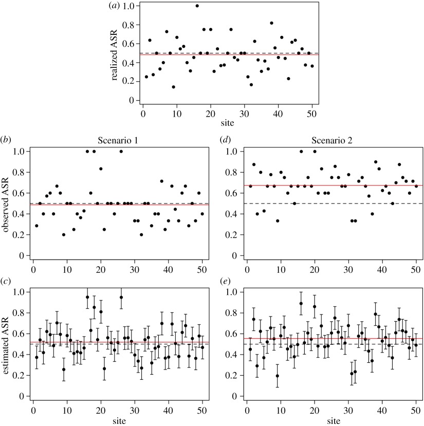
Box figure 1. Comparison of ASR measures from raw counts of unmarked male and female individuals with estimates obtained with a detection-based abundance model (the binomial-Poisson N-mixture model [80] as described above in the box. (a) The realized ASR for each site; (b,d) show the observed ASR obtained from raw counts for Scenarios 1 and 2, respectively; and (c,e) show ASR estimates generated with the binomial-Poisson N-mixture model that accounts for imperfect detection, with 95% confidence limits based on Monte Carlo sampling (see text). In all plots, red lines show mean values and dashed lines indicate the true ASR (0.5). Simulations were prepared in R [84] and models were constructed using the ‘pcount’ function of package ‘unmarked’ [85] (electronic supplementary material, appendix S1). (Online version in colour.)

Naturally, estimating ASRs from unmarked individuals requires that observed individuals be identified as males or females, which is not always possible. A possible method to handle uncertain observations where some individuals are classified as ‘sex not identified’ is an extension of the N-mixture model for estimating abundance when the identity of a species is uncertain [86]. The abundance model with species uncertainty estimates the probability of correctly assigning species' identity, in addition to site-specific abundance and detection probabilities. Description of the model structure is extensive, so we refer readers to the original article for details [86]. The model could be adapted for counts of males and females of a single species that also include individuals assigned to a ‘sex not identified’ category. Then, it would provide unbiased estimates of abundance for each sex, which can then be used to calculate the ASR as described above.

Although count surveys of unmarked individuals are generally simpler and require less effort than capture–mark–recapture surveys discussed in the next section, detection-based models usually require large sample sizes to parametrize. Because counts have to be divided between sexes, an even larger overall sample may be necessary to increase the precision of sex ratio estimates. Several methods, including most N-mixture models, require temporally replicated surveys and assume population closure (with respect to migration, births and deaths) throughout the study. Yet, many studies are based on multiple-season datasets with a single visit per season (e.g. the North American Breeding Bird Survey [87]), where the closure assumption is invalid [81]. Generalized multi-season abundance models [81,88,89] allow researchers to formally test the closure assumption through estimation of parameters of population dynamics, such as survival probability and recruitment rate [81], or population growth rate [88,89], and therefore, the model can be used to analyse count data when the closure assumption is invalid.

Although the approaches discussed in this section can generate estimates less biased than those derived from raw counts (box 1), we are not aware of any empirical study that has used any of these detection-based methods of estimating the ASR from unmarked individuals. We encourage researchers to use this type of procedure instead of simple counts whenever possible, because situations are very rare that allow every individual to be detected 100% of the time when direct counts are made, even for large diurnal mammals (e.g. [90–92]) and, surprisingly, for plants (e.g. [93,94]).

5. Detection-based methods of estimating the adult sex ratio from marked individuals

Observing individually marked or identifiable individuals characterizes many studies of animal behaviour and population biology. When estimating the ASR from counts of marked individuals, it is straightforward to account for detectability or catchability differences between the sexes by accounting for the sex-specific detection probabilities estimated from mark–recapture models, such as Cormack–Jolly–Seber models or multi-state capture–recapture models [2,95]. They use encounters (resightings and/or recaptures) of individually identifiable organisms, either tagged or recognizable by natural marks or scars (e.g. fin shapes, spot patterns), to generate robust estimates of resighting and demographic rates [96]. Mark–recapture models can be fitted for each sex to estimate sex-specific detection (p), survival rates, recruitment rates and population sizes (sex-specific abundances). Estimated sex-specific population sizes (N) can be further used to obtain an estimate of the ASR:

A few studies in wild populations of green-rumped parrotlets Forpus passerinus [2], common frogs [42] and Trinidadian guppies Poecilia reticulata [97] permit assessments of the robustness of this estimate (table 1), which could have broader applications for animal populations. Figure 3 illustrates annual estimates of sex ratio for two populations of parrotlets (one from a lowland site and the other from an upland site) derived from two methods. Differences (d) between the parrotlet ASR derived from the mark–recapture estimator (bars) and derived from raw counts of marked individuals (line) were small for most years (−0.05 ≤ d ≤ 0.05 for 20 of 30 annual estimates), but sizeable in other years (−0.1 ≥ d ≥ 0.1 for five of 30 annual estimates). There was a significant correlation between d and the resighting rates (p) of non-breeding males (NBM) and non-breeding females (NBF) (r = 0.69, p < 0.001), which are much more difficult to observe (mean ± s.e. for p_NBM = 0.58 + 0.04 and p_NBF = 0.43 + 0.05, n = 30) than breeding parrotlets (p = 1 for both sexes). Non-breeding males were significantly more likely to be resighted than non-breeding females (paired t-test, t = 2.69, d.f. = 29, p = 0.012), although detection probabilities varied greatly among years (p_NBM: 0.13–1.0; p_NBF: 0.05–1.0). Even when accounting for the lower detectability of non-breeding females, parrotlets exhibited male-biased sex ratios in all but 3 years. The large deviation from this pattern in 1992 in the upland population was caused by an extremely low resighting estimate for non-breeding females (p_female = 0.05), and suggests there will be situations where the mark–recapture estimator of sex ratio may not perform well [2].

Table 1.

Examples of the use of different approaches for estimating ASR that account for detection differences between the sexes or reconstruct the ASR from sex-specific demographic rates. The vast majority of ASR estimates come from raw counts of unmarked individuals, alive or dead, and do not correct for potential biases associated with sex difference in detectability or catchability (e.g. amphibians, birds, mammals and reptiles [98]; fish [99]; crustaceans [76,100]; insects [101]).

ASR estimation method	group	species	source
detection-based estimates from unmarked individuals	none	—	—
detection-based estimates from marked individuals	amphibians	common frog Rana temporaria	Alho et al. [42]
	birds	green-rumped parrotlet Forpus passerinus	Veran & Beissinger [2]
		willow warbler Phylloscopus trochilus	Morrison et al. [102]
	fish	trinidadian guppy Poecilia reticulata	Arendt et al. [97]
	mammals	roosevelt elk Cervus elaphus roosevelti	Weaver & Weckerly [103]
indirect estimators	birds	snowy plover Charadrius nivosus	Warriner et al. [104]
		Kentish plover Charadrius alexandrinus	Kosztolányi et al. [105]
		green-rumped parrotlet	Veran & Beissinger [2]
	mammals	Norwegian moose Alces alces	Solberg et al. [12]
		white-tailed deer Odocoileus virginianus	Severinghaus & Maguire [106]

Figure 3.

Comparison of ASRs (males/(males + females)) of green-rumped parrotlets estimated by counts of the number of breeding and non-breeding adults of each sex resighted annually (line) and after correcting for detection probability by dividing each count by the annual sex- and stage-specific (non-breeder and breeder) probability of detection (bars) for the upland population (a) and lowland population (b). Adapted from Veran & Beissinger [2].

The past 25 years have seen the development of powerful statistical methods and software [107,108] for analysing a great diversity of mark–recapture data [96]. In general, mark–recapture models require that individuals be individually marked or identifiable, animals do not lose their marks and samples are temporally replicated. Moreover, the time span between capture occasions must be substantially longer than the duration of the capture events [109]. See Sandercock [110] for an outstanding review of the many approaches to structure mark–recapture models and their potential use for estimating demographic parameters that can be applied to modelling sex differences.

6. Indirect estimators of the adult sex ratio

Indirect methods for estimating the ASR do not directly sample the number of males and females counted or captured in a population, but instead estimate the ASR using relationships that emerge from measures of demography, such as survival, age structure, reproduction and assumed dynamics. Indirect measures of the ASR were initially developed for managing game species using harvest data or when one sex was not easily observed [111].

Sex ratios have been projected from sex-specific probabilities of survival using the ratio of the sum of the male survival divided by the sum of female survival for adult and/or subadult classes [111]. The method may be extended to incorporate information on juvenile sex ratios and natural and harvest mortality for males and females when data are available [104,111,112]. Estimates of the ASR based on survival probabilities can be adjusted for scenarios when survival is equal for all age classes, or differs between juveniles and various different adult stages [111]. Box 2 presents a detailed example for the Kentish plover (Charadrius alexandrinus).

Box 2. Demographic estimate of the adult sex ratio in the Kentish plover.

A small shorebird, the Kentish plover C. alexandrinus (body mass 40–44 g) (box figure 2) is often used as an ecological model system to understand costs and benefits of mating systems and parental care because they exhibit diverse reproductive tactics [113–115]. They produce two to three eggs in a small scrape on the ground and both parents incubate the eggs, although after hatching of the eggs one of the parents usually abandons the brood and re-nests with a new mate. In several plover populations, more female than male parents abandon the young, and Székely & Lessells [114] hypothesized that female desertion is facilitated by a male-biased ASR.

Box figure 2. Female Kentish plover incubating the eggs (credit: Hugo Amador). (Online version in colour.)

To test this proposition, Kosztolányi et al. [105] used 5 years of data from an intensely monitored plover population in Southern Turkey. Using data from 2101 individuals, including 579 molecularly sexed offspring, and by estimating nest survival and sex-specific survival of juveniles and adults and running the model through all age cohorts (box figure 3), the model showed that males outnumber females in the population (ASR = 0.860, 0.791–0.904 (95% confidence intervals)). The strong male bias was robust because it remained consistent when one year was excluded from the dataset (box figure 4).

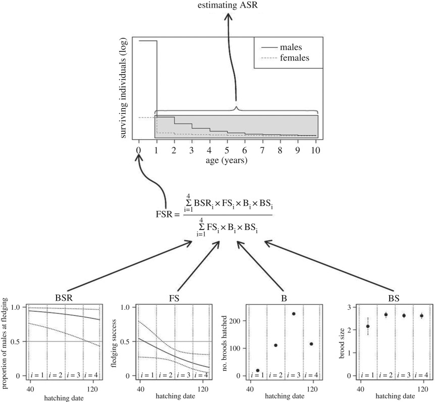
Box figure 3. Schematic view of the demographic model used to estimate the ASR in the Kentish plover (BSR, brood sex ratio; FS, fledging success; B, number of broods that hatch; BS, brood size; FSR, fledgling sex ratio; [105]).

The result of Kosztolányi et al. [105] is consistent with two additional lines of evidence. First, when the mating opportunities of male and female Kentish plovers were estimated experimentally by removing the mate, the remating probability of females was five to eight times higher than that of males [116]; this difference is consistent with the magnitude of the bias in the ASR estimated by demographic modelling (6.1 times more males than females; [105]). Note that the demography-based ASR is not entirely equivalent to the experimentally estimated mating opportunities because the latter is a derivative of the OSR [117]. Second, a recent two stage two sex model using the approach of Veran & Beissinger [2] estimated the stable ASR distribution of the same plover population to ASR = 0.59 (0.51–0.65, 95% CI)—a significantly male-biased ASR but somehow less extreme than Kosztolányi et al.'s estimate (LJ Eberhart-Phillips et al. 2017, unpublished data).

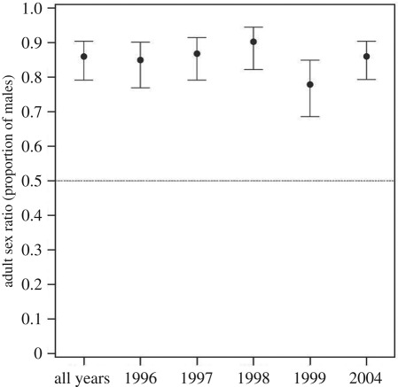
Box figure 4. The adult sex ratio (ASR, mean ± 95% confidence limits proportion of males) in the Kentish plover based on 5 years and by excluding a given year from the dataset [105].

Age structure inferred from sex-biased harvest data has been used in combination with survival data to derive the sex ratio of a harvested adult population. This approach was first developed by Severinghaus & Maguire [106] for estimating the juvenile sex ratio from hunter kills of deer as the proportion of yearling to adult males divided by the proportion of yearling to adult females. Derivations of this approach have been developed with differing assumptions about demographic rates for the juvenile age class: juvenile survival is equal for males and females, juvenile survival differs between sexes, juvenile sex ratios do not differ from unity and juvenile sex ratios are unequal [111]. Nevertheless, this method and its derivations rely deeply on three assumptions that are often not met in the focal population: harvest probabilities of different age classes are equal, age structure remains constant over time and recruitment rates do not differ between males and females.

If sufficient data are available to estimate sex-specific demography for the entire life cycle of an organism, the male and female proportions of a population can be calculated directly from two-sex matrix population models [2,95,118]. Matrix population models are numerical representations of the life cycle of an organism [119]. Single-sex matrix population models, usually female-based, are commonly used to estimate the asymptotic growth rate (λ) of a population as well as its sensitivity or elasticity, which measure the impact of change in a demographic rate (e.g. survival, growth or reproduction) on λ [120]. In these discrete-time models, nodes denote distinct life-history stages that experience different demographic rates, and the transition between nodes/stages is conditioned on parameters representing key demographic processes (see [119,121] for reviews). The stable (st)age distribution, which is the proportion of individuals in each (st)age class, is an emergent property if the rates of survival, growth and reproduction remain constant from year to year.

The two-sex formulation of a matrix model allows demographic rates to differ between males and females on the basis of empirical observations. Estimates of demographic parameters of interest are used to parametrize matrix elements separately for each sex, and they are linked by a mating and birth function that incorporates the demographic interactions between the sexes. The ASR can be deduced from the model based on proportions of the stable-stage distribution of males and females for the appropriate nodes of interest ([2]; figure 4). In addition, metrics of sensitivity developed by Veran & Beissinger [2] and applied to the stable-stage distribution instead of λ can be used to diagnose potential causes of biased sex ratios by quantifying which demographic parameters contribute most to an unbalanced ASR. For example, despite a sizeable difference in adult survival between green-rumped parrotlet sexes, this rate contributed much less to the skewed ASR than the low rate of female juvenile local survival and philopatry caused by sex-biased dispersal [2].

Figure 4.

(a) Life cycle diagram composed of four stages (NBF, non-breeding females; BF, breeding females; NBM, non-breeding males; BM, breeding males) for green-rumped parrotlets based on pre-breeding censuses. (b) Projection matrix used to deduce the ASR from the model based on proportions of the stable-stage distribution of males and females in the appropriate nodes of interest [2]. Notation includes: ϕ, probability of local survival; ψ, probability of becoming or remaining a breeder; R, fecundity; ρ, primary sex-ratio; I, immigration rate. Subscripts include: JF, juvenile females; JM, juvenile males. Adapted from Veran & Beissinger [2].

While indirect estimators can answer questions about the origin of ASR difference that other methods cannot address, two-sex matrix models require extensive data to parametrize and, if such data exist, it seems likely that it often would be possible to obtain the direct measures of sex ratio discussed in previous sections. Nevertheless, there may be situations where direct estimates of sex ratio do not exist, but data are available to parametrize a two-sex matrix model [122].

The indirect methods discussed in this section assume that model parameters (e.g. annual recruitment, age-specific growth and survival, and harvest rates) remain more or less constant over time because they estimate sex ratios from stable (st)age distributions. This assumption will be violated in nature to varying degrees, so indirect estimations of the ASR should be considered as hypothesized sex ratios rather than actual estimations of the ASR. Nevertheless, these approaches have value, as they can be used to assess the impacts of alternative management scenarios on age- or sex-structure of a population [111], or to make ecological or evolutionary inferences [2].

7. Discussion

Understanding the causes and implications of ASR variation is essential for the study of population dynamics, the evolution of social behaviour and sexual selection in humans and most animals [3,5,9,12], and the ASR provides important insights for management of species of high conservation concern or commercial importance [16,17]. However, to advance this field, more accurate and comparable ASR estimates are needed across a wide range of species [4,101].

Our review has five main recommendations. First, we suggest that the proportion of males in the adult population (i.e. ASR = N_male/(N_male + N_female)) is the best general measure to quantify the ASR. It takes on easily interpreted values between 0 and 1 that reflect the relative abundances of males and females in the adult population. Although the ASR is traditionally expressed as ratios of one sex to the other (e.g. M : F), these have unfavourable properties because they have an upper boundary of infinity and tend to be asymmetric.

Second, we think it is useful to expand the established sex ratios to incorporate additional life-history stages. In addition to the well-established terminology of primary, secondary, tertiary, operational and quaternary sex ratios, we also recognize two additional terms: juvenile sex ratios and MSR. Researchers need to bear in mind that some of these represent sex ratios at a given time (i.e. fertilization, birth, maturation), whereas others integrate over a number of age cohorts (e.g. juvenile sex ratio, ASR). Although some of these sex ratios have been intensely investigated in selected organisms, few studies aimed at establishing sex ratio variation across the entire lifespan of animals. As selective processes spill over to affect subsequent life stages (e.g. early developmental experiences may influence survival and reproduction later in life [123]), studies are needed that investigate causes and implications of sex ratio biases in an integrative way.

Third, sex differences in morphology, ecology and behaviour are common in nature and are expected to result in sex differences in detectability or catchability, and therefore, could bias ASR estimates [17,31,34]. It is necessary to assess the extent to which ASR estimates can be affected by differences in the probability of detecting or catching males and females in wild animal populations [33,34]. We have also highlighted that ASR estimates can be further biased if non-breeding adults are missed from sampling due to their less conspicuous lifestyles [36,37]. As the vast majority of current ASR estimates have been derived using methods that do not correct for these potential biases [17,98,124] (table 1), we encourage researchers to use mark–recapture models or other detection-based methods for unmarked individuals that control for the sources of some of these biases. Nonetheless, we caution against throwing the baby out with the bathwater, given that at least in one taxon, the birds, the published ASR estimates have high intra-class correlation (figure 2).

Efforts to study ASRs of unmarked populations may benefit from the integration of methods that estimate the probability of correct sexual identification (i.e. adapting [86] to a single-species dataset of male and female counts) and those that estimate demographic parameters from counts (e.g. survival [81]). This integrative approach would allow estimation of the abundance of each sex, sex-specific survival rates and the ASR while accounting for uncertainty in sexual identification in vertebrate and invertebrate populations.

Fourth, while mark–recapture-based estimates of ASRs correct for sources of detectability, they sometimes have their own problems. Being captured in a given year could affect the probability of skipping reproduction in the next year and, depending on the sex of adults, could affect ASR estimates [42,96]. Also, mark–recapture methods require large numbers of marked individuals for reliable estimates. Sex differences in dispersal can distort recapture probability estimates, because permanent emigration can rarely be distinguished from death. Nevertheless, mark–recapture models for marked populations and detection-based methods for unmarked populations should be used for estimating the ASR, and combined with estimation of sex-specific immigration and emigration rates. With increased use of GPS tags and movement monitoring devices, researchers will be able to quantify sex-specific differences in dispersal, activity patterns and other behavioural factors, which should increase our understanding of the sources of sex differences in detectability and, in turn, sex ratio variation.

In addition to intrinsic factors that lead to sex differences in detectability or catchability, attention must be paid to the choice of sampling or trapping methods, as bait-based sampling or trapping techniques can have selective effects on males and females, and thus, could give rise to systematic distortions in ASR estimates [57,74,76]. A possible solution to this problem could be using spatially and temporally stratified sampling (or trapping) techniques for a given population. As a general recommendation, ASR estimates based on hunting bags should be avoided, because they are admittedly biased by sex and potentially by age due to hunting restrictions and hunter preferences [111].

Fifth, the ASR is a population parameter that may vary considerably in space and time [50,102], and this variation has been noted by wildlife biologists for half a century [125,126]. Thus, obtaining reliable ASR estimates requires choosing an appropriate spatial scale and, in most cases, carrying out long-term sampling programmes [101]. Studies examining the causes and consequences of spatial and temporal variation in the ASR at the local and regional (i.e. metapopulation) scale are rare [102], but they are urgently needed for (at least) three reasons. First, in migratory species, estimating the ASR at stopover sites may not reflect the sex ratio of a population as a whole, but only sexual differences in migratory patterns [71]. Second, the ASR may be balanced at a metapopulation scale even when it is locally biased towards one specific sex [127]. And third, ASR estimates may depend on variation in activity patterns [33,42].

8. Conclusion

Obtaining robust ASR estimates of wild animal populations can be challenging, but current statistical advances offer plausible solutions to major difficulties stemming from the effects of spatial and temporal variation in the numbers of males and females, and detection or capture probabilities that differ between the sexes. We recommend that detection-based methods be useful for estimating ASR in most situations, and point out that studies are needed to establish the consistency between ASR estimates obtained by different estimation methods [31] and control for sex differences in dispersal. These advances will be key to draw proper inferences about the fascinating ecological and evolutionary implications of ASR variation for human and non-human societies. They can also contribute to wildlife conservation, because accurate ASR estimates may be important when assessing viability of animal populations (e.g. reptiles, fish, mammals and birds; reviewed in [17]) and can lead to better management policies [17,22,23].

Data accessibility

This article has no additional data.

Authors' contributions

S.A., T.S. and S.R.B. conceived and designed the study; S.A., F.V.D., T.S. and S.R.B. collected the data, performed the analyses and wrote the manuscript. All authors contributed critically to the drafts and gave final approval for publication.

Competing interests

We declare we have no competing interests.

Funding

S.A. was supported by CONACYT (Mexico). T.S. was supported by Hungarian Science Foundation (NKFIH-K116310). T.S. and S.R.B. were supported as Fellows at the Wissenschaftskolleg zu Berlin during the production of this contribution.

References

- 1.Wilson EO. 1975. Sociobiology: the new synthesis. Cambridge, MA: Harvard University Press. [Google Scholar]
- 2.Veran S, Beissinger SR. 2009. Demographic origins of skewed operational and adult sex ratios: perturbation analyses of two-sex models. Ecol. Lett. 12, 129–143. ( 10.1111/j.1461-0248.2008.01268.x) [DOI] [PubMed] [Google Scholar]
- 3.McNamara JM, Székely T, Webb JN, Houston AI. 2000. A dynamic game-theoretic model of parental care. J. Theor. Biol. 205, 605–623. ( 10.1006/jtbi.2000.2093) [DOI] [PubMed] [Google Scholar]
- 4.Székely T, Weissing FJ, Komdeur J. 2014. Adult sex ratio variation: implications for breeding system evolution. J. Evol. Biol. 27, 1500–1512. ( 10.1111/jeb.12415) [DOI] [PubMed] [Google Scholar]
- 5.Kokko H, Jennions MD. 2008. Parental investment, sexual selection and sex ratios. J. Evol. Biol. 21, 919–948. ( 10.1111/j.1420-9101.2008.01540.x) [DOI] [PubMed] [Google Scholar]
- 6.Clutton-Brock TH, Coulson TN, Milner-Gulland EJ, Thomson D, Armstrong HM. 2002. Sex differences in emigration and mortality affect optimal management of deer populations. Nature 415, 633–637. ( 10.1038/415633a) [DOI] [PubMed] [Google Scholar]
- 7.Dyson EA, Hurst GDD. 2004. Persistence of an extreme sex-ratio bias in a natural population. Proc. Natl Acad. Sci. USA 101, 6520–6523. ( 10.1073/pnas.0304068101) [DOI] [PMC free article] [PubMed] [Google Scholar]
- 8.Pettersson LB, Ramnarine IW, Becher SA, Mahabir R, Magurran AE. 2004. Sex ratio dynamics and fluctuating selection pressures in natural populations of the Trinidadian guppy, Poecilia reticulata. Behav. Ecol. Sociobiol. 55, 461–468. ( 10.1007/s00265-003-0727-8) [DOI] [Google Scholar]
- 9.Le Galliard JF, Fitze PS, Ferrière R, Clobert J. 2005. Sex ratio bias, male aggression, and population collapse in lizards. Proc. Natl Acad. Sci. USA 102, 18 231–18 236. ( 10.1073/pnas.0505172102) [DOI] [PMC free article] [PubMed] [Google Scholar]
- 10.Liker A, Székely T. 2005. Mortality costs of sexual selection and parental care in natural populations of birds. Evolution 59, 890–897. ( 10.1554/04-560) [DOI] [PubMed] [Google Scholar]
- 11.Clutton-Brock T. 1991. The evolution of parental care. Princeton, NJ: Princeton University Press. [Google Scholar]
- 12.Solberg EJ, Loison A, Ringsby TH, Sæther B-E, Heim M. 2002. Biased adult sex ratio can affect fecundity in primiparous moose Alces alces. Wildl. Biol. 8, 117–128. [Google Scholar]
- 13.Brooke MD, Flower TP, Mainwaring MC. 2010. A scarcity of females may constrain population growth of threatened bird species: case notes from the critically endangered Raso lark Alauda razae. Bird Conserv. Int. 20, 382–384. ( 10.1017/S0959270910000225) [DOI] [Google Scholar]
- 14.Hovestadt T, Mitesser O, Poethke H-J. 2014. Gender-specific emigration decisions sensitive to local male and female density. Am. Nat. 184, 38–51. ( 10.1086/676524) [DOI] [PubMed] [Google Scholar]
- 15.Bessa-Gomes C, Legendre S, Clobert J. 2004. Allee effects, mating systems and the extinction risk in populations with two sexes. Ecol. Lett. 7, 802–812. ( 10.1111/j.1461-0248.2004.00632.x) [DOI] [Google Scholar]
- 16.Lee AM, Saether B-E, Engen S. 2011. Demographic stochasticity, Allee effects, and extinction: the influence of mating system and sex ratio. Am. Nat. 177, 301–313. ( 10.1086/658344) [DOI] [PubMed] [Google Scholar]
- 17.Donald PF. 2007. Adult sex ratios in wild bird populations. Ibis (Lond. 1859) 149, 671–692. ( 10.1111/j.1474-919X.2007.00724.x) [DOI] [Google Scholar]
- 18.Byrne PG, Roberts JD. 1999. Simultaneous mating with multiple mates reduces fertilization success in the myobatrachid frog Crinia georgiana. Proc. R. Soc. Lond. B 266, 717–721. ( 10.1098/rspb.1999.0695) [DOI] [Google Scholar]
- 19.Banks SC, Hoyle SD, Horsup A, Sunnucks P, Taylor AC. 2003. Demographic monitoring of an entire species (the northern hairy-nosed wombat, Lasiorhinus krefftii) by genetic analysis of non-invasively collected material. Anim. Conserv. 6, 101–107. ( 10.1017/S1367943002004000) [DOI] [Google Scholar]
- 20.Marsden JEE, Robillard SR. 2004. Decline of yellow perch in southwestern Lake Michigan, 1987–1997. North Am. J. Fish. Manag. 24, 952–966. ( 10.1577/M02-195.1) [DOI] [Google Scholar]
- 21.Charlat S, Reuter M, Dyson EA, Hornett EA, Duplouy A, Davies N, Roderick GK, Wedell N, Hurst GD. 2007. Male-killing bacteria trigger a cycle of increasing male fatigue and female promiscuity. Curr. Biol. 17, 273–277. ( 10.1016/j.cub.2006.11.068) [DOI] [PubMed] [Google Scholar]
- 22.Hoffman JD, Genoways HH. 2012. Examination of annual variation in the adult sex ratio of pronghorn (Antilocapra americana). Am. Midl. Nat. 168, 289–301. ( 10.1674/0003-0031-168.2.289) [DOI] [Google Scholar]
- 23.de Martini EE, Everson AR, Nichols RS. 2011. Estimates of body sizes at maturation and at sex change, and the spawning seasonality and sex ratio of the endemic Hawaiian grouper (Hyporthodus quernus F. Epinephelidae). Fish. Bull. 109, 123–134. [Google Scholar]
- 24.Trent K, South SJ. 2011. Too many men? Sex ratios and women's partnering behavior in China. Soc. Forces 90, 247–267. ( 10.1093/sf/90.1.247) [DOI] [PMC free article] [PubMed] [Google Scholar]
- 25.Griskevicius V, Tybur JM, Ackerman JM, Delton AW, Robertson TE, White AE. 2012. The financial consequences of too many men: sex ratio effects on saving, borrowing, and spending. J. Pers. Soc. Psychol. 102, 69–80. ( 10.1037/a0024761) [DOI] [PMC free article] [PubMed] [Google Scholar]
- 26.Schacht R, Rauch KL, Borgerhoff-Mulder M. 2014. Too many men: the violence problem? Trends Ecol. Evol. 29, 214–221. ( 10.1016/j.tree.2014.02.001) [DOI] [PubMed] [Google Scholar]
- 27.Hesketh T, Xing ZW. 2006. Abnormal sex ratios in human populations: causes and consequences. Proc. Natl. Acad. Sci. USA 103, 13 271–13 275. ( 10.1073/pnas.0602203103) [DOI] [PMC free article] [PubMed] [Google Scholar]
- 28.Census 2000. Accuracy and coverage evaluation of census 2000: design and methodology. U.S. Census Bureau, 2004. Available online at https://www.census.gov/prod/2004pubs/dssd03-dm.pdf.
- 29.Guillot M. 2002. The dynamics of the population sex ratio in India, 1971–96. Popul. Stud. 56, 51–63. ( 10.1080/00324720213795) [DOI] [PubMed] [Google Scholar]
- 30.Baumgardt JA, Goldberg CS, Reese KP, Connelly JW, Musil DD, Garton EO, Waits LP. 2013. A method for estimating population sex ratio for sage-grouse using noninvasive genetic samples. Mol. Ecol. Resour. 13, 393–402. ( 10.1111/1755-0998.12069) [DOI] [PubMed] [Google Scholar]
- 31.Weaver S, Weckerly F. 2011. Sex ratio estimates of Roosevelt elk using counts and Bowden's estimator. Calif. Fish Game 97, 130–137. [Google Scholar]
- 32.Vanderkist BA, Xue XH, Griffiths R, Martin K, Beauchamp WD, Williams TD. 1999. Evidence of male-bias in capture samples of marbled murrelets from genetic studies in British Columbia. Condor 101, 398–402. ( 10.2307/1370004) [DOI] [Google Scholar]
- 33.Pickett EJ, Stockwell MP, Pollard CJ, Garnham JI, Clulow J, Mahony MJ. 2012. Estimates of sex ratio require the incorporation of unequal catchability between sexes. Wildl. Res. 39, 350–354. ( 10.1071/WR11193) [DOI] [Google Scholar]
- 34.Amrhein V, Scaar B, Baumann M, Minéry N, Binnert JP, Korner-Nievergelt F. 2012. Estimating adult sex ratios from bird mist netting data. Methods Ecol. Evol. 3, 713–720. ( 10.1111/j.2041-210X.2012.00207.x) [DOI] [Google Scholar]
- 35.Rodrigues JF. M., Coelho MTP, Wirsing A, Dill L, Gaston K, Münkemüller T. 2016. Differences in movement pattern and detectability between males and females influence how common sampling methods estimate sex ratio. PLoS ONE 11, e0159736 ( 10.1371/journal.pone.0159736) [DOI] [PMC free article] [PubMed] [Google Scholar]
- 36.Nichols JD, Hines JE, Pollock KH, Hinz RL, Link WA. 1994. Estimating breeding proportions and testing hypotheses about costs of reproduction with capture–recapture data. Ecology 75, 2052–2065. ( 10.2307/1941610) [DOI] [Google Scholar]
- 37.Lee AM, Reid JM, Beissinger SR. 2017. Modeling effects of nonbreeders on population growth estimates. J. Anim. Ecol. 86, 75–87. ( 10.1111/1365-2656.12592) [DOI] [PubMed] [Google Scholar]
- 38.Le Boeuf BJ, Peterson RS. 1969. Social status and mating activity in elephant seals. Science 163, 91–93. ( 10.1126/science.163.3862.91) [DOI] [PubMed] [Google Scholar]
- 39.Ruckstuhl KE, Neuhaus P. 2005. Sexual segregation in vertebrates: ecology of the two sexes. Cambridge, UK: Cambridge University Press. [Google Scholar]
- 40.Heithaus MR, Hamilton IM, Wirsing AJ, Dill LM. 2006. Validation of a randomization procedure to assess animal habitat preferences: microhabitat use of tiger sharks in a seagrass ecosystem. J. Anim. Ecol. 75, 666–676. ( 10.1111/j.1365-2656.2006.01087.x) [DOI] [PubMed] [Google Scholar]
- 41.Joron M. 2005. Polymorphic mimicry, microhabitat use, and sex-specific behaviour. J. Evol. Biol. 18, 547–556. ( 10.1111/j.1420-9101.2005.00880.x) [DOI] [PubMed] [Google Scholar]
- 42.Alho JS, Herczeg G, Merilä J. 2008. Female-biased sex ratios in subarctic common frogs. J. Zool. 275, 57–63. ( 10.1111/j.1469-7998.2007.00409.x) [DOI] [Google Scholar]
- 43.Jaatinen K, Lehikoinen A, Lank DB. 2010. Female-biased sex ratios and the proportion of cryptic male morphs of migrant juvenile Ruffs (Philomachus pugnax) in Finland. Ornis Fenn. 87, 125–134. [Google Scholar]
- 44.Schärer L, Janicke T, Ramm SA. 2015. Sexual conflict in hermaphrodites. Cold Spring Harb. Perspect. Biol. 7, a017673 ( 10.1101/cshperspect.a017673) [DOI] [PMC free article] [PubMed] [Google Scholar]
- 45.Pickup M, Barrett SC. H. 2013. The influence of demography and local mating environment on sex ratios in a wind-pollinated dioecious plant. Ecol. Evol. 3, 629–639. ( 10.1002/ece3.465) [DOI] [PMC free article] [PubMed] [Google Scholar]
- 46.Field DL, Pickup M, Barrett SCH. 2013. Comparative analyses of sex-ratio variation in dioecious flowering plants. Evolution 67, 661–672. ( 10.1111/evo.12001) [DOI] [PubMed] [Google Scholar]
- 47.Taylor DR. 1999. Genetics of sex ratio variation among natural populations of a dioecious plant. Evolution 53, 55 ( 10.2307/2640919) [DOI] [PubMed] [Google Scholar]
- 48.Wilson K, Hardy ICW. 2002. Statistical analysis of sex ratios: an introduction. In Sex ratios: concepts and research methods (ed. ICW Hardy), pp. 46–92. Cambridge, UK: Cambridge University Press. [Google Scholar]
- 49.Emlen S, Oring L. 1977. Ecology, sexual selection, and the evolution of mating systems. Science 197, 215–223. ( 10.1126/science.327542) [DOI] [PubMed] [Google Scholar]
- 50.Carmona-Isunza M, Ancona S, Székely T, Ramallo-González A, Cruz-López M, Serrano-Meneses MA, Küpper C. 2017. Adult sex ratio and operational sex ratio exhibit different temporal dynamics in the wild. Behav. Ecol. 28, 523–532. ( 10.1093/beheco/arw183) [DOI] [Google Scholar]
- 51.Székely T, Webb JN, Cuthill I. 2000. Mating patterns, sexual selection and parental care: an integrative approach. In Vertebrate mating systems (eds Apollonio M, Festa-Bianchet M, Mainardi D), pp. 194–223. London, UK: World Science Press. [Google Scholar]
- 52.Kramer KL, Schacht R, Bell A. 2017. Adult sex ratios and partner scarcity among hunter–gatherers: implications for dispersal patterns and the evolution of human sociality. Phil. Trans. R. Soc. B 372, 20160316 ( 10.1098/rstb.2016.0316) [DOI] [PMC free article] [PubMed] [Google Scholar]
- 53.Croft DP, Brent LJ. N., Franks DW, Cant MA. 2015. The evolution of prolonged life after reproduction. Trends Ecol. Evol. 30, 407–416. ( 10.1016/j.tree.2015.04.011) [DOI] [PubMed] [Google Scholar]
- 54.Fairbairn DJ. 2007. Introduction: the enigma of sexual size dimorphism. In Sex, size and gender roles (eds Fairbairn DJ, Blanckenhorn WU, Székely T), pp. 1–10. Oxford, UK: Oxford University Press. [Google Scholar]
- 55.Ranta E, Laurila A, Elmberg J. 1994. Reinventing the wheel: analysis of sexual dimorphism in body size. Oikos 70, 313–321. ( 10.2307/3545768) [DOI] [Google Scholar]
- 56.Frey DF, Leong KL. H. 1993. Can microhabitat selection or differences in ‘catchability’ explain male-biased sex ratios in overwintering populations of monarch butterflies? Anim. Behav. 45, 1025–1027. ( 10.1006/anbe.1993.1120) [DOI] [Google Scholar]
- 57.Domènech J, Senar JC. 1998. Trap type can bias estimates of sex ratio. J. F. Ornithol. 69, 380–385. [Google Scholar]
- 58.McCullough DR, Weckerly FW, Garcia PI, Evett RR. 1994. Sources of inaccuracy in black-tailed deer herd composition counts. J. Wildl. Manage. 58, 319–329. ( 10.2307/3809397) [DOI] [Google Scholar]
- 59.Marealle WN, Fossøy F, Holmern T, Stokke BG, Røskaft E. 2010. Does illegal hunting skew Serengeti wildlife sex ratios? Wildlife Biol. 16, 419–429. ( 10.2981/10-035) [DOI] [Google Scholar]
- 60.Berger J, Gompper M. 1999. Sex ratios in extant ungulates: products of contemporary predation or past life histories? J. Mammal. 80, 1084–1113. ( 10.2307/1383162) [DOI] [Google Scholar]
- 61.Adler GH, Lambert TD. 1997. Ecological correlates of trap response of a Neotropical forest rodent, Proechimys semispinosus. J. Trop. Ecol. 13, 59–68. ( 10.1017/S0266467400010257) [DOI] [Google Scholar]
- 62.Götmark F, Hohlfält A. 1995. Bright male plumage and predation risk in passerine birds: are males easier to detect than females? Oikos 74, 475–484. ( 10.2307/3545993) [DOI] [Google Scholar]
- 63.Duarte A, Hines JE, Nichols JD, Hatfield JS, Weckerly FW. 2014. Age-specific survival of male golden-cheeked warblers on the Fort Hood military reservation, Texas. Avian Conserv. Ecol. 9, 4 ( 10.5751/ACE-00693-090204) [DOI] [Google Scholar]
- 64.Sandercock BK, Székely T, Kosztolányi A. 2005. The effects of age and sex on the apparent survival of Kentish plovers breeding in southern Turkey. Condor 107, 583 ( 10.1650/0010-5422(2005)107%5B0583:TEOAAS%5D2.0.CO;2) [DOI] [Google Scholar]
- 65.Andreassen HP, Bondrup-Nielsen S. 1991. Home range size and activity of the wood lemming, Myopus schisticolor. Ecography (Cop.) 14, 138–141. ( 10.1111/j.1600-0587.1991.tb00644.x) [DOI] [Google Scholar]
- 66.Drickamer LC, Lenington S, Erhart M, Robinson AS. 1994. Trappability of wild house mice (Mus domesticus) in large outdoor pens: implication for models of t-complex gene frequency. Am. Midl. Nat. 133, 283–289. ( 10.2307/2426392) [DOI] [Google Scholar]
- 67.Gehrt SD, Fritzell EK. 1997. Sexual differences in home ranges of raccoons. J. Mammal. 78, 921–931. ( 10.2307/1382952) [DOI] [Google Scholar]
- 68.Solmundsson J, Karlsson H, Palsson J. 2003. Sexual differences in spawning behaviour and catchability of plaice (Pleuronectes platessa) west of Iceland. Fish. Res. 61, 57–71. ( 10.1016/S0165-7836(02)00212-6) [DOI] [Google Scholar]
- 69.Payne NL, Gillanders BM, Semmens J. 2011. Breeding durations as estimators of adult sex ratios and population size. Oecologia 165, 341–347. ( 10.1007/s00442-010-1729-7) [DOI] [PubMed] [Google Scholar]
- 70.Davis AK, Rendón-Salinas E. 2010. Are female monarch butterflies declining in eastern North America? Evidence of a 30-year change in sex ratios at Mexican overwintering sites. Biol. Lett. 6, 45–47. ( 10.1098/rsbl.2009.0632) [DOI] [PMC free article] [PubMed] [Google Scholar]
- 71.Lebret T. 1950. The sex-ratios and the proportion of adult drakes of teal, pintail, shoveler and wigeon in the Netherlands, based on field counts made during autumn, winter and spring. Ardea 38, 1–18. [Google Scholar]
- 72.White GC, Freddy DJ, Gill RB, Ellenberger JH. 2001. Effect of adult sex ratio on mule deer and elk productivity in Colorado. J. Wildl. Manage. 65, 543–551. ( 10.2307/3803107) [DOI] [Google Scholar]
- 73.Bull JJ, Shine R. 1979. Iteroparous animals that skip opportunities for reproduction. Am. Nat. 114, 296–303. ( 10.1086/283476) [DOI] [Google Scholar]
- 74.Henderson PA, Southwood R. 2016. Ecological methods, 4th edn Chichester, West Sussex: John Wiley & Sons, Inc. [Google Scholar]
- 75.Southwood TR. E. 1960. The flight activity of Heteroptera. Trans. R. Entomol. Soc. Lond. 112, 173–220. ( 10.1111/j.1365-2311.1960.tb00498.x) [DOI] [Google Scholar]
- 76.Johnson P. 2003. Biased sex ratios in fiddler crabs (Brachyura, Ocypodidae): a review and evaluation of the influence of sampling method, size class, and sex-specific mortality. Crustaceana 76, 559–580. ( 10.1163/156854003322316209) [DOI] [Google Scholar]
- 77.Agnello AM, Reissig WH, Spangler SM, Charlton RE, Kain DP. 1996. Trap response and fruit damage by obliquebanded leafroller (Lepidoptera: Tortricideae) in pheromone-treated apple orchards in New York. Environ. Entomol. 25, 268–282. ( 10.1093/ee/25.2.268) [DOI] [Google Scholar]
- 78.Dénes FV, Silveira LF, Beissinger SR. 2015. Estimating abundance of unmarked animal populations: accounting for imperfect detection and other sources of zero inflation. Methods Ecol. Evol. 6, 543–556. ( 10.1111/2041-210X.12333) [DOI] [Google Scholar]
- 79.Kéry M, Royle JA. 2016. Applied hierarchical modeling in ecology. Amsterdam, The Netherlands: Elsevier. [Google Scholar]
- 80.Royle JA. 2004. N-mixture models for estimating population size from spatially replicated counts. Biometrics 60, 108–115. ( 10.1111/j.0006-341X.2004.00142.x) [DOI] [PubMed] [Google Scholar]
- 81.Dail D, Madsen L. 2011. Models for estimating abundance from repeated counts of an open metapopulation. Biometrics 67, 577–587. ( 10.1111/j.1541-0420.2010.01465.x) [DOI] [PubMed] [Google Scholar]
- 82.Buckland S, Anderson D, Burnham KP, Laake JL, Borchers DL, Thomas L. 2001. Introduction to distance sampling: estimating abundance of biological populations. Oxford, UK: Oxford University Press. [Google Scholar]
- 83.Sólymos P, Lele S, Bayne E. 2012. Conditional likelihood approach for analyzing single visit abundance survey data in the presence of zero inflation and detection error. Environmetrics 23, 197–205. ( 10.1002/env.1149) [DOI] [Google Scholar]
- 84.R Development Core Team. 2016. R: a language and environment for statistical computing. R Foundation for Statistical Computing, Vienna, Austria. http://www.Rproject.org/.
- 85.Fiske I, Chandler R. 2011. Unmarked: an R package for fitting hierarchical models of wildlife occurrence and abundance. J. Stat. Softw. 43, 1–23. ( 10.18637/jss.v043.i10) [DOI] [Google Scholar]
- 86.Chambert T, Hossack BR, Fishback L, Davenport JM. 2016. Estimating abundance in the presence of species uncertainty. Methods Ecol. Evol. 7, 1041–1049. ( 10.1111/2041-210X.12570) [DOI] [Google Scholar]
- 87.Robbins CS, Bystrak D, Geissler PH. 1986. The breeding bird survey: its first fifteen years, 1965–1979. Washington, DC: U.S. Dept of the Interior, Fish and Wildlife Service. [Google Scholar]
- 88.Hostetler JA, Chandler RB. 2015. Improved state–space models for inference about spatial and temporal variation in abundance from count data. Ecology 96, 1713–1723. ( 10.1890/14-1487.1) [DOI] [Google Scholar]
- 89.Sollmann R, Gardner B, Chandler RB, Royle JA, Sillett TS. 2015. An open-population hierarchical distance sampling model. Ecology 96, 325–331. ( 10.1890/14-1625.1) [DOI] [PubMed] [Google Scholar]
- 90.Catchpole EA, Morgan BJT, Coulson TN, Freeman SN, Albon SD. 2000. Factors influencing Soay sheep survival. Appl. Stat. 49, 453–472. ( 10.1111/1467-9876.00205) [DOI] [Google Scholar]
- 91.Catchpole EA, Fan Y, Morgan BJT, Clutton-Brock TH, Coulson T. 2004. Sexual dimorphism, survival and dispersal in red deer. J. Agric. Biol. Environ. Stat. 9, 1–26. ( 10.1198/1085711043172) [DOI] [Google Scholar]
- 92.Collier BA, McCleery RA, Calhoun KW, Roques KG, Monadjem A. 2011. Detection probabilities of ungulates in the eastern Swaziland lowveld. S. Afr. J. Wildl. Res. 41, 61–67. ( 10.3957/056.041.0106) [DOI] [Google Scholar]
- 93.Shefferson RP, Proper J, Beissinger SR, Simms EL. 2003. Life history trade-offs in a rare orchid: the costs of flowering, dormancy, and sprouting. Ecology 84, 1199–1206. ( 10.1890/0012-9658(2003)084%5B1199:LHTIAR%5D2.0.CO;2) [DOI] [Google Scholar]
- 94.Chen G, Kéry M, Plattner M, Ma K, Gardner B. 2013. Imperfect detection is the rule rather than the exception in plant distribution studies. J. Ecol. 101, 183–191. ( 10.1111/1365-2745.12021) [DOI] [Google Scholar]
- 95.Jenouvrier S, Caswell H, Barbraud C, Weimerskirch H. 2010. Mating behavior, population growth, and the operational sex ratio: a periodic two-sex model approach. Am. Nat. 175, 739–752. ( 10.1086/652436) [DOI] [PubMed] [Google Scholar]
- 96.Thomson DL, Cooch EG, Conroy MJ, Michael J. 2009. Modeling demographic processes in marked populations. New York, NY: Springer. [Google Scholar]
- 97.Arendt JD, Reznick DN, López-Sepulcre A. 2014. Replicated origin of female-biased adult sex ratio in introduced populations of the Trinidadian guppy (Poecilia reticulata). Evolution 68, 2343–2356. ( 10.1111/evo.12445) [DOI] [PubMed] [Google Scholar]
- 98.Pipoly I, Bokony V, Kirkpatrick M, Donald PF, Székely T, Liker A. 2015. The genetic sex-determination system predicts adult sex ratios in tetrapods. Nature 527, 91–94. ( 10.1038/nature15380) [DOI] [PubMed] [Google Scholar]
- 99.Clarke TA. 1983. Sex ratios and sexual differences in size among mesopelagic fishes from the central Pacific Ocean. Mar. Biol. 73, 203–209. ( 10.1007/BF00406889) [DOI] [Google Scholar]
- 100.Hirst AG, Bonnet D, Conway DV. P, Kiørboe T. 2010. Does predation controls adult sex ratios and longevities in marine pelagic copepods? Limnol. Oceanogr. 55, 2193–2206. ( 10.4319/lo.2010.55.5.2193) [DOI] [Google Scholar]
- 101.Wehi PM, Nakagawa S, Trewick SA, Morgan-Richards M. 2011. Does predation result in adult sex ratio skew in a sexually dimorphic insect genus? J. Evol. Biol. 24, 2321–2328. ( 10.1111/j.1420-9101.2011.02366.x) [DOI] [PubMed] [Google Scholar]
- 102.Morrison CA, Robinson RA, Clark JA, Gill JA. 2016. Causes and consequences of spatial variation in sex ratios in a declining bird species. J. Anim. Ecol. 85, 1298–1306. ( 10.1111/1365-2656.12556) [DOI] [PMC free article] [PubMed] [Google Scholar]
- 103.Weaver SP, Weckerly FW. 2011. Sex ratio estimates of Roosevelt elk using counts and Bowden's estimator. Calif. Fish Game 97, 130–137. [Google Scholar]
- 104.Warriner J, Warriner J, Page G, Stenzel L. 1986. Mating system and reproductive success of a small population of polygamous snowy plovers. Wilson Bull. 98, 15–37. ( 10.2307/4162182) [DOI] [Google Scholar]
- 105.Kosztolányi A, Barta Z, Küpper C, Székely T. 2011. Persistence of an extreme male-biased adult sex ratio in a natural population of polyandrous bird. J. Evol. Biol. 24, 1842–1846. ( 10.1111/j.1420-9101.2011.02305.x) [DOI] [PubMed] [Google Scholar]
- 106.Severinghaus C, Maguire H. 1955. Use of age composition data for determining sex ratios among adult deer. N. Y. Fish Game J. 2, 242–246. [Google Scholar]
- 107.Choquet R, Reboulet AM, Pradel R, Gimenez O, Lebreton JD. 2004. M-SURGE: new software specifically designed for multistate capture–recapture models. Anim. Biodivers. Conserv. 27, 207–215. [Google Scholar]
- 108.White GC, Burnham KP. 1999. Program MARK: survival estimation from populations of marked animals. Bird Study 46, S120–S139. ( 10.1080/00063659909477239) [DOI] [Google Scholar]
- 109.Amstrup SC, McDonald TL, Manly BF. J. 2005. Handbook of capture–recapture analysis. Princeton, NJ: Princeton University Press. [Google Scholar]
- 110.Sandercock BK. 2006. Estimation of demographic parameters from live-encounter data: a summary review. J. Wildl. Manage. 70, 1504–1520. ( 10.2193/0022-541X(2006)70%5B1504:EODPFL%5D2.0.CO;2) [DOI] [Google Scholar]
- 111.Skalski JR, Ryding KE, Millspaugh JJ. 2005. Wildlife demography: analysis of sex, age, and count data. Boston, MA: Elsevier. [Google Scholar]
- 112.Beddington J. 1974. Age structure, sex ratio and population density in the harvesting of natural animal populations. J. Appl. Ecol. 11, 915–924. ( 10.2307/2401753) [DOI] [Google Scholar]
- 113.Lessells CM. 1984. The mating system of Kentish plovers Charadrius alexandrinus. Ibis 126, 474–483. ( 10.1111/j.1474-919X.1984.tb02074.x) [DOI] [Google Scholar]
- 114.Székely T, Lessells CM. 1993. Mate change by Kentish plovers Charadrius alexandrinus. Ornis Scand. 24, 317–322. ( 10.2307/3676794) [DOI] [Google Scholar]
- 115.Amat JA, Fraga RM, Arroyo GM. 1999. Brood desertion and polygamous breeding in the Kentish plover Charadrius alexandrinus. Ibis 141, 596–607. ( 10.1111/j.1474-919X.1999.tb07367.x) [DOI] [Google Scholar]
- 116.Székely T, Cuthill IC, Kis J. 1999. Brood desertion in Kentish plover: sex differences in remating opportunities. Behav. Ecol. 10, 185–190. ( 10.1093/beheco/10.2.185) [DOI] [Google Scholar]
- 117.Parra JE, Beltrán M, Zefania S, Dos Remedios N, Székely T. 2014. Experimental assessment of mating opportunities in three shorebird species. Anim. Behav. 90, 83–90. ( 10.1016/j.anbehav.2013.12.030) [DOI] [Google Scholar]
- 118.Caswell H. 2008. Perturbation analysis of nonlinear matrix population models. Demogr. Res. 18, 59–116. ( 10.4054/DemRes.2008.18.3) [DOI] [Google Scholar]
- 119.Caswell H. 2001. Matrix population models: construction, analysis, and interpretation. Sunderland, MA: Sinauer Associates. [Google Scholar]
- 120.de Kroon H, Van Groenendael J, Ehrlén J. 2000. Elasticities: a review of methods and model limitations. Ecology 81, 607–618. ( 10.1890/0012-9658(2000)081%5B0607:EAROMA%5D2.0.CO;2) [DOI] [Google Scholar]
- 121.Beissinger SR, Walters JR, Catanzaro DG, Smith KG, Dunning JB, Haig SM, Noon BR, Stith BM. 2006. Modeling approaches in avian conservation and the role of field biologists. Ornithol. Monogr. 59, 1–56. ( 10.2307/40166820) [DOI] [Google Scholar]
- 122.Eberhart-Phillips LJ, et al. 2017. Adult sex ratio bias in snowy plovers is driven by sex-specific early survival: implications for mating systems and population growth. Proc. Natl. Acad. Sci. USA. ( 10.1101/117580) [DOI] [PMC free article] [PubMed] [Google Scholar]
- 123.Lindström J. 1999. Early development and fitness in birds and mammals. Trends Ecol. Evol. 14, 343–348. ( 10.1016/S0169-5347(99)01639-0) [DOI] [PubMed] [Google Scholar]
- 124.Székely T, Liker A, Freckleton RP, Fichtel C, Kappeler PM. 2014. Sex-biased survival predicts adult sex ratio variation in wild birds. Proc. R. Soc. B 281, 20140342 ( 10.1098/rspb.2014.0342) [DOI] [PMC free article] [PubMed] [Google Scholar]
- 125.Bellrose F, Scott T, Hawkins A, Low J. 1961. Sex ratios and age ratios in North American ducks. Ill. Nat. Hist. Surv. Bull. 27, 391–486. [Google Scholar]
- 126.Johnsgard P, Buss I. 1956. Waterfowl sex ratios during spring in Washington State and their interpretation. J. Wildl. Manage. 20, 384–388. ( 10.2307/3797149) [DOI] [Google Scholar]
- 127.Wilson AG, Arcese P. 2008. Influential factors for natal dispersal in an avian island metapopulation. J. Avian Biol. 39, 341–347. ( 10.1111/j.0908-8857.2008.04239.x) [DOI] [Google Scholar]
Associated Data
This section collects any data citations, data availability statements, or supplementary materials included in this article.
Supplementary Materials
Data Availability Statement