Attach-Pull-Release Calculations of Ligand Binding and Conformational Changes on the First BRD4 Bromodomain

Abstract

Bromodomains, protein domains involved in epigenetic regulation, are able to bind small molecules with high affinity. In the present study, we report free energy calculations for the binding of seven ligands to the first BRD4 bromodomain, using the attach-pull-release (APR) method to compute the reversible work of removing the ligands from the binding site and then allowing the protein to relax conformationally. We test three different water models, TIP3P, TIP4PEw, and SPC/E, as well as the GAFF and GAFF2 parameter sets for the ligands. Our simulations show that the apo crystal structure of BRD4 is only metastable, with a structural transition happening in the absence of the ligand typically after 20 ns of simulation. We compute the free energy change for this transition with a separate APR calculation on the free protein and include its contribution to the ligand binding free energies, which generally causes an underestimation of the affinities. By testing different water models and ligand parameters, we are also able to assess their influence in our results and determine which one produces the best agreement with the experimental data. Both free energies associated with the conformational change and ligand binding are affected by the choice of water model, with the two sets of ligand parameters affecting their binding free energies to a lesser degree. Across all six combinations of water model and ligand potential function, the Pearson correlation coefficients between calculated and experimental binding free energies range from 0.55 to 0.83, and the root-mean-square errors range from 1.4–3.2 kcal/mol. The current protocol also yields encouraging preliminary results when used to assess the relative stability of ligand poses generated by docking or other methods, as illustrated for two different ligands. Our method takes advantage of the high performance provided by graphics processing units and can readily be applied to other ligands as well as other protein systems.

1. Introduction

Epigenetics is the inheritance of biological characteristics not specified in the genetic code. One important epigenetic mechanism is activation or deactivation of genes in a manner that persists through one or more cell divisions. Such heritable gene regulation is mediated by an array of biochemical and biophysical mechanisms, many of which involve covalent modifications of chromosomal DNA and the histone proteins around which the DNA is wrapped.¹ The patterns of post-translational covalent modifications of histones are thought to constitute a ”histone code”, which is deciphered by the combined action of a class of protein domains known as epi-reader domains, which are present in multiple human proteins.^2,3 Epi-reader domains include chromodomains, Tudors, PHD zinc fingers, and bromodomains.⁴

The bromodomains bind to acetylated lysines in histones, thus recruiting bromodomain-containing proteins with various functions, such as further modulation of the acetylation state of the histone and control of transcription.⁵ Bromodomains are also able to bind small molecules with micro- and nanomolar affinities, and potent inhibitors of the BRD4 bromodomain, such as JQ1 and I-BET762,⁶⁻⁸ have been disclosed recently. Such inhibitors have shown efficacy against acute inflammation in mice and are able to promote tumor cell differentiation, decrease tumor size, and enhance survival in mice with the nuclear protein in testis midline carcinoma (NMC). The BRD4 bromodomains are therefore regarded as promising targets for the treatment of various diseases. Combined with the abundance of crystal structures and binding affinities of various compounds, they also make suitable systems to test and improve computational methods for ligand selection and design, and particularly the estimating of binding affinities.

Free energy techniques that use all-atom molecular dynamics (MD) simulations represent a particularly rigorous and promising class of methods to estimate binding affinities.⁹⁻¹⁶ Within this class, one broad approach focuses on estimation of the relative binding free energies of a collection of ligands,¹⁶ by using ”computational alchemy”,¹⁷ in which one computes the reversible work of converting one ligand to another, in the binding site and in the bulk solvent. Relative free energies are often all that are needed for drug design applications, because they suffice to prioritize compounds for synthesis and experimental evaluation. However, technical challenges can arise when one attempts to apply this approach to ligands with very different chemical structures¹⁸or for ligands with different net electrical charges. A second broad approach involves computing the standard (or ”absolute”) binding free energy of each ligand on its own, in terms of the reversible work of transferring the ligand from solution to the binding site.^10,15 This may be done via a nonphysical (alchemical) path, such as with the double decoupling method,^10,11,19 or via a physical path. For the latter, one calculates the potential of mean force (PMF) along the chosen path to obtain the work of removing the ligand from the site. Various techniques may be used to obtain the PMF, including umbrella sampling (US),^12,13 metadynamics,¹⁴ and adaptive biasing force (ABF).^20,21 Both alchemical and PMF methods are usually accompanied by the imposition and removal of restraints at the start and finish of the process, respectively, in order to reference the results to standard concentrations^19,22 and accelerate convergence.¹²

Recently, the attach-pull-release (APR) framework²³⁻²⁵ has been developed and applied to compute standard free energies for the binding of guest molecules by simple hosts, such as cucurbit[7]uril (CB7) and β-cyclodextrin (βCD). The APR technique calculates the reversible work, or free energy difference, ΔG, for the attachment of restraints to the ligand and, optionally, the receptor, pulling the ligand from the binding site and releasing all restraints. The sum of these terms is the additive inverse of standard binding free energy, ΔG_bind^°. The present implementation of APR is designed to be compatible with the pmemd.cuda module of AMBER14²⁶ and AMBER16,²⁷ whose highly efficient use of graphics processing units (GPUs) allows for extensive sampling at a reduced computational cost.

Here we describe the first application of APR to protein–ligand binding, calculating the binding free energies of seven chemically diverse, druglike molecules to the first BRD4 bromodomain. Results are obtained for three water models, TIP3P,²⁸ TIP4PEw,²⁹ and SPC/E,³⁰ and two ligand force fields, GAFF^31,32 and GAFF2.²⁷ This protein is particularly suitable for this type of calculation, since the ligands bind near its surface and with clear access to the solvent, avoiding steric clashes during the pulling process. It is worth noting that the first BRD4 bromodomain has already been the target of numerous computational studies on ligand binding, using a range of methods such as fragment-based docking,³³ the MM-PBSA/GBSA method combined with steered molecular dynamics (SMD),³⁴ and free energy techniques, such as umbrella sampling,³⁵ ABF,²¹ and alchemical methods.¹¹ In this last study, Aldeghi et al. computed the binding free energies of several molecules to the BRD4 bromodomain, starting both from the crystal structure complexes and the binding poses obtained after performing protein–ligand rigid docking, and obtained encouraging agreement with experiment. A similar procedure was also performed for a series of additional bromodomains.¹⁸ In another computational study, Kuang et al.³⁵ noted a conformational change in the protein’s ZA-loop, which occurs in the absence of bound ligands and produces an apo conformation slightly different from the crystal structure. In the present study, as part of the binding free energy calculations, we also investigate conformational changes in the apo protein, using the APR method to obtain the free energies associated with this process. Finally, we test the use of the APR method as a tool to rank various candidate binding poses of two ligands, as a step toward using APR as a physics-based method to aid in pose prediction and virtual screening.

2. Methods

2.1. Binding Free Energies by the Attach-Pull-Release Method

The attach-pull-release (APR) method, initially used to calculate host–guest binding free energies, comprises three main steps: attaching a series of restraints to the bound host–guest system, pulling the guest away from the host to a point in the bulk solvent where it does not interact significantly with the host, and finally releasing the applied restraints to the standard state of the ligand (guest).²⁴ This method is convenient for MD codes, such as the pmemd.cuda implementation of AMBER, that do not currently support alchemical transformations or other nonphysical pathways. In the present study, the host is replaced by a protein, the first BRD4 bromodomain, and the guests are a series of molecules that bind this domain. Crystal structures and measured affinities are available for all of the complexes. We obtain the standard binding free energy of a given ligand to the BRD4 bromodomain as the following sum of free energy changes:

1

Here ΔG_attach,p is the reversible work of attaching restraints to the protein with the ligand bound; ΔG_attach,l is the work of attaching translational, rotational, and conformational restraints to the ligand while it is bound to the protein; ΔG_pull is the free energy difference between two attached states, the initial one with the ligand in the binding site and the final one with the ligand in solution and far enough away from the protein that their interactions are negligible; and ΔG_release,l and ΔG_release,p are the free energy differences associated with reversibly releasing the attached restraints from the ligand and the protein, respectively, when they are not interacting with each other any more. The following subsections discuss the calculation of each term, and further details are provided in the Supporting Information; see in particular Table S1.

2.1.1. Attachment Phase

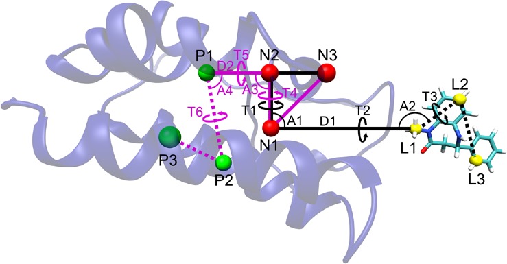
During the attachment phase, conformational, rotational, and translational restraints are applied to the protein and the ligand, starting from a system that has been equilibrated without any restraints or biases. The restraints comprise harmonic potentials applied to chosen distances, bond angles, and torsion angles, as shown in Figure 1a. As in prior work,^24,25 three atoms in both the protein and ligand are used as anchor points of the two molecules, to restrain them relative to three noninteracting, dummy anchor particles placed in strategic positions, whose Cartesian coordinates are held fixed in the lab frame. All free energy contributions from this stage are obtained by using a succession of intermediate values of the spring constants, between the unrestrained and fully restrained states, with the Multistate Bennett Acceptance Ratio (MBAR)³⁶ method to combine the multiple windows. See the Supporting Information (SI) for details.

Figure 1.

(A): Restraint scheme for the binding free energy calculations, illustrated with the ligand pulled 10 Å away from the binding site. The three noninteracting, dummy atoms, N1–N3 (red spheres), are restrained in the lab frame. Black lines define the restraints acting between the ligand’s anchor atoms (L1–L3, yellow spheres) and the dummy atoms (N1–N3). Purple lines define the restraints acting between the protein’s anchor atoms (P1–P3, green spheres) and the dummy atoms (N1–N3). D1 and D2 indicate distance restraints, and the letters A and T denote angle and dihedral (torsional) restraints, respectively. For simplicity, the three additional distance restraints between the P1–P2–P3 protein anchor atoms, and three more between the ligand L1–L2–L3 anchor atoms, are not shown. (B): The initial (left, apo closed) and final (right, apo open) states, from the pulling stage of the APR conformational calculations for the apo protein (ΔG_conf,pull). Green bars indicate the pulling reaction coordinate, which is the ψ of Asp 88, and red bars indicate the 20 torsion angles restrained in the conformational attachment phase and released after the pulling (see main text and Figure 2). The distance restraints between the protein anchor atoms P1–P3 are shown here as dotted lines.

As shown in the top panel of Figure 2, the first step in the attachment phase is attachment of the protein conformational restraints when the latter is free in solution with a bound ligand; this step corresponds to the ΔG_attach,p term. These conformational restraints are harmonic potentials applied to the three distances between the protein anchor atoms (P1–P2, P2–P3, and P1–P3) and to the Asp88N-Asp88CA-Asp88C-Ala89N (or Asp88 ψ) dihedral. The reason for this last restraint will be clarified in subsequent sections. We do not compute the free energy of attaching the translational and rotational restraints to the protein, because the work of releasing them would exactly equal the work of applying them, if fully converged. This is because the harmonic potentials applied to these coordinates (distance D2, angles A3 and A4, and torsion angles T4, T5, and T6) only keep the complex positioned and oriented in the lab frame, without influencing the conformation (i.e., the internal coordinates) of the protein–ligand system or the protein. (See Figures S1 and S2 in the Supporting Information (SI).)

Figure 2.

Steps in the free energy calculations performed in the present study. Top panel: attachment and pulling stages of the ligand binding free energy calculations, with the protein Asp88N-Asp88CA-Asp88C-Ala89N dihedral restraint shown as green bars. Middle panel: release of the conformational restraints of the apo protein, including the conformational change APR calculation, with the 20 attached dihedrals shown as the red bars. The inset shows the release of all restraints applied to the ligand. Bottom panel: release of the apo protein restraints to the metastable closed state, with the wall restraint (see text) represented by the green dotted lines.

After all protein restraints are in place, the next step is to apply all ligand restraints. This second step in the top panel of Figure 2 corresponds to ΔG_attach,l in eq 1. Harmonic potentials applied to distance D1, angles A1 and A2, and torsions T1, T2, and T3 (Figure 1a) maintain the ligand’s overall position and orientation relative to the protein (and the lab frame) during the pulling process. In order to avoid distortion of the ligand during the pulling step, conformational restraints are also applied to the distances between its anchor atoms (L1–L2, L2–L3, and L1–L3), as well as an extra dihedral for ligands 3, 4, 5, 6, 7, and 8, as shown in Figure 3. This extra restraint is used to increase the rigidity of the ligand, by not allowing the free rotation of large groups of atoms.

Figure 3.

Chemical structures of the ligands studied here (1–8). The three anchor atoms L1, L2, and L3 from each ligand are shown by the letters a, b, and c, respectively. The dihedral restraints used for ligands 3–8 are represented by the purple dotted lines. For ligand 1 we show the anchors used in the 4LYS calculations, and for ligand 8 we show the anchors and dihedral used in the 4J3I calculations.

2.1.2. Pulling Phase

With all restraints attached, the system is now ready for the pulling simulations, which bring the fully restrained ligand from the BRD4 binding site to a point in the bulk solvent far from the protein (third step in the top panel of Figure 2). The pulling free energy, ΔG_pull, is calculated by separating the distance along the pulling path between the binding site and bulk into windows and combining simulation results across the windows with MBAR. The reaction coordinate in this case is D1, the distance between one of the noninteracting anchor atoms (N1) and the L1 anchor atom in the ligand (Figure 1a). We arrange the N1, N2, and N3 atoms so that they are always in the YZ plane, and the pulling vector is parallel to the Z axis. The distance D1 is increased from 5.0 to 21 Å in 0.4 Å increments, for a total of 41 windows. We find that this window separation, combined with a pulling spring constant of k_d = 5 kcal/mol·Å², provides good overlap of sampling between the windows, including in regions in which there is a strong pulling force. At 21 Å, the protein and ligand interact negligibly, as verified by arrival at a plateau in the PMF. See Results for further details.

2.1.3. Release Phase

Once the ligand is in bulk and no longer interacting with the protein, the restraints on both molecules are released, yielding the final state in which they are separate and unrestrained. The release of the ligand (inset of the middle panel in Figure 2) can be separated into two contributions, as follows:

2

The first term on the right-hand side of the equation is the free energy change for release of the ligand conformational restraints, which is calculated using MBAR with the ligand in a separate box without any pose restraints applied to it. The second term, ΔG_{release,l–std}, is computed semianalytically:²⁴

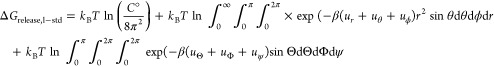3

Here C° is the standard concentration of 1 M = 1/1661 ų, and r, θ, and ϕ are distance D1, angle A1, and torsion T1 dihedral, respectively (Figure 1a). Together, these three variables define a volume element in spherical coordinates. In the last term on the right, which integrates over ligand orientation, Θ is the angle A2, Φ is the dihedral T2, and ψ is the dihedral T3. These are defined as the three Euler angles, which define the orientation of the ligand in space. The corresponding u variables are the harmonic energy functions in each restraint; e.g., for the u_r term:

4

Here k_d is the force constant applied to r, and r₀ is the reference value of the final pulling distance (21 Å). Analogous expressions apply to the restraint potentials for the angles and dihedrals. We evaluate the integrals in eq 3 numerically, without making use of molecular dynamics simulations. Because the restraints are stiff, the integrals can also be evaluated analytically, with little loss of precision, by choosing the mean values for ⟨r²⟩, ⟨sin θ⟩, and ⟨sin Θ⟩ inside the Jacobian, removing it from the integral, and integrating only the Gaussian functions.

As in the attachment phase, the free energy for release of the protein, ΔG_release,p, only includes the conformational free energy difference between the restrained and unrestrained states of the BRD4 bromodomain. The ligand at this stage is assumed to be far enough away from the protein that it can be omitted from the protein release calculation. However, a complicating factor arises, as our simulations point to a slow conformational change of the protein, subsequent to removal of the ligand, from what we call the ”closed” to the ”open” state (Figure 1b). The former is stable in the presence of the ligand but only metastable in the apo state in the absence of protein conformational restraints. In principle, the free energy contribution of the relaxation from closed to open could be included in ΔG_pull, since the binding site opens once the ligand is out. However, waiting for this slow process to occur during the pulling step for every ligand would make the binding calculations much more time-consuming. To avoid this cost, we modified the calculation so that the free energy change associated with this conformational change needs to be computed only once.

To do this, we included a harmonic restraint on the Asp88 backbone ψ (or Asp88N-Asp88CA-Asp88C-Ala89N) dihedral angle as one of the protein restraints (see above, and Figure 2, green bars on top panel). This is sufficient to keep the protein closed in all attaching and pulling windows, and its use means that the protein is still restrained in the closed state at the end of each ligand pull (Figure 2, last configuration in top panel). Because the protein is in the same closed, restrained, apo state at the end of each ligand pull, the reversible work of releasing all protein restraints, ΔG_release,p, needs to be computed only once, for this final protein state. We compute ΔG_release,p via what may be viewed as another set of attach, pull, and release steps (Figure 2, middle panel):

5

The first term on the right-hand side is the change in free energy on attaching additional conformational restraints that stabilize the structure during the conformational pulling phase, and the second and third terms are the free energies for the conformational pulling and releasing stages, respectively.

The attachment free energy ΔG_conf,attach is associated with the imposition of 20 new restraints, on all ϕ and ψ backbone torsions in the protein’s ZA-loop (Pro86 to Tyr98), except for Asp 88 ψ (Figures 1 and 2), which is already restrained, as well as Asp 88 ϕ and Asp 96 ϕ and ψ. Together, these two residues represent the hinges of the apo BRD4 closed to open transition (Figure 1b). Note that the harmonic restraints on the three P1 to P3 distances are also present at this stage. The Asp88 ψ dihedral is used as the reaction coordinate for the pulling stage (ΔG_conf,pull), during which the conformation is shifted from closed to open. This dihedral restraint has a reference value of 80 degrees when the BRD4 bromodomain is in the closed state and −40 degrees when the protein is in the open state. We separate this range into 10 degrees intervals, for a total of 13 pulling windows. After the pulling process, the domain is in the stable, open apo state, and we can release all the remaining restraints on the protein (ΔG_conf,release), i.e., those on the 20 recently attached dihedrals, Asp88 ψ, and the three anchor atom distances. All free energies from the calculation of eq 5 are obtained using MBAR, either varying the spring constants or the reference value of the harmonic restraint applied to the reaction coordinate. (See the SI for details.)

2.1.4. Free Energy of the Protein Conformational Change

Interestingly, as noted above, the stable, open state of the apo BRD4 bromodomain from our simulations is not consistent with apo crystal structures of this protein in the apo state,^37,38 as the latter has the same conformation as when a ligand is bound (closed state), shown in Figure 1b. This difference might stem from inaccuracies in the simulations or, alternatively, from crystal packing artifacts. We further characterized this conformational change by computing its associated free energy change. This was done by computing a second free energy of protein release, ΔG_{release,p,closed}, this time to the closed, rather than the open state (Figure 2, lower panel). Because ΔG_release,p and ΔG_{release,p,closed} start from the same initial state (the restrained protein) and end at the open and closed states, respectively, their difference is the desired free energy of the conformational change:

6

We computed ΔG_{release,p,closed} as the reversible work of releasing all restraints on the protein, except for a new wall-like restraint on ψ of Asp88, positioned to prevent this angle from going lower than 55 degrees. This restraint still allows local fluctuations of this dihedral but does not permit the transition to the apo open state. Note that substituting ΔG_{release,p,closed} for ΔG_release,p in eq 1 yields the free energy of ligand binding under an assumption that the protein does not transition to its open conformation after the ligand is out. This quantity is termed ΔG_bind,closed^°, and we have ΔG_bind = ΔG_bind,closed^° – ΔG_conf,p.

2.2. Chemical Structures and Simulation Methods

We focus on seven ligands that are so chemically dissimilar from each other that it would likely be impractical to compute their relative binding free energies by alchemical methods.¹⁶Figure 3 shows these compounds, along with each one’s three anchor atoms and the dihedrals restrained in five of the seven. All ligands were considered to be nonionized. We started the APR calculations with the crystal structures of the BRD4 bromodomain-ligand complexes, which for ligands 1–7 have PDB IDs 4LYS (XD1),³⁸4HBV (quinazolin),³⁹4PCI (B16),³³3U5L (BZT-7),⁴⁰4MR3 (RVX-OH),⁴¹5CQT (compound 28),⁴² and 4LRG (compound 3),⁴³ respectively (Figure 3).

We also tested the ability of APR calculations to correctly rank various ligand poses. For ligand RVX-208 (Figure 3, ligand 8), we used both the appropriate cocrystal structure, 4J3I,⁴⁴ and the cocrystal structure of the highly similar compound RVX-OH, 4MR3. In the latter case, we used the RVX-OH ligand as a template to position RVX-208 in the corresponding binding pose, which differs significantly from the correct pose of RVH-208 in 4J3I. We also docked ligand XD1 to the BRD4 bromodomain, using the program Dock6.7 and the 4LYI apo crystal structure, setting a minimum of 3.0 Å difference in the RMSD between the reported binding modes to ensure that distinctly different poses would be available for evaluation by APR.

For simulations of the apo BRD4 bromodomain, we used the crystal structures with PDB codes 4LYI(38) and 2OSS.³⁷ The protonation states for the protein residues were set to physiological pH of 7.4, with negative charges on all aspartate and glutamate side chains, as well as on the protein C-terminus, and positive charges on all lysine and arginine side chains, as well as on the N-terminus. The parameters for all the ligands were set using either the Amber General Force Field (GAFF), or the recent update GAFF2, with the AM1-BCC charge model⁴⁵ for the atomic point charges. For the protein, we used the ff14SB parameters⁴⁶ with three different models for water: TIP3P,²⁸ TIP4PEw,²⁹ and SPC/E,³⁰ with the Joung and Cheatham ion parameters for each of the three water models.⁴⁷

Simulations of the protein–ligand complexes and the apo protein included 11,000 water molecules, 32 Na⁺ ions, and 35 Cl^– ions, in order to produce a NaCl concentration of 0.15 M. The box size of the protein systems after equilibration was approximately 60 Å × 60 Å × 100 Å, and we used periodic boundary conditions on the three axes. Simulations of the solvated ligand alone were run in a periodic box of about 40 Å × 40 Å × 40 Å, with the same NaCl concentration of 0.15 M. All simulations were performed using the pmemd.cuda program from either AMBER14 or AMBER16, the latter being employed for the runs with GAFF2 parameters. Production runs were performed in the NPT ensemble, with temperature control at T = 298.15 K using a Langevin thermostat⁴⁸ with collision frequency of 1.0 ps^–1, as well as pressure control at 1 bar provided by the Monte Carlo barostat.⁴⁹ Nonbonded interactions had a cutoff of 9.0 Å, and the long-range electrostatics were calculated using the PME method.⁵⁰ Bonds involving hydrogen were constrained by using the SHAKE algorithm,⁵¹ and we used a 4 fs time step with hydrogen mass repartition (HMR).⁵² The HMR method works by repartitioning the masses of heavy atoms into the bonded hydrogen atoms, allowing the time step of the simulation to be increased by up to a factor of 2. For that purpose, AMBER’s parmed.py program was used to edit the system’s parameter/topology file, increasing the hydrogen masses to 3.024 Da and reducing the mass of neighboring heavy atoms by the same amount, but without altering the water molecules. The three dummy particles, N1, N2, and N3, were assigned zero charge, and zero Lennard-Jones radius and well-depth, and a mass of 220 Da, and their Cartesian coordinates were restrained by an harmonic force constant of k = 50 kcal/(mol·Å²).

The preparation of the system before the equilibration and production runs started with the creation of the simulation box and initial energy minimization, with positional restraints kept on both the protein and the ligand. We then slowly heated the system over 1 ns, at constant volume, 10–298.15 K, and equilibrated the system in the NPT ensemble for 1.0 ns. Subsequent simulations started from this point. Each window in the attachment and release stages of the binding free energy calculations was simulated for 40 ns, with 15 ns of equilibration and 25 ns of data collection. Each window in the pulling stages, as well as the attaching and releasing stages of the conformational change calculations, was simulated for a total time of 140 ns, comprising 40 ns of equilibration and 100 ns of data collection. Each simulation used a single GeForce GTX Titan X Graphics Processing Unit, running at 200 ns/day. The net simulation time to compute the binding free energy for a single ligand and one set of force field parameters, not counting the protein conformational change, which was done once for all ligands, is 7.54 μs. This would take about 38 days of serial processing on a single GPU, but much less wall clock time was actually needed because different components of the APR calculations were trivially run in parallel. The total simulation time of the present work is approximately 300 μs or 0.3 ms.

3. Results

This section presents binding free energies for the first BRD4 bromodomain with seven chemically diverse ligands, computed with the TIP3P, TIP4PEw, and SPC/E water models, each in conjunction with both GAFF and GAFF2 parameters for the ligands, for a total of six force field combinations. We assess numerical convergence, compare the results with experiment, and examine the free energy changes associated with each step in the APR process. We first focus on results where the protein is released to its more stable, open conformation. The protein conformational change then is analyzed in the last subsection. The detailed results of each step in the APR calculations for all ligands and parameters are provided in the SI.

3.1. Binding Free Energy Calculations

The calculated binding free energies correlate with experiment (Figure 4 (red circles), Table 1 and Table S8), with Pearson correlation coefficients ranging from 0.55 (TIP3P-GAFF2) to 0.83 (SPC/E-GAFF). Additionally, the slopes of linear regression fits are near unity (0.98–1.18) for four force fields, including SPC/E-GAFF. The TIP3P and TIP4PEw consistently overestimate (closer to zero) the binding free energies, with mean signed errors (MSE) of 2.54–2.88 kcal/mol, whereas the SPC/E water model yields less biased results, with MSE values of 0.91 and 1.18 kcal/mol for GAFF and GAFF2, respectively. Overall, the combination of SPC/E water and the GAFF force field yields the best agreement with experiment (RMSE 1.42 kcal/mol), and the results for SPC/E with GAFF2 are only slightly worse (RMSE 1.66 kcal/mol). All of the TIP3P and TIP4PEw results are significantly less accurate (RMSE 2.77–3.21 kcal/mol). The differences between calculations with GAFF versus GAFF2 are less marked, and less consistent, than those between calculations with different water models. Note that the same AM1/BCC charges are used here with both GAFF and GAFF2.

Figure 4.

Scatter plots of computed versus experimental free energies. Ligands 7–1 are displayed in sequence from left to right in each graph, as this is the order of decreasing affinity, with red circles representing calculations that account for the free energy of the protein’s closed-to-open conformational change, and black squares representing calculations where the protein remained in its closed state. (A): The TIP3P water model with GAFF parameters. For three of the ligands, binding free energies previously computed by an alchemical method¹¹ are shown as green diamonds. (B): Same as (A), but using the GAFF2 parameters for the ligands. (C,D): Same as A,B, respectively, except using the TIP4PEw water model. (E,F): Same as A,B, respectively, except using the SPC/E water model.

Table 1. Experimental and Calculated Standard Binding Free Energies, ΔG_bind^°, for the Various Ligands and Parameters, Using the Open State as the Final Apo State of the Protein^a.

Affinities
ligand	exp.	TIP3P-GAFF	TIP3P-GAFF2	TIP4P-GAFF	TIP4P-GAFF2	SPC/E-GAFF	SPC/E-GAFF2
1	–5.95b38	–4.59	–4.67	–4.23	–4.15	–5.93	–5.20
2	–6.36c11,39	–3.05	–2.65	–1.93	–1.72	–3.82	–3.64
3	–7.01c33	–4.81	–4.44	–2.64	–2.78	–5.17	–5.70
4	–8.16b40	–7.53	–8.07	–8.05	–7.82	–9.22	–9.26
5	–8.99b41	–6.35	–5.17	–6.04	–6.38	–8.12	–8.33
6	–9.45c42	–5.62	–4.67	–5.55	–5.89	–8.31	–7.84
7	–10.41c43	–6.57	–6.89	–7.72	–7.96	–9.36	–8.08

Statistics
	exp.	TIP3P-GAFF	TIP3P-GAFF2	TIP4P-GAFF	TIP4P-GAFF2	SPC/E-GAFF	SPC/E-GAFF2
MSE	0.00	2.54	2.82	2.88	2.80	0.91	1.18
RMSE	0.14	2.77	3.18	3.21	3.10	1.42	1.66
y-int	–0.02	–0.49	–0.67	3.42	4.17	1.70	0.91
slope	1.00	0.63	0.58	1.07	1.18	1.10	0.98
r	1.00	0.69	0.55	0.73	0.78	0.83	0.77
τ	0.89	0.43	0.33	0.40	0.44	0.49	0.38

^aSummary statistics at the bottom of the table are the root mean squared error (RMSE), mean signed error (MSE), the y-intercept (y-int) and slope of a linear regression fit of calculation and experiment, the Pearson’s correlation coefficient (r), and the Kendall τ between the experimental and the calculated values. The statistics are estimated using 100,000 bootstrap samples with replacement of the 7 ligands, where both the experimental and computed results are drawn from Gaussian distributions centered on the reported means and having standard deviations of the standard errors of the mean for both calculation and experiment. (The standard errors are provided in Table S8.) The statistics listed in the exp. column are based on bootstrapping of experimental results against themselves and thus give a sense for the best possible results one might expect from any computational method.

^bObtained by isothermal titration calorimetry.

^cObtained using Alphascreen.

The numerical uncertainties of the computed binding free energies, reported as standard errors of the mean, are modest, at 0.16–0.35 kcal/mol (Table S8). These values are similar in magnitude to typically reported experimental uncertainties. The low numerical uncertainties reflect good convergence of the work calculations carried out to implement the APR method. Further information regarding convergence is provided in Figure 5, which shows the convergence of the potentials of mean force, and histograms with good overlap between umbrella sampling windows, for the example of ligands 4 and 7 with the SPC/E-GAFF calculations.

Figure 5.

Sample convergence and overlap results, for simulations with the SPC/E water model and the GAFF parameters for the ligand. (A,B): Convergence of the ΔG_pull term for the binding free energy calculations of ligands 4 and 7, respectively. Each line corresponds to a different amount of simulation time per window (see inset legends), with the solid black lines denoting the final results. (C,D): Histograms of the first 30 pulling windows (ΔG_pull) for the binding free energy calculations of ligands 4 and 7, respectively.

It is of interest to examine the five individual work terms that go into making up each computed binding free energy (eq 1). These are shown in Figure 6, along with net computed and experimental binding free energies. In all cases, the pulling work, ΔG_pull, is the largest term, strongly opposing extraction of the ligands from the binding site across all force field combinations. The attachment terms are consistently unfavorable, as expected for the attachment of restraints, and the release terms are consistently favorable. Interestingly, for both the ligand and protein, the favorability of release consistently outweighs the cost of attachment. (The work of protein release is discussed in more detail below.) The pulling phase additionally provides most of the variation among ligands. Indeed, the protein attachment work is nearly independent of what ligand is bound, and the protein release work is, in fact, entirely independent of ligand; see Figure 2. The work of attachment and release varies more across ligands but still not as much as the pulling work. Note that much of the ligand release work is computed analytically and does not depend on the force field or ligand parameters.

Figure 6.

Free energies associated with the steps of the APR calculations, as labeled, along with the negative of the corresponding experimental results (−Expt) and the final computed (−Calc Bind) results accounting for the closed-to-open conformational transition. In each panel, results are shown for each of the seven ligands (colored uniquely), displayed from left to right; uncertainties are shown as error bars. (A): The TIP3P water model with GAFF parameters. (B): The TIP3P water model with GAFF2 parameters. (C,D): Same as A,B, respectively, but for the TIP4PEw water model. (E,F): Same as A,B, respectively, but for the SPC/E water model.

3.2. Conformational Change of the Apo Bromodomain

In the present simulations, the BRD4 bromodomain goes through a spontaneous conformational transition in the absence of bound ligand, from closed to open, as shown in Figure 1. This holds for all three water models examined. (The choice of GAFF versus GAFF2 is irrelevant, because the ligand is absent from the apoprotein.) We first noticed opening of the apoprotein ZA-loop during exploratory pulling calculations lacking the Asp88N-Asp88CA-Asp88C-Ala89N dihedral restraint. Opening occurred typically between 20 and 60 ns, for windows with the ligand far from the binding site. We then ran unrestrained simulations starting from the apo BRD4 bromodomain crystal structures 4LYI and 2OSS, for all three water models, and observed the same conformational transition (Figure S3). In all cases, this change was found to be irreversible, even after hundreds of nanoseconds of simulations. Interestingly, the protein is found to be in the closed state in both apo crystal structures (PDB 4LYI and 2OSS).

The opening event is associated with distinct transitions in the main chain torsion angles of Asp 88 and Asp 96, as seen near the 50 ns mark of an exemplary 300 ns simulation of the apoprotein (Figure 7a). In contrast, the distributions of the other 20 main chain torsions in the ZA-loop change minimally during the transition (Figure 7b,c). The main chain torsions of Asp 88 and Asp 96 thus act as the hinges of the closed to open transition. We find, accordingly, that applying a harmonic restraint with a force constant of k_t = 20 kcal/(mol·rad²) to Asp 88 ψ, with a reference value corresponding to the closed state (80 degrees), suffices to prevent the opening transition. As discussed in Methods, this restraint was used to prevent opening during the attachment and pulling phases.

Figure 7.

Simulated time series of the torsion angles involved in the closed to open transition. All results are based on the initial 4LYI apo crystal structure and the TIP3P water model. (A): Time-series of Asp 88 ϕ and ψ backbone torsions (black and red, respectively), and Asp96 ϕ and ψ (green and blue, respectively), during a 300 ns unrestrained simulation of apo BRD4 bromodomain. The closed to open conformational transition occurs at about 50 ns. (B,C): Time series of the 20 additional dihedrals restrained in the ΔG_conf,attach calculation, during the same unrestrained 300 ns simulation as in panel (A); ten of the 20 are displayed in each graph. (D): Time series of the same dihedrals in (A) but now from a 30 ns steered MD simulation in which ψ of Asp88 is driven from 80 to −40 degrees.

The Asp 88 ψ dihedral also serves as a reaction coordinate to obtain the free energy change associated with the conformational change. Thus, a steered MD simulation in which the reference value of this restraint is changed from 80 (closed) to −40 degrees (open) leads to corresponding transitions of the other hinge torsions (Figure 7d). This simulation was also used to define initial windows for the calculation of ΔG_conf,pull. Potentials of mean force along this coordinate have initial and final energy energy wells separated by a barrier of ∼2 kcal/mol, for all three water models. For TIP3P (Figure 8a) and TIP4PEw (Figure 8b), the wells corresponding to the open state are lower than for the closed state, particularly for TIP4PEw, but they are similar in energy for SPC/E (Figure 8c). It is also evident from the families of curves shown that these PMFs converge well, also showing good overlap between the conformational pulling windows (Figure 8d). When combined with the free energies of attachment and release associated with this conformational transition (see Methods), and with the free energy of protein release to the closed state (below), the open state is found to be more favorable than the closed state by −2.54, −3.72, and −1.67 kcal/mol, for TIP3P, TIP4Ew, and SPC/E, respectively. The stepwise breakdown of these values is provided in the SI.

Figure 8.

Convergence and histogram overlap for the ΔG_conf,pull stage of the apo BRD4 conformational transition calculations. Each line corresponds to a different simulation time per window (see inset legend), with the solid black line denoting the final results. (A,B,C): results for the TIP3P, TIP4PEw, and SPC/E water models, respectively. (D): Overlap of the reaction coordinate histograms from the 13 windows used in the ΔG_conf,pull calculation with TIP3P.

We used the fact that Asp 88 ψ is a control variable⁵³ for the conformational change to compute a new set of protein release free energies where the protein remains in its closed form. This was done by carrying out the release calculations in the presence of a wall restraint keeping Asp 88 ψ within its ”closed” energy well without significantly perturbing fluctuations within the closed state (Figure S4). The resulting free energy of protein release is termed ΔG_{release,p,closed}, the corresponding binding free energy is termed ΔG_bind,closed^°, and the free energy of the opening transition, ΔG_conf,p, is obtained from eq 6. Note that the free energy of the conformational change is independent of the ligand, so that ΔG_bind,closed for every ligand is the same as the corresponding value ΔG_bind^° except for a shift by ΔG_conf,p:

7

The values of ΔG_bind,closed^° are compared with experiment in Table 2, Table S9, and Figure 4 (black squares). Referencing the closed conformation only produces a uniform shift in the computed results, so the correlations between experiment and calculation are essentially unchanged. However, because the opening transition of the apo protein is thermodynamically favored, and thus favors dissociation, trapping the protein in the closed end state causes the binding free energies to be more favorable (more negative). The net effect is to reduce the bias in the computational results and generate improved agreement with experiment, in particular for the TIP3P and TIP4PEw calculations.

Table 2. Same as Table 1 but Using the Metastable Closed State as the Final Apo State of the Protein, so That the Computed Free Energies Here Are ΔG_bind,closed^°a.

Affinities
ligand	exp.	TIP3P-GAFF	TIP3P-GAFF2	TIP4P-GAFF	TIP4P-GAFF2	SPC/E-GAFF	SPC/E-GAFF2
1	–5.95b38	–7.13	–7.21	–7.95	–7.87	–7.60	–6.87
2	–6.36c11,39	–5.59	–5.19	–5.65	–5.44	–5.49	–5.31
3	–7.01c33	–7.35	–6.98	–6.36	–6.50	–6.84	–7.37
4	–8.16b40	–10.07	–10.61	–11.77	–11.54	–10.89	–10.93
5	–8.99b41	–8.89	–7.71	–9.76	–10.10	–9.79	–10.00
6	–9.45c42	–8.16	–7.21	–9.27	–9.61	–9.98	–9.51
7	–10.41c43	–9.11	–9.43	–11.44	–11.68	–11.03	–9.75

Statistics
	exp.	TIP3P-GAFF	TIP3P-GAFF2	TIP4P-GAFF	TIP4P-GAFF2	SPC/E-GAFF	SPC/E-GAFF2
MSE	0.00	0.00	0.28	–0.84	–0.92	–0.76	–0.49
RMSE	0.14	1.14	1.53	1.61	1.61	1.29	1.23
y-int	–0.02	–3.03	–3.23	–0.30	0.45	0.03	–0.77
slope	1.00	0.63	0.57	1.07	1.18	1.10	0.98
r	1.00	0.70	0.55	0.74	0.79	0.83	0.77
τ	0.89	0.44	0.33	0.40	0.44	0.50	0.38

^aThe uncertainties are shown in Table S9. Note that the values of r, τ, and slope can be slightly different from those in Table 1, due to the stochastic nature of the bootstrapping procedure.

^bObtained by isothermal titration calorimetry.

^cObtained using Alphascreen.

The values of ΔG_bind,closed^° for TIP3P-GAFF agree closely with previous calculations¹¹ for ligands 2, 4, and 5 (Figure 4a, green diamonds), which used the same water and ligand parameters and a similar protein force field, Amber99SB-ILDN,⁵⁴ but an alchemical decoupling free energy method¹⁹ instead of the present APR method. Our values of ΔG_bind are offset from ΔG_bind,closed^°, and hence from the prior results, by the free energy of the closed-to-open conformational change. Accordingly, the relative values of ΔG_bind still agree well with the prior results. We conjecture that the differences between the present and prior results for these compounds derive from a difference in how the closed-to-open conformational change of the protein was handled. Overall, it is encouraging that two entirely independent studies obtained very similar results for matched cases.

3.3. Application to Ligand Docking

Because molecular dynamics simulations of protein–ligand complexes do not efficiently sample varied ligand poses, free energy simulations report only on the binding free energy associated with the ligand pose used to initiate the calculations. However, in many practical settings, one does not know the true pose in advance. One potential solution to this problem would be to initiate free energy calculations from the top-ranked pose provided by a fast docking algorithm, but this risks making the more detailed free energy calculations reliant upon relative crude docking calculations. It is therefore of interest to examine whether the APR method can be used to select the most stable pose from multiple plausible poses generated by a docking code or other low-resolution methods.

As an initial test, we used the APR method to compute the binding free energy of ligand 1 (XD1) in the three top scoring binding poses provided by Dock6.7 (see Methods), using the SPC/E-GAFF set of parameters, which had provided the best agreement with experimental binding affinities (see above). The APR calculations indicate that the most stable (highest affinity) pose is the one ranked second according to Dock6.7, with a binding free energy around 1.5 kcal/mol lower than the other two (Table 3). This pose is also the one that produces the best agreement with the crystal structure of the complex, with an RMSD of 1.23 Å (Figure S5). Interestingly, the calculated affinity for this docked pose is also higher than the one calculated from the reference crystal structure (Table 3). It is not yet clear why a pose docked into the apoprotein structure led to a greater computed affinity than the true cocrystal structure. The RMSDs of poses ranked 1 and 3 compared to the 4LYS structure are 6.44 and 5.41 Å, respectively (Figure S5 and Table 3). They also have a slightly lower affinity then the one obtained from this crystal structure, but this value is inside the associated errors from our calculations. In all docked poses, unrestrained simulations of the complex showed no transition of BRD4 to the open state, which was also the case for all the other ligands.

Table 3. Calculated Affinities, and Comparison with Experimental Values, for the XD1 and the RVX-208 Ligands Using Different Binding Poses.

pose	pose RMSD (Å)	ΔGbind (calc)	ΔGbind (expt)
Ligand XD1
dock rank 1	6.44	–5.41 (0.26)	–5.95 (ND)38
dock rank 2	1.23	–6.74 (0.30)
dock rank 3	5.41	–5.18 (0.28)
cocrystal	0.00	–5.93 (0.27)
Ligand RVX-208
cocrystal A	0.00	–6.34 (0.32)	–6.93 (ND)44
cocrystal B	1.42	–5.52 (0.30)
modeled on RVX-OH	7.45	–5.06 (0.32)

We also tested whether APR calculations with the same force field parameters could distinguish correct from incorrect binding poses of ligand 8, RVX-208. This molecule is very similar to RVX-OH (Figure 3), but it binds to the BRD4 bromodomain in a completely different mode (Figure S5), and it is interesting to ascertain whether the APR calculations can reproduce this behavior. In Table 3 we show the value for the binding free energies of the RVX-208 ligand in three different poses. The first two, called 4J3I-A and 4J3I-B, are from the crystal structure of RVX-208 in complex with the first BRD4 bromodomain and are very similar to each other (Figure S5). The third has the same binding mode as RVX-OH and is based on the 4MR3 crystal structure solved with that ligand. We can see that the two poses from the crystal structure of RVX-208 provide values for the binding free energies that are lower (higher affinity) than the one obtained from the RVX-OH structure. This difference is small in the case of the 4J3I-B but has a value of around 1.3 kcal/mol in the case of 4J3I-A. Thus, the free energy calculations successfully distinguish the correct binding mode.

4. Discussion

4.1. Method and Accuracy

We report here the first application of the APR free energy formalism to protein–ligand binding, in calculations of the absolute (standard) binding free energies of seven chemically diverse ligands to the first BRD4 bromodomain. Binding free energies apparently converged to within a few tenths of a kcal/mol standard error of the mean are readily obtained. We took advantage of the efficiency of the present approach to explore how the accuracy, relative to experiment, depends on the potential function, across all six combinations of three water models (TIP3P, TIP4PEw, SPC/E) and two ligand parameter sets (GAFF and GAFF2). The SPC/E water model with GAFF parameters yielded the most accurate results (RMSE of 1.42 kcal/mol), while both TIP water models led to systematic underestimates of the binding affinities. Nonetheless, even the worst correlation coefficient across all models, 0.55, is still reasonably good, and we would not assume that SPC/E model will outperform the TIP models for other protein–ligand systems.

Perhaps unexpectedly, the overall accuracy of these and other^{10,11,15,55,56}absolute binding free energy calculations is similar to that reported for relative binding free energy calculations requiring alchemical transformations between ligands.^16,57,58 If this holds true in future work, then absolute free energy methods, such as APR, may ultimately be preferred, because, unlike relative free energy methods, they do not require that the ligands be chemically similar to each other. In addition, APR and some other absolute methods (see below) can be run with simulation codes that are not equipped to carry out alchemical transformations.

It is also of interest to put the present results into the context of recent blinded prediction challenges. Part of a recent D3R challenge⁵⁹ focused on ligand binding free energy predictions of three subsets of 5, 4, and 10 druglike molecules to the protein HSP90. The computational methods used spanned alchemical free energy methods, fast scoring functions, and electronic structure calculations. The RMSE values for the SPC/E-GAFF parameters are similar to those of the top ranked submissions for two of the three free energy challenge subsets, whereas the other set had submissions with RMSE values under 1 kcal/mol. Although the present Kendall τ value of 0.49 is higher than those of all D3R submissions for the binding free energy stage, this difference could result, at least in part, from the greater spread of free energies in the present study, as this makes the rankings less sensitive to small errors in the computed free energies. In addition, somewhat to our surprise, the accuracy found here for the BRD4 bromodomain is at least as good as that obtained when the APR method was applied to a series of far simpler host–guest systems in the SAMPL5 challenge.²⁵ However, it should be noted that the present study is retrospective, in the sense that the experimental results were known to us at the time we made the calculations. It will be informative to challenge it in the more stringent setting of blinded predictions.

4.2. Accounting for Protein Conformational Change

In the course of this study, we identified a spontaneous closed-to-open conformational change, occurring typically after 20–60 ns of simulation of the apo protein. This delayed opening event must be accounted for, as it affects the binding free energies, but waiting for it to occur as each ligand is pulled from the binding site would have significantly increased the computational cost. We addressed it instead through an extension of the APR approach, involving a one-time evaluation of the PMF for the opening process. This yields a single free energy correction term for the opening transition, which is applicable to all seven ligands. We also computed the seven binding free energies under an assumption that the metastable closed apo conformation does not open. These results agree particularly well with prior calculations for three of these binding reactions that were obtained by an alchemical decoupling method¹¹ using a very similar force field. It would be interesting to know whether the closed-to-open transition occurred in the prior calculations.

4.3. Perspective and Directions

The present study focuses on the calculation of standard¹⁹ or ”absolute”⁶⁰ binding free energies, rather than using alchemical methods to compute the relative binding free energies of different ligands.⁶¹ On one hand, relative binding free energy methods may require less conformational sampling, because changing one ligand into another similar one is a smaller change in the system than extracting a ligand from the binding site, which is required for absolute binding free energy calculations. On the other hand, alchemical transformations between ligands pose increasing technical challenges as the ligands become less chemically similar⁵⁸ and if they are of different net charges.^62,63 Thus, absolute binding free energy methods promise to be particularly relevant in applications like virtual screening of diverse chemical libraries, where they may provide a computationally intensive final screen of high-scoring compounds suggested by fast docking methods.

Absolute binding free energy methods, in turn, may be divided into two groups:⁵⁵ those which use an alchemical approach to effectively extract the ligand from the binding site, such as the Double Decoupling Method (DDM),^19,64 and methods in which the ligand is extracted along a physical pathway,¹² such as the present APR method. Again, each is expected to have its own advantages. One one hand, the DDM avoids the potentially challenging requirement of defining a physical path for the ligand to exit the binding site; this may be particularly problematic when the ligand is deeply buried. (However, it is worth noting that the DDM may also have problems with buried binding sites, as there is usually a requirement for water to penetrate and reoccupy the site after the ligand is gone.) On the other hand, physical pathway methods can be used in codes that are not outfitted to run alchemical calculations, and they avoid potential problems with changes in net system charge that can arise in some DDM implementations. It is worth noting that enhanced sampling methods, such as metadynamics¹⁴ and adaptive force bias,²⁰ have been used to efficiently compute absolute binding free energies using physical paths. Our implementation of the APR method does not take advantage of such enhanced sampling algorithms but instead capitalizes on the high performance of the pmemd.cuda module of AMBER. This allows for thorough sampling of the various windows at low computational cost.

All physical path methods are most readily applied when the ligand binds at the surface of the protein, so that it has an unobstructed path to the solvent. However, it should also be possible to apply physical path methods to systems where the ligand is occluded from the solvent, by attaching conformational restraints to elements of the protein and using them to pull open the binding site. After the ligand has been pulled out into bulk solvent, the binding site can be moved to its apo conformation and the restraints released. This last calculation needs to be performed only once for each protein to take care of all ligands. (It may also be omitted, if one is interested only in relative binding free energies, as it adds the same correction term to every ligand’s binding free energy.) Although these steps will add complexity, and it may be difficult to automate their setup, it should be possible to set them up just once for a given protein and then apply the same procedure repeatedly for all ligands of interest. It is also worth noting that applying the DDM method to ligands in a buried binding site may require its own specialized steps to let water enter and equilibrate in the vacated site and to account for any conformational change when the protein goes to its apo state.

Running the APR method requires the usual protein preparation steps (e.g., defining protonation states and dealing with missing atoms), definition of simulation parameters (e.g., box size, nonbonded cutoffs), selection of anchor atoms, and selection of any desired protein and ligand restraints. We have developed automated scripts to handle the entire procedure, which are currently being developed for public release. They include the setup of simulation systems, execution of the simulations, and analysis of the results for each ligand. A sample calculation for the BZT-7 ligand, including the automated scripts, has been made available for public access.⁶⁵ This level of automation greatly facilitates applications to test force fields and evaluate ligands, and we plan to broaden the protein–ligand test set and evaluate further parameter options spanning protein force fields, additional water models, and protocols for choosing atomic point charges.

Although the main goal of this work is to develop and evaluate the APR method for calculation binding free energies, we have also carried out a preliminary assessment of its potential as a physics-based docking refinement protocol, much as recently done with a different free energy method.¹⁸ Encouragingly, in both test cases, the poses with the lowest calculated binding free energy were consistent with the crystal structure of the respective protein–ligand complexes, even when the docking program used to generate the candidate poses ranked them incorrectly. We are currently working on maximizing the efficiency of this protocol so that it may be fully integrated with docking procedures. Our goal is to create an integrated workflow which may be used to screen compound libraries for high affinity ligands for the BRD4 bromodomain and other proteins. To accomplish this, we will automate the choice of anchor atoms in the ligands; and to maximize efficiency, we will implement code to monitor for convergence in each simulation window, so that sampling may be halted once sufficient sampling is achieved. These added features will greatly expand the applicability of the method.

Supporting Information Available

The Supporting Information is available free of charge on the ACS Publications website at DOI: 10.1021/acs.jctc.7b00275.

• Details on the ligand binding free energy protocol, the complete results for each ligand, and the analysis of the protein conformation in the apo and bound states (PDF)

M.K.G. thanks the NIH for partial support of this work through grant R01GM061300.

Disclosure: The contents of this publication are solely the responsibility of the authors and do not necessarily represent the official views of the NIH.

The authors declare the following competing financial interest(s): M.K.G. has an equity interest in and is a cofounder and scientific advisor of VeraChem LLC.

References

- Bird A. Perceptions of epigenetics. Nature 2007, 447, 396–398. 10.1038/nature05913. [DOI] [PubMed] [Google Scholar]
- Kouzarides T. Chromatin Modifications and Their Function. Cell 2007, 128, 693–705. 10.1016/j.cell.2007.02.005. [DOI] [PubMed] [Google Scholar]
- Strahl B. D.; Allis D. The language of covalent histone modifications. Nature 2000, 403, 41–45. 10.1038/47412. [DOI] [PubMed] [Google Scholar]
- Chung C. Small Molecule Bromodomain Inhibitors: Extending the Druggable Genome. Prog. Med. Chem. 2012, 51, 1–55. 10.1016/B978-0-12-396493-9.00001-7. [DOI] [PubMed] [Google Scholar]
- Jang M. K.; Mochizuki K.; Zhou M.; Jeong H.-S.; Brady J. N.; Ozato K. The Bromodomain Protein Brd4 Is a Positive Regulatory Component of P-TEFb and Stimulates RNA Polymerase II-Dependent Transcription. Mol. Cell 2005, 19, 523–534. 10.1016/j.molcel.2005.06.027. [DOI] [PubMed] [Google Scholar]
- Filippakopoulos P.; Qi J.; Picaud S.; Shen Y.; Smith W. B.; Fedorov O.; Morse E. M.; Keates T.; Hickman T. T.; Felletar I.; Philpott M.; Munro S.; McKeown M. R.; Wang Y.; Christie A. L.; West N.; Cameron M. J.; Schwartz B.; Heightman T. D.; Thangue N. L.; French C. A.; Wiest O.; Kung A. L.; Knapp S.; Bradner J. E. Selective inhibition of BET bromodomains. Nature 2010, 468, 1067–1073. 10.1038/nature09504. [DOI] [PMC free article] [PubMed] [Google Scholar]
- Nicodeme E.; Jeffrey K. L.; Schaefer U.; Beinke S.; Dewell S.; Chung C.; Chandwani R.; Marazzi I.; Wilson P.; Coste H.; White J.; Kirilovsky J.; Rice C. M.; Lora J. M.; Prinjha R. K.; Lee K.; Tarakhovsky A. Suppression of inflammation by a synthetic histone mimic. Nature 2010, 468, 1119–1123. 10.1038/nature09589. [DOI] [PMC free article] [PubMed] [Google Scholar]
- Mirguet O.; Gosmini R.; Toum J.; Clement C. A.; Barnathan M.; Brusq J.-M.; Mordaunt J. E.; Grimes R. M.; Crowe M.; Pineau O.; Ajakane M.; Daugan A.; Jeffrey P.; Cutler L.; Haynes A. C.; Smithers N. N.; Chung C.-w.; Bamborough P.; Uings I. J.; Lewis A.; Witherington J.; Parr N.; Prinjha R. K.; Nicodeme E. Discovery of Epigenetic Regulator I-BET762: Lead Optimization to Afford a Clinical Candidate Inhibitor of the BET Bromodomains. J. Med. Chem. 2013, 56, 7501–7515. 10.1021/jm401088k. [DOI] [PubMed] [Google Scholar]
- Chipot C. Frontiers in free-energy calculations of biological systems. Wiley Interdiscip. Rev.:Comput. Mol. Sci. 2014, 4, 71–89. 10.1002/wcms.1157. [DOI] [Google Scholar]
- Heinzelmann G.; Chen P.-C.; Kuyucak S. Computation of Standard Binding Free Energies of Polar and Charged Ligands to the Glutamate Receptor GluA2. J. Phys. Chem. B 2014, 118, 1813–1824. 10.1021/jp412195m. [DOI] [PubMed] [Google Scholar]
- Aldeghi M.; Heifetz A.; Bodkin M. J.; Knapp S.; Biggin P. C. Accurate calculation of the absolute free energy of binding for drug molecules. Chem. Sci. 2016, 7, 207–218. 10.1039/C5SC02678D. [DOI] [PMC free article] [PubMed] [Google Scholar]
- Woo H.-J.; Roux B. Calculation of absolute protein-ligand binding free energy from computer simulations. Proc. Natl. Acad. Sci. U. S. A. 2005, 102, 6825–6830. 10.1073/pnas.0409005102. [DOI] [PMC free article] [PubMed] [Google Scholar]
- Gumbart J. C.; Roux B.; Chipot C. Efficient Determination of Protein-Protein Standard Binding Free Energies from First Principles. J. Chem. Theory Comput. 2013, 9, 3789–3798. 10.1021/ct400273t. [DOI] [PMC free article] [PubMed] [Google Scholar]
- Limongelli V.; Bonomi M.; Parrinello M. Funnel metadynamics as accurate binding free-energy method. Proc. Natl. Acad. Sci. U. S. A. 2013, 110, 6358–6363. 10.1073/pnas.1303186110. [DOI] [PMC free article] [PubMed] [Google Scholar]
- Lau A. Y.; Roux B. The hidden energetics of ligand binding and activation in a glutamate receptor. Nat. Struct. Mol. Biol. 2011, 18, 283–287. 10.1038/nsmb.2010. [DOI] [PMC free article] [PubMed] [Google Scholar]
- Wang L.; Wu Y.; Deng Y.; Kim B.; Pierce L.; Krilov G.; Lupyan D.; Robinson S.; Dahlgren M. K.; Greenwood J.; Romero D. L.; Masse C.; Knight J. L.; Steinbrecher T.; Beuming T.; Damm W.; Harder E.; Sherman W.; Brewer M.; Wester R.; Murcko M.; Frye L.; Farid R.; Lin T.; Mobley D. L.; Jorgensen W. L.; Berne B. J.; Friesner R. A.; Abel R. Accurate and Reliable Prediction of Relative Ligand Binding Potency in Prospective Drug Discovery by Way of a Modern Free-Energy Calculation Protocol and Force Field. J. Am. Chem. Soc. 2015, 137, 2695–2703. 10.1021/ja512751q. [DOI] [PubMed] [Google Scholar]
- Kollman P. Free Energy Calculations: Applications to Chemical and Biochemical Phenomena. Chem. Rev. 1993, 93, 2395–2417. 10.1021/cr00023a004. [DOI] [Google Scholar]
- Aldeghi M.; Heifetz A.; Bodkin M. J.; Knapp S.; Biggin P. C. Predictions of Ligand Selectivity from Absolute Binding Free Energy Calculations. J. Am. Chem. Soc. 2017, 139, 946–957. 10.1021/jacs.6b11467. [DOI] [PMC free article] [PubMed] [Google Scholar]
- Gilson M. K.; Given J. A.; Bush B. L.; McCammon J. A. The Statistical-Thermodynamic Basis for Computation of Binding Affinities: A Critical Review. Biophys. J. 1997, 72, 1047–1069. 10.1016/S0006-3495(97)78756-3. [DOI] [PMC free article] [PubMed] [Google Scholar]
- Comer J.; Gumbart J. C.; Henin J.; Lelievre T.; Pohorille A.; Chipot C. The Adaptive Biasing Force Method: Everything You Always Wanted To Know but Were Afraid To Ask. J. Phys. Chem. B 2015, 119, 1129–1151. 10.1021/jp506633n. [DOI] [PMC free article] [PubMed] [Google Scholar]
- Dickson B. M.; de Waal P. W.; Ramjan Z. H.; Xu H. E.; Rothbart S. B. A fast, open source implementation of adaptive biasing potentials uncovers a ligand design strategy for the chromatin regulator BRD4. J. Chem. Phys. 2016, 145, 154113. 10.1063/1.4964776. [DOI] [PMC free article] [PubMed] [Google Scholar]
- Hermans J.; Wang L. Inclusion of Loss of Translational and Rotational Freedom in Theoretical Estimates of Free Energies of Binding. Application to a Complex of Benzene and Mutant T4 Lysozyme. J. Am. Chem. Soc. 1997, 119, 2707–2714. 10.1021/ja963568+. [DOI] [Google Scholar]
- Velez-Vega C.; Gilson M. K. Overcoming dissipation in the calculation of standard binding free energies by ligand extraction. J. Comput. Chem. 2013, 34, 2360–2371. 10.1002/jcc.23398. [DOI] [PMC free article] [PubMed] [Google Scholar]
- Henriksen N. M.; Fenley A. T.; Gilson M. K. Computational Calorimetry: High-Precision Calculation of Host- Guest Binding Thermodynamics. J. Chem. Theory Comput. 2015, 11, 4377–4394. 10.1021/acs.jctc.5b00405. [DOI] [PMC free article] [PubMed] [Google Scholar]
- Yin J.; Henriksen N. M.; Slochower D. R.; Gilson M. K. The SAMPL5 host-guest challenge: computing binding free energies and enthalpies from explicit solvent simulations by the attach-pull-release (APR) method. J. Comput.-Aided Mol. Des. 2017, 31, 133–145. 10.1007/s10822-016-9970-8. [DOI] [PMC free article] [PubMed] [Google Scholar]
- Case D. A.; Babin V.; Berryman J. T.; Betz R. M.; Cai Q.; Cerutti D. S.; Cheatham T. E.; Darden T. A.; Duke R.; Gohlke H.; Goetz A. W.; Gusarov S.; Homeyer N.; Janowski P.; Kaus J.; Kolossvary I.; Kovalenko A.; Lee T. S.; LeGrand S.; Luchko T.; Luo R.; Madej B.; Merz K. M.; Paesani F.; Roe D. R.; Roitberg A.; Sagui C.; Salomon-Ferrer R.; Seabra G.; Simmerling C. L.; Smith W.; Swails J.; Walker R. C.; Wang J.; Wolf R. M.; Wu X.; Kollman P. A.. AMBER14; University of California, San Francisco: San Francisco, CA, 2014.
- Case D. A.; Betz R. M.; Botello-Smith W.; Cerutti D. S.; Cheatham T. E.; Darden T. A.; Duke R. E.; Giese T.; Gohlke H.; Goetz A. W.; Homeyer N.; Izadi S.; Janowski P.; Kaus J.; Kovalenko A.; Lee T. S.; LeGrand S.; Li P.; Lin C.; Luchko T.; Luo R.; Madej B.; Mermelstein D.; Merz K. M.; Monard G.; Nguyen H.; Nguyen H. T.; Omelyan I.; Onufriev A.; Roe D. R.; Roitberg A.; Sagui C.; Simmerling C. L.; Swails J.; Walker R. C.; Wang J.; Wolf R. M.; Wu X.; Xiao L.; York D. M.; Kollman P. A.. AMBER16; University of California, San Francisco: San Francisco, CA, 2016.
- Jorgensen W. L.; Chandrasekhar J.; Madura J. D.; Impey R. W.; Klein M. L. Comparison of simple potential functions for simulating liquid water. J. Chem. Phys. 1983, 79, 926–935. 10.1063/1.445869. [DOI] [Google Scholar]
- Horn H. W.; Swope W. C.; Pitera J. W.; Madura J. D.; Dick T. J.; Hura G. L.; Head-Gordon T. Development of an improved four-site water model for biomolecular simulations: TIP4P-Ew. J. Chem. Phys. 2004, 120, 9665–9678. 10.1063/1.1683075. [DOI] [PubMed] [Google Scholar]
- Berendsen H. J. C.; Grigera J. R.; Straatsma T. P. The missing term in effective pair potentials. J. Phys. Chem. 1987, 91, 6269–6271. 10.1021/j100308a038. [DOI] [Google Scholar]
- Wang J.; Wolf R. M.; Caldwell J. W.; Kollman P. A.; Case D. A. Development and testing of a general amber force field. J. Comput. Chem. 2004, 25, 1157–1174. 10.1002/jcc.20035. [DOI] [PubMed] [Google Scholar]
- Wang J.; Wang W.; Kollman P. A.; Case D. A. Automatic atom type and bond type perception in molecular mechanical calculations. J. Mol. Graphics Modell. 2006, 25, 247–260. 10.1016/j.jmgm.2005.12.005. [DOI] [PubMed] [Google Scholar]
- Zhao H.; Gartenmann L.; Dong J.; Spiliotopoulos D.; Caflisch A. Discovery of BRD4 bromodomain inhibitors by fragment-based high-throughput docking. Bioorg. Med. Chem. Lett. 2014, 24, 2493–2496. 10.1016/j.bmcl.2014.04.017. [DOI] [PubMed] [Google Scholar]
- Muvva C.; Singam E. R. A.; Raman S. S.; Subramanian V. Structure-based virtual screening of novel, high-affinity BRD4 inhibitors. Mol. BioSyst. 2014, 10, 2384–2397. 10.1039/C4MB00243A. [DOI] [PubMed] [Google Scholar]
- Kuang M.; Zhou J.; Wang L.; Liu Z.; Guo J.; Wu R. Binding Kinetics versus Affinities in BRD4 Inhibition. J. Chem. Inf. Model. 2015, 55, 1926–1935. 10.1021/acs.jcim.5b00265. [DOI] [PubMed] [Google Scholar]
- Shirts M. R.; Chodera J. D. Statistically optimal analysis of samples from multiple equilibrium states. J. Chem. Phys. 2008, 129, 124105. 10.1063/1.2978177. [DOI] [PMC free article] [PubMed] [Google Scholar]
- Filippakopoulos P.; Picaud S.; Mangos M.; Keates T.; Lambert J.-P.; Barsyte-Lovejoy D.; Felletar I.; Volkmer R.; Müller S.; Pawson T.; Gingras A.-C.; Arrowsmith C. H.; Knapp S. Histone Recognition and Large-Scale Structural Analysis of the Human Bromodomain Family. Cell 2012, 149, 214–231. 10.1016/j.cell.2012.02.013. [DOI] [PMC free article] [PubMed] [Google Scholar]
- Lucas X.; Wohlwend D.; Hugle M.; Schmidtkunz K.; Gerhardt S.; Schule R.; Jung M.; Einsle O.; Gunther S. 4-Acyl Pyrroles: Mimicking Acetylated Lysines in Histone Code Reading. Angew. Chem., Int. Ed. 2013, 52, 14055–14059. 10.1002/anie.201307652. [DOI] [PubMed] [Google Scholar]
- Fish P. V.; Filippakopoulos P.; Bish G.; Brennan P. E.; Bunnage M. E.; Cook A. S.; Federov O.; Gerstenberger B. S.; Jones H.; Knapp S.; Marsden B.; Nocka K.; Owen D. R.; Philpott M.; Picaud S.; Primiano M. J.; Ralph M. J.; Sciammetta N.; Trzupek J. D. Identification of a Chemical Probe for Bromo and Extra C-Terminal Bromodomain Inhibition through Optimization of a Fragment-Derived Hit. J. Med. Chem. 2012, 55, 9831–9837. 10.1021/jm3010515. [DOI] [PMC free article] [PubMed] [Google Scholar]
- Filippakopoulos P.; Picaud S.; Fedorov O.; Keller M.; Wrobel M.; Morgenstern O.; Bracher F.; Knapp S. Benzodiazepines and benzotriazepines as protein interaction inhibitors targeting bromodomains of the BET family. Bioorg. Med. Chem. 2012, 20, 1878–1886. 10.1016/j.bmc.2011.10.080. [DOI] [PMC free article] [PubMed] [Google Scholar]
- Picaud S.; Wells C.; Felletar I.; Brotherton D.; Martin S.; Savitsky P.; Diez-Dacal B.; Philpott M.; Bountra C.; Lingard H.; Fedorov O.; Müller S.; Brennan P. E.; Knapp S.; Filippakopoulos P. RVX-208, an inhibitor of BET transcriptional regulators with selectivity for the second bromodomain. Proc. Natl. Acad. Sci. U. S. A. 2013, 110, 19754–19759. 10.1073/pnas.1310658110. [DOI] [PMC free article] [PubMed] [Google Scholar]
- Xue X.; Zhang Y.; Liu Z.; Song M.; Xing Y.; Xiang Q.; Wang Z.; Tu Z.; Zhou Y.; Ding K.; Xu Y. Discovery of Benzo[cd]indol-2(1H)-ones as Potent and Specific BET Bromodomain Inhibitors: Structure-Based Virtual Screening, Optimization, and Biological Evaluation. J. Med. Chem. 2016, 59, 1565–1579. 10.1021/acs.jmedchem.5b01511. [DOI] [PubMed] [Google Scholar]
- Gehling V. S.; Hewitt M. C.; Vaswani R. G.; Leblanc Y.; Cote A.; Nasveschuk C. G.; Taylor A. M.; Harmange J.-C.; Audia J. E.; Pardo E.; Joshi S.; Sandy P.; Mertz J. A.; Sims R. J. III; Bergeron L.; Bryant B. M.; Bellon S.; Poy F.; Jayaram H.; Sankaranarayanan R.; Yellapantula S.; Srinivasamurthy N. B.; Birudukota S.; Albrecht B. K. Discovery, Design, and Optimization of Isoxazole Azepine BET Inhibitors. ACS Med. Chem. Lett. 2013, 4, 835–840. 10.1021/ml4001485. [DOI] [PMC free article] [PubMed] [Google Scholar]
- McLure K. G.; Gesner E. M.; Tsujikawa L.; Kharenko O. A.; Attwell S.; Campeau E.; Wasiak S.; Stein A.; White A.; Fontano E.; Suto R. K.; Wong N. C. W.; Wagner G. S.; Hansen H. C.; Young P. R. RVX-208, an Inducer of ApoA-I in Humans, Is a BET Bromodomain Antagonist. PLoS One 2013, 8, e83190. 10.1371/journal.pone.0083190. [DOI] [PMC free article] [PubMed] [Google Scholar]
- Jakalian A.; Jack D. B.; Bayly C. I. Fast, efficient generation of high-quality atomic charges. AM1-BCC model: II. Parameterization and validation. J. Comput. Chem. 2002, 23, 1623–1641. 10.1002/jcc.10128. [DOI] [PubMed] [Google Scholar]
- Maier J. A.; Martinez C.; Kasavajhala K.; Wickstrom L.; Hauser K. E.; Simmerling C. ff14SB: Improving the Accuracy of Protein Side Chain and Backbone Parameters from ff99SB. J. Chem. Theory Comput. 2015, 11, 3696–3713. 10.1021/acs.jctc.5b00255. [DOI] [PMC free article] [PubMed] [Google Scholar]
- Joung I. S.; Cheatham T. E. Determination of Alkali and Halide Monovalent Ion Parameters for Use in Explicitly Solvated Biomolecular Simulations. J. Phys. Chem. B 2008, 112, 9020–9041. 10.1021/jp8001614. [DOI] [PMC free article] [PubMed] [Google Scholar]
- Loncharich R. J.; Brooks B. R.; Pastor R. W. Langevin dynamics of peptides: The frictional dependence of isomerization rates of N-acetylalanyl-N′-methylamide. Biopolymers 1992, 32, 523–535. 10.1002/bip.360320508. [DOI] [PubMed] [Google Scholar]
- Aqvist J.; Wennerstrom P.; Nervall M.; Bjelic S.; Brandsdal B. O. Molecular dynamics simulations of water and biomolecules with a Monte Carlo constant pressure algorithm. Chem. Phys. Lett. 2004, 384, 288–294. 10.1016/j.cplett.2003.12.039. [DOI] [Google Scholar]
- Darden T.; York D.; Pedersen L. Particle mesh Ewald: An Nlog(N) method for Ewald sums in large systems. J. Chem. Phys. 1993, 98, 10089. 10.1063/1.464397. [DOI] [Google Scholar]
- Miyamoto S.; Kollman P. A. Settle: An analytical version of the SHAKE and RATTLE algorithm for rigid water models. J. Comput. Chem. 1992, 13, 952–962. 10.1002/jcc.540130805. [DOI] [Google Scholar]
- Hopkins C. W.; Le Grand S.; Walker R. C.; Roitberg A. E. Long-Time-Step Molecular Dynamics through Hydrogen Mass Repartitioning. J. Chem. Theory Comput. 2015, 11, 1864–1874. 10.1021/ct5010406. [DOI] [PubMed] [Google Scholar]
- Fenley A. T.; Muddana H. S.; Gilson M. K. Entropy-enthalpy transduction caused by conformational shifts can obscure the forces driving protein-ligand binding. Proc. Natl. Acad. Sci. U. S. A. 2012, 109, 20006–20011. 10.1073/pnas.1213180109. [DOI] [PMC free article] [PubMed] [Google Scholar]
- Lindorff-Larsen K.; Piana S.; Palmo K.; Maragakis P.; Klepeis J. L.; Dror R. O.; Shaw D. E. Improved side-chain torsion potentials for the Amber ff99SB protein force field. Proteins: Struct., Funct., Genet. 2010, 78, 1950–1958. 10.1002/prot.22711. [DOI] [PMC free article] [PubMed] [Google Scholar]
- Gumbart J. C.; Roux B.; Chipot C. Standard Binding Free Energies from Computer Simulations: What Is the Best Strategy?. J. Chem. Theory Comput. 2013, 9, 794–02. 10.1021/ct3008099. [DOI] [PMC free article] [PubMed] [Google Scholar]
- Jo S.; Jiang W.; Lee H. S.; Roux B.; Im W. CHARMM-GUI Ligand Binder for Absolute Binding Free Energy Calculations and Its Application. J. Chem. Inf. Model. 2013, 53, 267–277. 10.1021/ci300505n. [DOI] [PMC free article] [PubMed] [Google Scholar]
- Clark A. J.; Gindin T.; Zhang B.; Wang L.; Abel R.; Murret C. S.; Xu F.; Bao A.; Lu N. J.; Zhou T.; Kwong P. D.; Shapiro L.; Honig B.; Friesner R. A. Free Energy Perturbation Calculation of Relative Binding Free Energy between Broadly Neutralizing Antibodies and the gp120 Glycoprotein of HIV-1. J. Mol. Biol. 2017, 429, 930–947. 10.1016/j.jmb.2016.11.021. [DOI] [PMC free article] [PubMed] [Google Scholar]
- Kaus J. W.; Harder E.; Lin T.; Abel R.; McCammon J. A.; Wang L. How To Deal with Multiple Binding Poses in Alchemical Relative Protein-Ligand Binding Free Energy Calculations. J. Chem. Theory Comput. 2015, 11, 2670–2679. 10.1021/acs.jctc.5b00214. [DOI] [PMC free article] [PubMed] [Google Scholar]
- Gathiaka S.; Liu S.; Chiu M.; Yang H.; Stuckey J. A.; Kang Y. N.; Delproposto J.; Kubish G.; Dunbar J. B.; Carlson H. A.; Burley S. K.; Walters W. P.; Amaro R. E.; Feher V. A.; Gilson M. K. D3R grand challenge 2015: Evaluation of protein-ligand pose and affinity predictions. J. Comput.-Aided Mol. Des. 2016, 30, 651–668. 10.1007/s10822-016-9946-8. [DOI] [PMC free article] [PubMed] [Google Scholar]
- Jorgensen W. L.; Buckner J. K.; Boudon S.; Tirado-Rives J. Efficient computation of absolute free energies of binding by computer simulations. Application to the methane dimer in water. J. Chem. Phys. 1988, 89, 3742–3746. 10.1063/1.454895. [DOI] [Google Scholar]
- Tembre B. L.; McCammon J. A. Ligand-receptor interactions. Comput. Chem. 1984, 8, 281–283. 10.1016/0097-8485(84)85020-2. [DOI] [Google Scholar]
- Reif M. M.; Oostenbrink C. Net charge changes in the calculation of relative ligand-binding free energies via classical atomistic molecular dynamics simulation. J. Comput. Chem. 2014, 35, 227–243. 10.1002/jcc.23490. [DOI] [PMC free article] [PubMed] [Google Scholar]
- Gapsys V.; Michielssens S.; Peters J. H.; de Groot B. L.; Leonov H.. Calculation of Binding Free Energies; Springer New York: New York, NY, 2015; pp 173–209, DOI: 10.1007/978-1-4939-1465-4_9. [DOI] [PubMed] [Google Scholar]
- Boresch S.; Tettinger F.; Leitgeb M. Absolute Binding Free Energies: A Quantitative Approach for Their Calculation. J. Phys. Chem. B 2003, 107, 9535–9551. 10.1021/jp0217839. [DOI] [Google Scholar]
- Heinzelmann G.; Heinriksen N. M.; Gilson M. K. Sample calculation using protein APR. http://zenodo.org/record/542192#.WQn5T3bythE (accessed June 6, 2017).
Associated Data
This section collects any data citations, data availability statements, or supplementary materials included in this article.