Trade-offs of personal vs. more proxy exposure measures in environmental epidemiology

Abstract

The technological ability to make personal measurements of toxicant exposures is growing rapidly. While this can decrease measurement error and therefore help reduce attenuation of effect estimates, we argue that as measures of exposure or dose become more personal, threats to validity of study findings can increase in ways that more proxy measures may avoid. We use Directed Acyclic Graphs (DAGs) to describe conditions where confounding is introduced by use of more personal measures of exposure and avoided via more proxy measures of personal exposure or target tissue dose. As exposure or dose estimates are more removed from the individual, they become less susceptible to biases from confounding by personal factors that can often be hard to control, such as personal behaviors. Similarly, more proxy exposure estimates are less susceptible to reverse causation. We provide examples from the literature where adjustment for personal factors in analyses that use more proxy exposure estimates have little effect on study results. In conclusion, increased personalized exposure assessment has important advantages for measurement accuracy, but it can increase the possibility of biases from personal factors and reverse causation compared with more proxy exposure estimates. Understanding the relation between more and less proxy exposures, and variables that could introduce confounding are critical components to study design.

The capability of measuring an individual’s toxicant burden is increasing at a rapid pace with decreasing cost, e.g.: technologies to measure an individual’s breathing zone air pollution,¹ semivolatile organic compounds on silicone wrist bands,^2,3 and biomarkers of exposure in smaller amounts of biosample (e.g. blood, urine).⁴ This trend will continue to lead to an explosion of environmental epidemiology research using these approaches as markers of exposure. It is clear why: these measures can provide accurate assessments of an individual’s exposure to a given toxicant. In contrast, more proxy exposure estimates (i.e. further removed from the exposure of interest for the question being asked) can have a large amount of error in estimating an individual’s actual exposure. The ideal is to measure the exposure of interest as precisely as possible, identify variables that can potentially introduce bias and measure those as precisely as possible, and then conduct the appropriately adjusted analysis. In practice, however, this ideal is often not possible. One issue is the choice of exposure metric to use, which can influence effect estimates in the absence of confounding, and can also affect what variables can introduce confounding. We argue here that while using more proxy exposure estimates has drawbacks, such exposure metrics can potentially provide some important advantages for causal inference in epidemiologic studies.

Proxy exposure measures and measurement error

From a toxicologist’s perspective, if there is a question about whether a given toxicant has an adverse health effect as a result of an action on a certain tissue type, then he/she designs studies to expose that tissue to different concentrations of the toxicant and examines the resulting biologic effects. An environmental epidemiologist wanting to know the biologic effect of the toxicant on the health outcome in a study of humans may ideally want to know the target tissue dose—for example, if the outcome is liver cancer, then the toxicant concentration in the liver. (Measuring this during the appropriate time window is also critical, but for the purposes of this paper we will ignore this aspect—except as it relates to reverse causation as discussed below—since it applies to all exposure estimation approaches.) However, in an environmental epidemiology study this is often unknowable. Indeed, even external exposure is typically estimated. Thus, any measure the environmental epidemiologist uses would be a proxy for the target tissue dose, introducing measurement error. Proxy measures are those that estimate toxicant levels at stages more distal to the individual—represented by the boxes to the left of the target tissue dose box in figure 1—a version of the standard exposure–disease pathway model.

Figure 1.

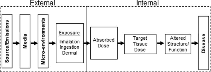
Conceptual Model for Exposure-related Disease. External and internal refer to the human body. (Adapted from Fig 2.12 of Maxwell, 2014⁷¹)

Environmental health scientists often try to examine the entire chain of causation illustrated in Figure 1 as improved understanding of that chain can assist the design of both epidemiologic studies and public health actions. But it is important to note that determining whether a specific intervention causally affects a disease may not depend on the target tissue dose, although the latter can help in understanding the results. For example, suppose the question of interest is whether reducing average ambient air concentrations of a toxicant has an effect on a health outcome of individuals. As an extreme example, suppose this was studied in a population where everyone stayed indoors and buildings possessed filters that prevented personal exposure to the ambient toxicant. The valid answer to this question is that reducing ambient concentration has no effect here (even if in unprotected populations the answer were different). Measurement of personal exposure (or, if possible, target tissue dose) would help in understanding this result. This is similar to the toxicologic issue of understanding differences between the results of whole animal and in vitro studies. A compound that is neurotoxic in an in vitro study may show no effect in an in vivo study because the compound is not absorbed or is eliminated by a first pass effect in the liver (when administered orally) or cannot cross the blood–brain barrier. Nevertheless, both causal questions are valid.

Alternatively, suppose that the question is defined as whether personal exposure to air pollution affects the health of an individual. In this case, the error in using ambient monitor-based exposure assessment as a proxy to estimate individual exposures is a concern. Our intent in this paper is to focus on situations where personal exposure or target tissue dose are of interest. Causal questions about target tissue dose also raise issues about what constitutes “well-defined interventions,”^5,6 which we do not have space here to discuss in detail. However, while directly changing the concentrations of a toxicant at a target tissue may be difficult outside of a laboratory, it can be conceptualized as an epidemiologic intervention. In addition, the arguments we put forward here also apply if we only consider exposure measures starting at the level of external personal exposure.

A measure of absorbed dose—e.g. a biomarker like toxicant concentration in blood—is often as close as an epidemiologist can get to the target tissue dose and can be a good proxy for it. In general we expect that proxy measures more removed from the target tissue dose will have more measurement error relative to the target tissue dose. For example, polybrominated diphenyl ethers (PBDEs) are flame-retardants commonly found in indoor dust. We could measure PBDE concentrations in a study participant’s serum (absorbed dose). Or we could measure PBDEs more distally, such as amounts in handwipes collected from participant’s hands (personal exposure) or amounts in dust samples from the participant’s living room (microenvironment). As an estimate of PBDE concentration at a target tissue, these latter options are further removed than serum concentration and thus have more measurement error relative to the target tissue dose because of differences between people in how house dust comes into contact with the participant, and in how what reaches the participant gets into the blood. Similarly, a personal air monitor on a study participant (personal exposure) will be a more accurate exposure estimate for that person’s air pollutant exposures than will air sampling from their bedroom (microenvironment) or predictions of ambient concentrations at the person’s residence based on concentrations at the nearest ambient monitor to their residence or a spatiotemporal model (media). We know people don’t spend all their time at home: the more time spent away from home, the less well the residential ambient pollution prediction will reflect the individual’s true personal exposure. The amount of time any individual spends indoors vs. outdoors at home may vary and outdoor air pollutant concentrations don’t perfectly predict indoor concentrations.

The effects of exposure measurement error on effect estimates differ depending on the specific error structure, and understanding error structures is an important research question. For non-differential measurement error the main types of structure are Berksonian and classical, or slight variations/mixtures of those. Berksonian error will decrease the precision of an estimate, but will not (on its own) bias the effect estimate. Classical error, in contrast, is expected to bias the effect estimate towards the null, which is a primary concern about measurement error—one that pervades environmental epidemiology. (There are notable exceptions of other error structures for which non-differential measurement error can bias away from the null, e.g.^7–10). In fact, because of this, it has been noted in the occupational literature that there are times when group measures may have advantages over individual measures because the error structure tends more towards Berksonian than classical.^11,12 A similar phenomenon may occur when using more smoothed area air pollution measures. While there are methods to mitigate bias towards the null,¹³ under ideal circumstances, a more personal exposure measurement would be preferred because a more accurate target tissue dose representation implies a stronger and more accurate effect estimate.^14–17 The problem lies in the fact that circumstances are often far from ideal.

It is important to note that in what follows we are not discussing purely ecologic studies where all variables—outcome, exposure, confounders, effect measure modifiers—are measured at the group level. Rather we mean individual-level studies that use exposure measures that are more (or less) removed from the individual target tissue dose.

Confounding bias

Exposure measurement error in environmental epidemiology studies, and attendant bias to the null, is an important concern, but it is not the only one. At least as important, and in some cases more so, is the concern of confounding bias. The starkest description of ideal circumstances with respect to this is one in which individual exposure is randomized, as in clinical drug trials. In environmental health this is rarely, if ever, possible. Therefore, one has to consider, for example in the case of absorbed dose, how the toxicant came to be at the concentration measured in the blood. This is dependent on individual characteristics such as toxicant pharmacokinetics and, of course, the level of the individual’s exposure to the toxicant in the environment, but that may depend on behaviors of the individual. These factors (covariates) then can introduce confounding if they are related to the health outcome (other than through the exposure of interest) as illustrated in the directed acyclic graph (DAG)^5,18,19 of Figure 2. Although one can try to control for such confounding, this can be a difficult task and in any epidemiology study the specter of residual or unmeasured confounding is very hard to avoid. We argue that while estimating the target tissue dose with measures that are more removed from the individual increases the error in estimating that target tissue dose, it may have the important advantage of decreasing sources of potential confounding bias that otherwise may be difficult to control. This potential tradeoff needs to be carefully considered.

Figure 2.

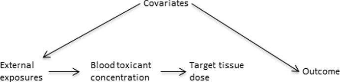
Causal diagram showing confounding of a toxicant (either measured in blood or in the target tissue)-outcome association by other covariates, drawn under the null assumption of no association between the target tissue dose and the outcome.

Potential epidemiologic advantages of proxy measures

To illustrate the potential advantages of more proxy exposure estimates consider the case of ambient air pollution. A large literature on the relation between aspects of ambient air pollution and different health outcomes exists that relies on estimates of exposure derived from area air monitors or satellite imaging.^20–23 For example, investigators use concentrations at the closest monitor (or some weighted average) to an individual’s residence, or spatiotemporal models that incorporate monitor data and spatially and temporally varying factors—e.g. traffic patterns, meteorological factors, land use characteristics—to predict outdoor ambient pollutant concentrations at the individual’s residence in a given time window. These methods have been used to examine the effects of air pollution on many different health outcomes including cardiovascular,²⁴ respiratory,^25–27 and neurological effects,^28,29 as well as overall mortality.^30–32

The DAG of Figure 3A depicts a structure that assumes that the effect of exposure to ambient air pollution goes through personal exposure. In this way the ambient air pollution prediction is a proxy measure for personal air pollution exposure and target tissue dose. Note that personal behavior differences affect personal exposure assessments directly, but they do not affect the ambient concentration prediction. In the DAG of figure 3A, personal behavior differences (one could add personal biological characteristics like genetics here as well—either pointing into personal exposure or target tissue dose) introduce confounding to the association between personal exposure and the outcome (note that the direct arrow from personal behavior to outcome could be replaced with other statistical paths connecting the two), but not to the association between the ambient concentration prediction and the health outcome.⁵ In fact, in the DAG of figure 3A as drawn, the ambient concentration prediction is an instrumental variable (IV) for personal pollutant exposure, because it fulfills the three conditions for an IV^33,34: i) ambient concentration prediction is associated with personal air pollutant exposure, ii) ambient concentration prediction does not cause the outcome except through personal air pollutant exposure, and iii) ambient concentration prediction does not share any causes with the outcome. As such, the ambient concentration prediction avoids confounding by measured or unmeasured (even unknown) variables like the personal behaviors indicated in the figure that confound the personal exposure–health outcome association.^33,34

Figure 3.

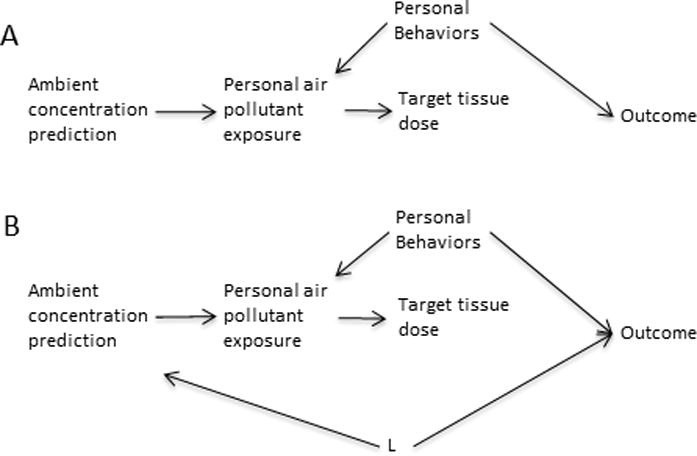
A) Causal diagram showing a personal air pollutant exposure measure acting as a collider between an ambient concentration prediction and an outcome, drawn under the null assumption of no association between personal air pollutant exposure (presumably acting via effects on a target tissue) and the outcome. Under this causal diagram, the personal behavior variables do not introduce confounding of the ambient concentration-outcome association. B) The same as in A with the addition of an illustration of the structure needed for variables (L) to introduce confounding of the ambient air pollutant prediction-outcome association.

The DAG of Figure 3A, however, is clearly over-simplified. It is possible that there could be confounding of the association between the ambient concentration prediction and the outcome by other variables (L) (Figure 3B), violating the third requirement of an IV (note that if all possible L could be fully controlled, then the ambient concentration prediction could still be an IV conditional on controlling those L variables). These L variables should be predictors of ambient air pollution like socioeconomic status (SES) (potentially both individual and area), urbanicity, population density, and meteorological variables.^35–39 SES factors can affect where a person lives, which can be related to many health outcomes; urbanicity and population density could be related to case ascertainment issues; and meteorological factors at least in some cases could be related to health outcomes.^40,41 However, these L variables also introduce confounding to the personal exposure-outcome association (Figure 3B). Thus, the set of possible confounding variables for the ambient concentration estimation cannot be larger than that for personal exposure. The magnitude of, and ability to control confounding by L of the ambient estimate vs. confounding of the personal exposure estimate by personal behavior and L is hard to gauge and needs to be evaluated in any study setting. However, in the case of ambient air pollution, and perhaps in other exposure model settings, we hypothesize that the predictors of the proxy exposure estimate may be better understood and controlled than individual behavioral predictors of personal exposure. (However, one potential problem is that group-level exposure variables have the potential to introduce aspects of ecologic bias, even in otherwise individual-level studies^7,42,43).

Similarly, physiologic factors may sometimes confound associations between biomarkers of exposure and health outcomes. For example, it has been suggested that much of the association between maternal or cord plasma perfluoroalkyl substances (PFAS) and birthweight can be explained by confounding by glomerular filtration rate (GFR)⁴⁴—that is, that differences in GFR and the size of the developing fetus (and eventually birthweight) are both related to some maternal factors. Thus, because differences in GFR affect the concentration of plasma PFAS, the PFAS-birthweight association is confounded as illustrated in figure 4. In some settings it is possible to develop models of external exposures to PFAS, for example using data on contamination of drinking water sources in the mid-Ohio valley region.⁴⁵ Using such a model of external PFAS exposures as a proxy for plasma PFAS would avoid the confounding from maternal factors that affect GFR (as well as confounding by personal behavior differences as described above) (Figure 4). While one could avoid this by using pre-pregnancy samples or controlling GFR, these data can be hard to get and in some studies, e.g. of insidious onset diseases, one may not know when “before” the disease is.

Figure 4.

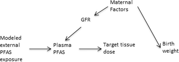
A) Causal diagram showing an example of a structure of confounding of the plasma perfluoroalkyl substances (PFAS)-outcome association by physiological factors under the null assumption of no PFAS-outcome association. Here effects of maternal physiological factors on glomerular filtration rate (GFR), which affects the measured concentration of PFAS in maternal blood during pregnancy, results in confounding of the PFAS-birthweight association. A modeled estimate of external PFAS exposure avoids confounding by the physiological factors because the plasma PFAS concentration acts as a collider between the modeled exposure and the physiological factors.

This general concept of the use of more proxy exposure estimates to avoid confounding in analyses of less proxy measures is precisely why one does intention-to-treat analyses in randomized control trials.⁵ Assignment to a drug treatment arm is a more proxy exposure estimate than is actual medications taken or internal dose of the medication because not all people assigned to the drug take it as the investigators intend (and possibly those in the control arm could get access to the drug by other means). While using the actual medications taken or a measure of internal dose would provide a more accurate indication of the exposure to the drug, analyses with those exposures would be subject to confounding by all the factors that predict whether the drug is taken and how it is absorbed. A similar concept of using more proxy exposure measures as IVs for personal exposure has been discussed in the occupational literature. For example, it has been pointed out that if individual personal exposure measurements are made among workers in a particular group (e.g. those in a particular job), then the average of the individual measures, under some conditions, can act like an IV for individual-level exposure.⁴⁶ The reason this approach only works under some conditions is that the group average exposure violates one of the three requirements for an IV. If the more proxy exposure estimate is based on averages of individual exposure measures, then the variables that cause confounding of the individual exposure measure-outcome association can also introduce confounding of the group average-outcome association, violating the third condition for an IV listed above. In this case the advantage of using the more proxy exposure estimate is diminished, as it would also require control of the variables that could confound the more personal exposure measure, although the degree to which the IV condition is violated diminishes with larger group sizes.⁴⁶ This is not a problem if individual characteristics do not influence the more proxy estimate, as in our example of ambient air pollution predictions. A slightly different issue, but one that shares some similarities, is how under some conditions gene-only models often more reliably indicate the presence—if not precise magnitude—of a gene–environment interaction than a model with an environmental exposure and gene-by-environment interaction term, in part because only including the gene term avoids potential confounding bias from variables that confound the environmental exposure–outcome association.^47,48

Examples

If more proxy exposure estimates avoid confounding from personal factors that affect personal exposure (or target tissue dose) measures, then effect estimates for those more proxy measures should not be affected by adjustment for the personal factors, although even in the complete absence of confounding some small change will likely be present just from statistical fluctuation. The examples in Table 1 are consistent with our argument that more proxy measures are less susceptible to confounding by personal factors, but they cannot prove that. If the personal factor does not confound the association with the personal exposure (or target tissue dose) measure (perhaps because it is not related to the personal exposure or because adjustment for other factors sufficiently adjusts for the personal factor in question), then showing that it does not confound a more proxy measure does not inform our argument. In the traffic pollution study in table 1⁴⁹ we assume, for example, that playing sports could affect personal traffic pollution exposure (perhaps related to location) as well as atrial fibrillation (through exercise), and thus confound the association with personal exposure. If so, the lack of change in the effect estimate for the model-based traffic pollution estimate argues for our point, but not if the confounding at the personal level is minimal (maybe because there wasn’t an association between playing sports and traffic pollution exposure). To empirically address our hypothesis, what is needed are studies that estimate exposure with both a more proxy and a personal exposure measure and collect data on a personal variable that introduces confounding of the personal exposure measure-outcome association.

Table 1.

Examples of more proxy exposure measure effect estimates before and after additional adjustment for personal factors.

		Effect estimate (95% confidence interval)
Reference	Details	Before	After
Ritz et al., 200767	Exposure: Ambient CO (nearest monitor approach) Outcome: Pre-term birth Contrast: 1st trimester top quartile vs bottom quartile Base adjustment: Birth season, parity, mother’s age, race, and education Additional personal factor adjustments: active and passive smoking, marital status, and alcohol use during pregnancy	OR: 1.21 (0.89–1.65)	OR: 1.21 (0.88–1.65)
Ritz et al., 200767	Exposure: Ambient PM2.5 (nearest monitor approach) Outcome: Pre-term birth Contrast: 1st trimester top tertile vs bottom tertile Base adjustment: Birth season, parity, mother’s age, race, and education Additional personal factor adjustments: active and passive smoking, marital status, and alcohol use during pregnancy	OR: 1.27 (0.99–1.64)	OR: 1.29 (1.00–1.67)
Monrad et al. 201649	Exposure: Traffic-related pollution (dispersion model) Outcome: Atrial fibrillation Contrast: per 10μg/m3 10-year mean NO2 Base adjustment: Age Additional personal factor adjustments: Sex, body mass index, waist circumference, smoking status, smoking duration, smoking intensity, intake of alcohol, sport during leisure time, length of school attendance, area level socioeconomic position and calendar year	IRR: 1.08 (1.02–1.15)	IRR: 1.08 (1.01–1.14)
Monrad et al. 201649	Exposure: Traffic-related pollution (dispersion model) Outcome: Atrial fibrillation Contrast: per 10μg/m3 10-year mean NOX Base adjustment: Age Additional personal factor adjustments: Sex, body mass index, waist circumference, smoking status, smoking duration, smoking intensity, intake of alcohol, sport during leisure time, length of school attendance, area level socioeconomic position and calendar year	IRR: 1.17 (1.03–1.32)	IRR: 1.16 (1.02–1.32)
Aschengrau et al., 200968	Exposure: PCE; modeled from piping in water distribution system Outcome: Congenital anomalies Contrast: In utero exposure >1980 action level of 40μg/L vs. below Base adjustment: None Additional personal factor adjustments: Parental agesa	OR: 1.4 (0.9–2.2)	OR: 1.4 (0.9–2.2)
Hart et al., 201516b	Exposure: PM2.5; spatiotemporal model Outcome: Mortality Contrast: per 10μg/m3 Base adjustment: age, race, region, year, season, census tract median family income and median house value, education level, parents’ occupation, marital status, and husband’s education Additional personal factor adjustments: smoking (both never, past, current and packyears)	HR: 1.17 (1.09–1.27)	HR: 1.19 (1.10–1.29)

Abbreviations: CO: Carbon monoxide; OR: Odds ratio; PM_2.5: Particulate matter <2.5 micrometers in diameter; NO₂: Nitrogen dioxide; IRR: Incidence rate ratio; PCE: Tetrachloroethylene; HR: Hazard Ratio.

^aSimilar lack of change of effect estimates seen after adjustment for many other personal factors was also reported, but data not shown; this has also been noted by this group in other studies of theirs as well.^69,70

^bResults are from models with slightly different variable sets than in the original paper and were provided by Dr. Jaime Hart.

Reverse causation

An additional benefit of less-individual based exposure estimates is that they can avoid biases from reverse causation. In many cases use of a biosample to assess personal exposure to a contaminant can be compromised by unrecognized effects of the outcome (or antecedents of the outcome) on the measurement of the toxicant in the biosample. An interesting potential case of reverse causation is PBDEs and hyperthyroidism in cats. Prevalence of feline hyperthyroidism has increased over the last several decades, making it a common disease of older cats.⁵⁰ Risk factors include certain kinds of diet and living indoors; endocrine disruption by environmental chemicals, such as PBDEs, has also been hypothesized. Cats have higher levels of PBDEs than humans, potentially due to grooming behavior (e.g.,⁵¹) since PBDEs are found in house dust. PBDEs have been associated with altered thyroid hormone levels in both laboratory animals and humans (e.g.,^52,53). Of six small cross-sectional studies of PBDEs and feline hyperthyroidism, two reported associations between PBDE concentrations in blood (on a lipid weight basis) and hyperthyroidism.^51,54–58 However, feline hyperthyroidism causes substantial weight loss. As PBDEs are lipophilic, weight loss will tend to increase concentrations of such compounds in body lipids, including blood lipid. Indeed, a few studies report elevated concentrations of other lipophilic compounds. Thus the reported associations may be at least partly due to reverse causation (Figure 5).⁵⁴ Use of dust as a proxy exposure measure has the potential of mitigating the reverse causation because if reverse causation accounts for the association between blood PBDE and feline hyperthyroidism, then no association between dust concentrations and hyperthyroidism would be seen (Figure 5).

Figure 5.

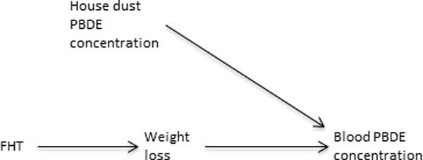
Causal diagram illustrating how feline hyperthyroidism (FHT) may be associated with serum polybrominated diphenylethers (PBDEs) via reverse causation. FHT causes weight loss that increases concentrations of PBDEs in body fat and blood lipid. House dust (and diet, not shown) are the source of PBDE exposure and not related to FHT under the null assumption of no causal association between the two because blood PBDE concentration is a collider between them.

Conclusions

In summary, there may often be a tradeoff between exposure measurement error and potential confounding as exposure estimates are more removed from the individual. Personal behaviors and individual physiologic factors can confound associations between biosample measures and health outcomes; an individual’s metabolism shouldn’t confound microenvironment measurement–outcome associations, but individual behaviors could (although likely less than with a biomarker); neither should confound associations with estimates based on sources and emissions or larger scale media. We hypothesize that the factors introducing confounding to an association with a more proxy exposure estimate are often fewer and more easily identifiable than those that could do so for an association with a personal exposure measurement. When using a more proxy exposure estimate, personal behaviors or pre-clinical aspects of the outcome under study are not a concern because actual personal exposure is a collider between the more proxy estimate and factors that cause confounding or reverse causation of personal exposure-outcome associations. Factors that can confound a personal exposure–outcome association can often be extremely hard to completely identify, let alone condition out analytically. Furthermore, while some variables could still introduce confounding to an association with a more proxy exposure estimate, for example SES factors, these variables would still be of concern in an analysis with a personal exposure measure. It is also important to note that for relatively time-invariant covariates like SES factors, if specific time windows of exposure for associations with an outcome are found, this can rule out confounding by time-invariant variables based on negative control exposures principles.^29,59–61 Although there are methods that have been proposed to account for unmeasured confounding,^62–64 they necessarily make assumptions about the structure of the unmeasured (possibly unknown) confounding. Thus, the possibility of simply eliminating some possible confounding may sometimes be preferable.

The critical aspect of a more proxy exposure estimate that allows its use to avoid much confounding and reverse causation that can affect more personal exposure measurements is that the factors used in creating the exposure estimate, and the distribution of the exposure in the environment, are unrelated to individual behaviors or characteristics of those in the study population. It is, however, critical that the exposure estimate be reasonably good or bias to the null from exposure misclassification could be so pronounced as to obscure true associations. An association with a more proxy measure is likely to be biased to the null compared with the true personal exposure–outcome association. So while the proxy may effectively indicate the presence of a personal exposure–outcome association, it likely does not accurately reflect its magnitude. Thus, studies to understand how well a proxy exposure estimate predicts actual personal exposures are critical. With such data one can use established methods to correct for bias to the null from measurement error.^12,13,65,66 The fact that this can be done is another argument for using more proxy exposure estimates: the drawback of bias to the null from exposure measurement error may be more easily addressed than the drawback with more personal exposure measures of needing to control for additional confounding or reverse causation biases that may not even be recognized. Furthermore, with the more proxy exposure estimate there is the possibility of using the correlation with more personal exposure in IV analyses.^29,30 In addition, in many settings it is not feasible to make individual measurements on everyone.

We believe that more research is needed into the degree of bias to the null with measurement error in different settings and on the degree of confounding introduced by personal exposure measures. Comparisons of the magnitude of these two effects would be a useful line of research. However, the potential value of more proxy exposure estimates to avoid important sources of confounding—even some of which we are unaware—should not be overlooked when deciding how to handle exposure assessment for a study.

References

- 1.Koehler KA, Peters TM. New Methods for Personal Exposure Monitoring for Airborne Particles. Curr Environ Health Rep. 2015;2(4):399–411. doi: 10.1007/s40572-015-0070-z. [DOI] [PMC free article] [PubMed] [Google Scholar]
- 2.Hammel SC, Hoffman K, Webster TF, Anderson KA, Stapleton HM. Measuring Personal Exposure to Organophosphate Flame Retardants Using Silicone Wristbands and Hand Wipes. Environ Sci Technol. 2016;50(8):4483–91. doi: 10.1021/acs.est.6b00030. [DOI] [PMC free article] [PubMed] [Google Scholar]
- 3.O’Connell SG, Kincl LD, Anderson KA. Silicone wristbands as personal passive samplers. Environ Sci Technol. 2014;48(6):3327–35. doi: 10.1021/es405022f. [DOI] [PMC free article] [PubMed] [Google Scholar]
- 4.Centers for Disease Control and Prevention. Services USDoHaH. Atlanta, GA: 2015. Fourth Report on Human Exposure to Environmental Chemicals, Updated Tables February 2015. [Google Scholar]
- 5.Hernan MA, Robins JM. Causal Inference. Abingdon, UK: Chapman & Hall/CRC; 2015. [Google Scholar]
- 6.Vandenbroucke JP, Broadbent A, Pearce N. Causality and causal inference in epidemiology: the need for a pluralistic approach. Int J Epidemiol. 2016 doi: 10.1093/ije/dyv341. [DOI] [PMC free article] [PubMed] [Google Scholar]
- 7.Webster T. Commentary: does the spectre of ecologic bias haunt epidemiology? Int J Epidemiol. 2002;31(1):161–2. doi: 10.1093/ije/31.1.161. [DOI] [PubMed] [Google Scholar]
- 8.Webster TF. Bias magnification in ecologic studies: a methodological investigation. Environ Health. 2007;6:17. doi: 10.1186/1476-069X-6-17. [DOI] [PMC free article] [PubMed] [Google Scholar]
- 9.Brenner H, Savitz DA, Jockel KH, Greenland S. Effects of nondifferential exposure misclassification in ecologic studies. Am J Epidemiol. 1992;135(1):85–95. doi: 10.1093/oxfordjournals.aje.a116205. [DOI] [PubMed] [Google Scholar]
- 10.Berkson J. Are There Two Regressions? Journal of the American Statistical Association. 1950;45(250):164–180. [Google Scholar]
- 11.Tielemans E, Kupper LL, Kromhout H, Heederik D, Houba R. Individual-based and group-based occupational exposure assessment: some equations to evaluate different strategies. Ann Occup Hyg. 1998;42(2):115–9. doi: 10.1016/s0003-4878(97)00051-3. [DOI] [PubMed] [Google Scholar]
- 12.Kim HM, Richardson D, Loomis D, Van Tongeren M, Burstyn I. Bias in the estimation of exposure effects with individual- or group-based exposure assessment. J Expo Sci Environ Epidemiol. 2011;21(2):212–21. doi: 10.1038/jes.2009.74. [DOI] [PubMed] [Google Scholar]
- 13.Rosner B, Spiegelman D, Willett WC. Correction of logistic regression relative risk estimates and confidence intervals for random within-person measurement error. Am J Epidemiol. 1992;136(11):1400–13. doi: 10.1093/oxfordjournals.aje.a116453. [DOI] [PubMed] [Google Scholar]
- 14.Kioumourtzoglou M, Spiegelman D, Szpiro A, Sheppard L, Kaufman J, Yanosky J, Williams R, Laden F, Hong B, Suh H. Exposure measurement error in PM2.5 health effects studies: A pooled analysis of eight personal exposure validation studies. Environ Heal. 2014;13(1):2. doi: 10.1186/1476-069X-13-2. [DOI] [PMC free article] [PubMed] [Google Scholar]
- 15.Setton E, Marshall JD, Brauer M, Lundquist KR, Hystad P, Keller P, Cloutier-Fisher D. The impact of daily mobility on exposure to traffic-related air pollution and health effect estimates. J Expo Sci Environ Epidemiol. 2011;21(1):42–8. doi: 10.1038/jes.2010.14. [DOI] [PubMed] [Google Scholar]
- 16.Hart J, Liao X, Hong B, Puett R, Yanosky J, Suh H, Kioumourtzoglou M, Spiegelman D, Laden F. The association of long-term exposure to PM2.5 on all-cause mortality in the Nurses’ Health Study and the impact of measurement-error correction. Environ Health. 2015;14:38. doi: 10.1186/s12940-015-0027-6. [DOI] [PMC free article] [PubMed] [Google Scholar]
- 17.Watkins DJ, McClean MD, Fraser AJ, Weinberg J, Stapleton HM, Sjodin A, Webster TF. Exposure to PBDEs in the office environment: evaluating the relationships between dust, handwipes, and serum. Environ Health Perspect. 2011;119(9):1247–52. doi: 10.1289/ehp.1003271. [DOI] [PMC free article] [PubMed] [Google Scholar]
- 18.Greenland S, Pearl J, Robins JM. Causal diagrams for epidemiologic research. Epidemiology. 1999;10(1):37–48. [PubMed] [Google Scholar]
- 19.Pearl J. Causal diagrams for empirical research. Biometrika. 1995;82:669–88. [Google Scholar]
- 20.Hoek G, Beelen R, de Hoogh K, Vienneau D, Gulliver J, Fischer P, Briggs D. A review of land-use regression models to assess spatial variation of outdoor air pollution. Atmos Environ. 2008;42(33):7561–7578. [Google Scholar]
- 21.Jerrett M, Arain A, Kanaroglou P, Beckerman B, Potoglou D, Sahsuvaroglu T, Morrison J, Giovis C. A review and evaluation of intraurban air pollution exposure models. J Expo Anal Environ Epidemiol. 2005;15(2):185–204. doi: 10.1038/sj.jea.7500388. [DOI] [PubMed] [Google Scholar]
- 22.Kloog I, Nordio F, Coull BA, Schwartz J. Incorporating local land use regression and satellite aerosol optical depth in a hybrid model of spatiotemporal PM2.5 exposures in the Mid-Atlantic states. Environ Sci Technol. 2012;46(21):11913–21. doi: 10.1021/es302673e. [DOI] [PMC free article] [PubMed] [Google Scholar]
- 23.Yanosky JD, Paciorek CJ, Laden F, Hart JE, Puett RC, Liao D, Suh HH. Spatio-temporal modeling of particulate air pollution in the conterminous United States using geographic and meteorological predictors. Environ Health. 2014;13:63. doi: 10.1186/1476-069X-13-63. [DOI] [PMC free article] [PubMed] [Google Scholar]
- 24.Brook RD, Rajagopalan S, Pope CA, 3rd, Brook JR, Bhatnagar A, Diez-Roux AV, Holguin F, Hong Y, Luepker RV, Mittleman MA, Peters A, Siscovick D, Smith SC, Jr, Whitsel L, Kaufman JD. Particulate matter air pollution and cardiovascular disease: An update to the scientific statement from the American Heart Association. Circulation. 2010;121(21):2331–78. doi: 10.1161/CIR.0b013e3181dbece1. Epub 2010 May 10. [DOI] [PubMed] [Google Scholar]
- 25.Hoek G, Krishnan RM, Beelen R, Peters A, Ostro B, Brunekreef B, Kaufman JD. Long-term air pollution exposure and cardio- respiratory mortality: a review. Environ Health. 2013;12(1):43. doi: 10.1186/1476-069X-12-43. [DOI] [PMC free article] [PubMed] [Google Scholar]
- 26.Atkinson RW, Anderson HR, Sunyer J, Ayres J, Baccini M, Vonk JM, Boumghar A, Forastiere F, Forsberg B, Touloumi G, Schwartz J, Katsouyanni K. Acute effects of particulate air pollution on respiratory admissions: results from APHEA 2 project. Air Pollution and Health: a European Approach. Am J Respir Crit Care Med. 2001;164(10 Pt 1):1860–6. doi: 10.1164/ajrccm.164.10.2010138. [DOI] [PubMed] [Google Scholar]
- 27.Dominici F, Peng RD, Bell ML, Pham L, McDermott A, Zeger SL, Samet JM. Fine particulate air pollution and hospital admission for cardiovascular and respiratory diseases. JAMA. 2006;295(10):1127–34. doi: 10.1001/jama.295.10.1127. [DOI] [PMC free article] [PubMed] [Google Scholar]
- 28.Block M, Elder A, Auten R, Chen H, Chen J, Cory-Slechta D, Costa D, Diaz-Sanchez D, Dorman D, Gold D, Gray K, Jeng H, Kaufman J, Kleinman M, Kirshner A, Lawler C, Miller D, Nadadur S, Ritz B, Semmens E, Tonelli L, Veronesi B, Wright R, Wright R. The outdoor air pollution and brain health workshop. Neurotoxicology. 2012;33(5):972–984. doi: 10.1016/j.neuro.2012.08.014. [DOI] [PMC free article] [PubMed] [Google Scholar]
- 29.Weisskopf M, Kioumourtzoglou M-A, Roberts A. Air Pollution and Autism Spectrum Disorders: Causal or Confounded? Current Environmental Health Reports. 2015:1–10. doi: 10.1007/s40572-015-0073-9. [DOI] [PMC free article] [PubMed] [Google Scholar]
- 30.Beelen R, Hoek G, Raaschou-Nielsen O, Stafoggia M, Andersen ZJ, Weinmayr G, Hoffmann B, Wolf K, Samoli E, Fischer PH, Nieuwenhuijsen MJ, Xun WW, Katsouyanni K, Dimakopoulou K, Marcon A, Vartiainen E, Lanki T, Yli-Tuomi T, Oftedal B, Schwarze PE, Nafstad P, De Faire U, Pedersen NL, Ostenson CG, Fratiglioni L, Penell J, Korek M, Pershagen G, Eriksen KT, Overvad K, Sorensen M, Eeftens M, Peeters PH, Meliefste K, Wang M, Bueno-de-Mesquita HB, Sugiri D, Kramer U, Heinrich J, de Hoogh K, Key T, Peters A, Hampel R, Concin H, Nagel G, Jaensch A, Ineichen A, Tsai MY, Schaffner E, Probst-Hensch NM, Schindler C, Ragettli MS, Vilier A, Clavel-Chapelon F, Declercq C, Ricceri F, Sacerdote C, Galassi C, Migliore E, Ranzi A, Cesaroni G, Badaloni C, Forastiere F, Katsoulis M, Trichopoulou A, Keuken M, Jedynska A, Kooter IM, Kukkonen J, Sokhi RS, Vineis P, Brunekreef B. Natural-cause mortality and long-term exposure to particle components: an analysis of 19 European cohorts within the multi-center ESCAPE project. Environ Health Perspect. 2015;123(6):525–33. doi: 10.1289/ehp.1408095. [DOI] [PMC free article] [PubMed] [Google Scholar]
- 31.Dockery DW, Pope CA, 3rd, Xu X, Spengler JD, Ware JH, Fay ME, Ferris BG, Jr, Speizer FE. An association between air pollution and mortality in six U.S. cities. N Engl J Med. 1993;329(24):1753–9. doi: 10.1056/NEJM199312093292401. [DOI] [PubMed] [Google Scholar]
- 32.Kioumourtzoglou MA, Schwartz J, James P, Dominici F, Zanobetti A. PM2.5and mortality in 207 US cities: Modification by temperature and city characteristics. Epidemiology. 2015 doi: 10.1097/EDE.0000000000000422. [DOI] [PMC free article] [PubMed] [Google Scholar]
- 33.Hernan MA, Robins JM. Instruments for causal inference: an epidemiologist’s dream? Epidemiology. 2006;17(4):360–72. doi: 10.1097/01.ede.0000222409.00878.37. [DOI] [PubMed] [Google Scholar]
- 34.Greenland S. An introduction to instrumental variables for epidemiologists. Int J Epidemiol. 2000;29(4):722–9. doi: 10.1093/ije/29.4.722. [DOI] [PubMed] [Google Scholar]
- 35.Shmool JL, Kubzansky LD, Newman OD, Spengler J, Shepard P, Clougherty JE. Social stressors and air pollution across New York City communities: a spatial approach for assessing correlations among multiple exposures. Environ Health. 2014;13:91. doi: 10.1186/1476-069X-13-91. [DOI] [PMC free article] [PubMed] [Google Scholar]
- 36.Marshall JD, Brauer M, Frank LD. Healthy neighborhoods: walkability and air pollution. Environ Health Perspect. 2009;117(11):1752–9. doi: 10.1289/ehp.0900595. [DOI] [PMC free article] [PubMed] [Google Scholar]
- 37.Clark LP, Millet DB, Marshall JD. Air quality and urban form in U.S. urban areas: evidence from regulatory monitors. Environ Sci Technol. 2011;45(16):7028–35. doi: 10.1021/es2006786. [DOI] [PubMed] [Google Scholar]
- 38.Bell M, Ebisu K. Environmental inequality in exposures to airborne particulate matter components in the United States. Environ Health Perspect. 2012;120(12):1699–704. doi: 10.1289/ehp.1205201. [DOI] [PMC free article] [PubMed] [Google Scholar]
- 39.Seinfeld JH, Pandis SN. Atmospheric Chemistry and Physics: From Air Pollution to Climate Change. 2. Hoboken, NJ: John Wiley & Sons, Inc; 2006. [Google Scholar]
- 40.Basu R, Malig B. High ambient temperature and mortality in California: exploring the roles of age, disease, and mortality displacement. Environ Res. 2011;111(8):1286–92. doi: 10.1016/j.envres.2011.09.006. [DOI] [PubMed] [Google Scholar]
- 41.Strand LB, Barnett AG, Tong S. Maternal exposure to ambient temperature and the risks of preterm birth and stillbirth in Brisbane, Australia. Am J Epidemiol. 2012;175(2):99–107. doi: 10.1093/aje/kwr404. [DOI] [PubMed] [Google Scholar]
- 42.Webster T. Bias in Ecologic and Semi-individual Studies. Boston University School of Public Health; 2000. [Google Scholar]
- 43.Bjork J, Stromberg U. Effects of systematic exposure assessment errors in partially ecologic case-control studies. Int J Epidemiol. 2002;31(1):154–60. doi: 10.1093/ije/31.1.154. [DOI] [PubMed] [Google Scholar]
- 44.Verner MA, Loccisano AE, Morken NH, Yoon M, Wu H, McDougall R, Maisonet M, Marcus M, Kishi R, Miyashita C, Chen MH, Hsieh WS, Andersen ME, Clewell HJ, Longnecker MP. Associations of Perfluoroalkyl Substances (PFAS) with Lower Birth Weight: An Evaluation of Potential Confounding by Glomerular Filtration Rate Using a Physiologically Based Pharmacokinetic Model (PBPK) Environ Health Perspect. 2015;123(12):1317–24. doi: 10.1289/ehp.1408837. [DOI] [PMC free article] [PubMed] [Google Scholar]
- 45.Shin HM, Vieira VM, Ryan PB, Steenland K, Bartell SM. Retrospective exposure estimation and predicted versus observed serum perfluorooctanoic acid concentrations for participants in the C8 Health Project. Environ Health Perspect. 2011;119(12):1760–5. doi: 10.1289/ehp.1103729. [DOI] [PMC free article] [PubMed] [Google Scholar]
- 46.Batistatou E, McNamee R. Instrumental variables vs grouping approach for reducing bias due to measurement error. Int J Biostat. 2008;4(1) doi: 10.2202/1557-4679.1087. Article 8. [DOI] [PubMed] [Google Scholar]
- 47.Burstyn I, Kim HM, Yasui Y, Cherry NM. The virtues of a deliberately mis-specified disease model in demonstrating a gene-environment interaction. Occup Environ Med. 2009;66(6):374–80. doi: 10.1136/oem.2008.039081. [DOI] [PubMed] [Google Scholar]
- 48.Luo H, Burstyn I, Gustafson P. Investigations of gene-disease associations: costs and benefits of environmental data. Epidemiology. 2013;24(4):562–8. doi: 10.1097/EDE.0b013e3182944dd5. [DOI] [PubMed] [Google Scholar]
- 49.Monrad M, Sajadieh A, Christensen JS, Ketzel M, Raaschou-Nielsen O, Tjonneland A, Overvad K, Loft S, Sorensen M. Long-Term Exposure to Traffic-Related Air Pollution and Risk of Incident Atrial Fibrillation: A Cohort Study. Environ Health Perspect. 2016 doi: 10.1289/EHP392. [DOI] [PMC free article] [PubMed] [Google Scholar]
- 50.Peterson M. Hyperthyroidism in cats: what’s causing this epidemic of thyroid disease and can we prevent it? J Feline Med Surg. 2012;14(11):804–18. doi: 10.1177/1098612X12464462. [DOI] [PMC free article] [PubMed] [Google Scholar]
- 51.Dye JA, Venier M, Zhu L, Ward CR, Hites RA, Birnbaum LS. Elevated PBDE levels in pet cats: sentinels for humans? Environ Sci Technol. 2007;41(18):6350–6. doi: 10.1021/es0708159. [DOI] [PubMed] [Google Scholar]
- 52.Makey CM, McClean MD, Braverman LE, Pearce EN, He XM, Sjodin A, Weinberg JM, Webster TF. Polybrominated Diphenyl Ether Exposure and Thyroid Function Tests in North American Adults. Environ Health Perspect. 2016;124(4):420–5. doi: 10.1289/ehp.1509755. [DOI] [PMC free article] [PubMed] [Google Scholar]
- 53.Chevrier J. Invited commentary: Maternal plasma polybrominated diphenyl ethers and thyroid hormones–challenges and opportunities. Am J Epidemiol. 2013;178(5):714–9. doi: 10.1093/aje/kwt138. [DOI] [PMC free article] [PubMed] [Google Scholar]
- 54.Guo W, Gardner S, Yen S, Petreas M, Park JS. Temporal Changes of PBDE Levels in California House Cats and a Link to Cat Hyperthyroidism. Environ Sci Technol. 2016;50(3):1510–8. doi: 10.1021/acs.est.5b04252. [DOI] [PubMed] [Google Scholar]
- 55.Guo W, Park JS, Wang Y, Gardner S, Baek C, Petreas M, Hooper K. High polybrominated diphenyl ether levels in California house cats: house dust a primary source? Environ Toxicol Chem. 2012;31(2):301–6. doi: 10.1002/etc.1700. [DOI] [PubMed] [Google Scholar]
- 56.Mensching DA, Slater M, Scott JW, Ferguson DC, Beasley VR. The feline thyroid gland: a model for endocrine disruption by polybrominated diphenyl ethers (PBDEs)? J Toxicol Environ Health A. 2012;75(4):201–12. doi: 10.1080/15287394.2012.652054. [DOI] [PubMed] [Google Scholar]
- 57.Norrgran J, Jones B, Bignert A, Athanassiadis I, Bergman A. Higher PBDE serum concentrations may be associated with feline hyperthyroidism in Swedish cats. Environ Sci Technol. 2015;49(8):5107–14. doi: 10.1021/acs.est.5b00234. [DOI] [PubMed] [Google Scholar]
- 58.Chow K, Hearn LK, Zuber M, Beatty JA, Mueller JF, Barrs VR. Evaluation of polybrominated diphenyl ethers (PBDEs) in matched cat sera and house dust samples: investigation of a potential link between PBDEs and spontaneous feline hyperthyroidism. Environ Res. 2015;136:173–9. doi: 10.1016/j.envres.2014.09.027. [DOI] [PubMed] [Google Scholar]
- 59.Lipsitch M, Tchetgen Tchetgen E, Cohen T. Negative controls: a tool for detecting confounding and bias in observational studies. Epidemiology. 2010;21(3):383–8. doi: 10.1097/EDE.0b013e3181d61eeb. [DOI] [PMC free article] [PubMed] [Google Scholar]
- 60.Weisskopf MG, Tchetgen Tchetgen EJ, Raz R. Commentary: On the Use of Imperfect Negative Control Exposures in Epidemiologic Studies. Epidemiology. 2016;27(3):365–7. doi: 10.1097/EDE.0000000000000454. [DOI] [PubMed] [Google Scholar]
- 61.Flanders WD, Klein M, Darrow LA, Strickland MJ, Sarnat SE, Sarnat JA, Waller LA, Winquist A, Tolbert PE. A method for detection of residual confounding in time-series and other observational studies. Epidemiology. 2011;22(1):59–67. doi: 10.1097/EDE.0b013e3181fdcabe. [DOI] [PMC free article] [PubMed] [Google Scholar]
- 62.McCandless LC, Gustafson P, Levy A. Bayesian sensitivity analysis for unmeasured confounding in observational studies. Stat Med. 2007;26(11):2331–47. doi: 10.1002/sim.2711. [DOI] [PubMed] [Google Scholar]
- 63.McCandless LC, Gustafson P, Levy AR. A sensitivity analysis using information about measured confounders yielded improved uncertainty assessments for unmeasured confounding. J Clin Epidemiol. 2008;61(3):247–55. doi: 10.1016/j.jclinepi.2007.05.006. [DOI] [PubMed] [Google Scholar]
- 64.Gustafson P, McCandless LC, Levy AR, Richardson S. Simplified Bayesian sensitivity analysis for mismeasured and unobserved confounders. Biometrics. 2010;66(4):1129–37. doi: 10.1111/j.1541-0420.2009.01377.x. [DOI] [PubMed] [Google Scholar]
- 65.Preller L, Kromhout H, Heederik D, Tielen MJ. Modeling long-term average exposure in occupational exposure-response analysis. Scand J Work Environ Health. 1995;21(6):504–12. doi: 10.5271/sjweh.67. [DOI] [PubMed] [Google Scholar]
- 66.Xing L, Burstyn I, Richardson DB, Gustafson P. A comparison of Bayesian hierarchical modeling with group-based exposure assessment in occupational epidemiology. Stat Med. 2013;32(21):3686–99. doi: 10.1002/sim.5791. [DOI] [PubMed] [Google Scholar]
- 67.Ritz B, Wilhelm M, Hoggatt KJ, Ghosh JK. Ambient air pollution and preterm birth in the environment and pregnancy outcomes study at the University of California, Los Angeles. Am J Epidemiol. 2007;166(9):1045–52. doi: 10.1093/aje/kwm181. [DOI] [PubMed] [Google Scholar]
- 68.Aschengrau A, Weinberg JM, Janulewicz PA, Gallagher LG, Winter MR, Vieira VM, Webster TF, Ozonoff DM. Prenatal exposure to tetrachloroethylene-contaminated drinking water and the risk of congenital anomalies: a retrospective cohort study. Environ Health. 2009;8:44. doi: 10.1186/1476-069X-8-44. [DOI] [PMC free article] [PubMed] [Google Scholar]
- 69.Aschengrau A, Weinberg JM, Janulewicz PA, Romano ME, Gallagher LG, Winter MR, Martin BR, Vieira VM, Webster TF, White RF, Ozonoff DM. Affinity for risky behaviors following prenatal and early childhood exposure to tetrachloroethylene (PCE)-contaminated drinking water: a retrospective cohort study. Environ Health. 2011;10:102. doi: 10.1186/1476-069X-10-102. [DOI] [PMC free article] [PubMed] [Google Scholar]
- 70.Aschengrau A, Weinberg JM, Janulewicz PA, Romano ME, Gallagher LG, Winter MR, Martin BR, Vieira VM, Webster TF, White RF, Ozonoff DM. Occurrence of mental illness following prenatal and early childhood exposure to tetrachloroethylene (PCE)-contaminated drinking water: a retrospective cohort study. Environ Health. 2012;11:2. doi: 10.1186/1476-069X-11-2. [DOI] [PMC free article] [PubMed] [Google Scholar]
- 71.Maxwell I. Understanding Environmental Health. Burlington, MA: Jones & Barlett; 2014. [Google Scholar]