Common pitfalls in statistical analysis: Logistic regression

Abstract

Logistic regression analysis is a statistical technique to evaluate the relationship between various predictor variables (either categorical or continuous) and an outcome which is binary (dichotomous). In this article, we discuss logistic regression analysis and the limitations of this technique.

INTRODUCTION

In a previous article in this series,[1] we discussed linear regression analysis which estimates the relationship of an outcome (dependent) variable on a continuous scale with continuous predictor (independent) variables. In this article, we look at logistic regression, which examines the relationship of a binary (or dichotomous) outcome (e.g., alive/dead, success/failure, yes/no) with one or more predictors which may be either categorical or continuous.

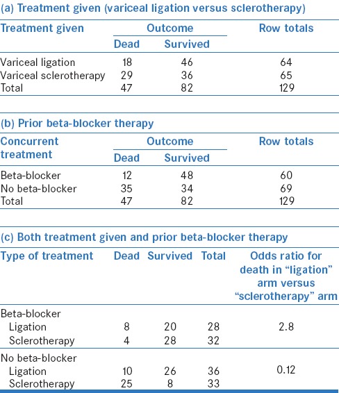
Let us consider the example of a hypothetical study to compare two treatments, variceal ligation and sclerotherapy, in patients with esophageal varices [Table 1a]. A simple (univariate) analysis reveals odds ratio (OR) for death in the sclerotherapy arm of 2.05, as compared to the ligation arm. This means that a person receiving sclerotherapy is nearly twice as likely to die than a patient receiving ligation (please note that these are odds and not actual risks – for more on this, please refer to our article on odds and risk).[2]

Table 1.

Relation of death (a dichotomous outcome) with (a) treatment given (variceal ligation versus sclerotherapy), (b) prior beta-blocker therapy, and (c) both treatment given and prior beta-blocker therapy

We, however, know that factors other than the choice of treatment may also influence the risk of death. These could include age, gender, concurrent beta-blocker therapy, and presence of other illnesses, among others. Let us look at the effect of beta-blocker therapy on death by constructing a 2 × 2 table [Table 1b]; this reveals an OR for death in the “no beta-blocker” arm of 4.1 as compared to the “beta-blocker” arm. Similarly, we can determine the association of death with other predictors, such as gender, age, and presence of other illnesses. Each of these analyses assesses the association of the dichotomous outcome variable - death - with one predictor factor; these are known as univariate analyses and give us unadjusted ORs.

However, often, we are interested in finding out whether there is any confounding between various predictors, for example, did equal proportion of patients in ligation and sclerotherapy arms receive beta-blockers? This can be done by stratifying the data and making separate tables for two levels of the likely confounder, for example, beta-blocker and no beta-blocker [Table 1c]. From this analysis, it is obvious that ligation increased the risk of death among those receiving beta-blockers but reduced this risk among those not receiving beta-blockers. Therefore, it would be inappropriate for us to look at the effect of ligation versus sclerotherapy without accounting for beta-blocker administration. Similarly, we may wish to know whether the age of patients, a continuous variable, was different in the two treatment arms and whether this difference could have influenced the association between treatment and mortality. In fact, in real life, we are interested in assessing the concurrent effect of several predictor factors (both continuous and categorical) on a single dichotomous outcome. This is done using “multivariable logistic regression” – a technique that allows us to study the simultaneous effect of multiple factors on a dichotomous outcome.

HOW DOES MULTIPLE LOGISTIC REGRESSION WORK?

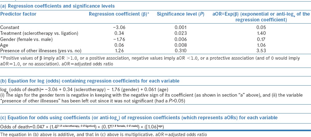
The statistical program first calculates the baseline odds of having the outcome versus not having the outcome without using any predictor. This gives us the constant (also known as the intercept). Then, the chosen independent (input/predictor) variables are entered into the model, and a regression coefficient (known also as “beta”) and “P” value for each of these are calculated. Thus, the software returns the results in a form somewhat like [Table 2a]. The “P” value indicates whether the particular variable contributes significantly to the occurrence of the outcome or not. These results can also be expressed as an equation [Table 2b], which includes the constant term and the regression coefficient for each variable, which has been found to be significant (usually using P < 0.05). The equation provides a model which can be used to predict the probability of an event happening for a particular individual, given his/her profile of predictor factors.

Table 2.

Different methods of representing results of a multivariate logistic analysis: (a) As a table showing regression coefficients and significance levels, (b) as an equation for log (odds) containing regression coefficients for each variable, and (c) as an equation for odds using coefficients (or anti-loge) of regression coefficients (which represents adjusted odds ratios) for each variable

The coefficients represent the logarithmic form (using the natural base represented by “e”) of odds associated with each factor and are somewhat difficult to interpret by themselves. The software tools often also automatically calculate antilogs (exponentials; as shown in the last column of Table 2a) of the coefficients; these provide adjusted ORs (aOR) for having the outcome of interest, given that a particular exposure is present, while adjusting for the effect of other predictor factors. These aORs can be used to provide an alternative representation of the model [Table 2c].

For categorical predictors, the aOR is with respect to a reference category (exposure absent). For example, the aOR for treatment gives the chance of death in the sclerotherapy group as compared to the ligation group, i.e., patients receiving sclerotherapy are 1.4 times likely to die than those receiving ligation, after adjusting for age, gender, and presence of other illnesses. For gender, it refers to the odds of death in women versus men (i.e., women are 0.25 times [one-fourth] as likely to die as males, after adjusting for type of treatment, age, and presence of other illnesses). Most software tools allow the user to choose the reference category. For example, for gender, one could choose “female” as the reference category – in that case, the result would provide the odds of death in men as compared to women. The results would obviously be different in that case – with software returning the aOR for gender of 4 (= 1/0.25), i.e., men are four times more likely to die than women after adjusting for other factors. If a factor has more than two categories (e.g., nonsmoker, ex-smoker, current smoker), then separate ORs are calculated for each of the other categories relative to a particular reference category (ex-smoker vs. nonsmoker; current smoker vs. nonsmoker).

For continuous predictors (e.g., age), the aOR represents the increase in odds of the outcome of interest with every one unit increase in the input variable. In the example above, increase in age by each one year increases the odds of death by 6% (OR of 1.06). This increase is multiplicative; for instance, an increase of age by 3 years would lead to an increase in odds of death by 1.06 × 1.06 × 1.06 (or [1.06]³).

As discussed in our previous article on odds and risk,[2] standard errors and hence confidence intervals can be calculated for each of these aORs. Many software programs do this automatically and include these values in the results table. Further, these softwares also provide an estimate of the goodness-of-fit for the regression model (i.e., how well the model predicts the outcome) and how much of the variability in the outcome can be explained by each predictor.

STATISTICAL TECHNIQUES FOR REGRESSION MODELS

Various methods have been proposed for entering variables into a multivariate logistic regression model. In the “Enter” method (which is the default option on many statistical programs), all the input variables are entered simultaneously. Alternative methods include “forward stepwise” regression (where various factors are introduced one by one, beginning with the strongest, and stopping when addition of the next factor does not significantly improve prediction), “backward stepwise” (where all the factors are initially introduced and then various factors are withdrawn one by one, till the overall prediction does not deteriorate), or bidirectional (a mix of the forward and backward methods).

CAUTIONS AND PITFALLS

Choosing the right predictor variables

The key to a successful logistic regression model is to choose the correct variables to enter into the model. While it is tempting to include as many input variables as possible, this can dilute true associations and lead to large standard errors with wide and imprecise confidence intervals, or, conversely, identify spurious associations. The conventional technique is to first run the univariate analyses (i.e., relation of the outcome with each predictor, one at a time) and then use only those variables which meet a preset cutoff for significance to run a multivariable model. This cutoff is often more liberal than the conventional cutoff for significance (e.g., P < 0.10, instead of the usual P < 0.05) since its purpose is to identify potential predictor variables rather than to test a hypothesis. In addition, one needs to consider the scientific plausibility and the clinical meaningfulness of the association. For instance, univariate analyses for risk factors for myocardial infarction may show that gray hair and baldness are associated with the occurrence of disease. However, these associations are scientifically implausible (and are due to association of these findings with older age and male sex, respectively) and hence must not be entered into a logistic regression analysis.

Avoiding the use of highly correlated variables

If input variables are highly correlated with one another (known as multicollinearity), then the effect of each on the regression model becomes less precise. Let us consider a model where both height and body surface area have been used as input variables to predict the risk of developing hypertension. Because body surface area depends on and therefore, has a high correlation with height, the effect of height on hypertension will get split between the two variables (and hence diluted). In such cases, the regression model should include only one of the two or more inter-related predictors.

Restricting the number of variables entered into a multivariate logistic regression model?

It has been suggested that the data should contain at least ten events for each variable entered into a logistic regression model.[3] Hence, if we wish to find predictors of mortality using a sample in which there have been sixty deaths, we can study no more than 6 (=60/10) predictor variables. However, the validity of this thumb rule has been questioned.[4]

Odds versus risk

It must be remembered that logistic regression provides aORs for each predictor. The odds differ from the risk, and while the odds may appear to be high, the absolute risk may be low.[2]

Handling continuous input variables

For continuous data (e.g., age, height, or weight), it is tempting to divide the subjects into categories (e.g., age >50 years vs. age ≤50 years). This is not a good practice since the cutoffs tend to be arbitrary and part of the information is lost.

Assumptions regarding the relationship between input and output variables

Regression models assume that the relationship between the predictor variables and the dependent variable is uniform, i.e., follows a particular direction – this may be positive or negative, linear or nonlinear but is constant over the entire range of values. This assumption may not hold true for certain associations – for example, mortality from pneumonia may be higher at both extremes of age. Therefore, calculating aORs for age as a predictor of mortality from pneumonia will not give valid results if the ages extended from neonates to the elderly. Furthermore, regression equations derived from a specific set of patients (e.g., in a developed country with advanced medical care) may not apply to patients with different characteristics (e.g., in areas without intensive care units).

SUGGESTED READING

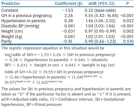
Antwi et al. developed and validated a prediction model for gestational hypertension (GH).[5] They first compared groups of women with and without GH, using the independent t-test for continuous variables and the Chi-square test for categorical variables (univariate analyses). Predictors that were found to be related to GH (P ≤ 0.20) were then entered into a multivariable logistic regression model, using stepwise backward selection. The final model with aORs for the various predictors is shown in Table 3. Readers may like to read this paper as a practical example.

Table 3.

Results of a multivariate logistic regression model to predict gestational hypertension (GH)

Financial support and sponsorship

Nil.

Conflicts of interest

There are no conflicts of interest.

REFERENCES

- 1.Aggarwal R, Ranganathan P. Common pitfalls in statistical analysis: Linear regression analysis. Perspect Clin Res. 2017;8:100–2. doi: 10.4103/2229-3485.203040. [DOI] [PMC free article] [PubMed] [Google Scholar]
- 2.Ranganathan P, Aggarwal R, Pramesh CS. Common pitfalls in statistical analysis: Odds versus risk. Perspect Clin Res. 2015;6:222–4. doi: 10.4103/2229-3485.167092. [DOI] [PMC free article] [PubMed] [Google Scholar]
- 3.Peduzzi P, Concato J, Kemper E, Holford TR, Feinstein AR. A simulation study of the number of events per variable in logistic regression analysis. J Clin Epidemiol. 1996;49:1373–9. doi: 10.1016/s0895-4356(96)00236-3. [DOI] [PubMed] [Google Scholar]
- 4.Vittinghoff E, McCulloch CE. Relaxing the rule of ten events per variable in logistic and Cox regression. Am J Epidemiol. 2007;165:710–8. doi: 10.1093/aje/kwk052. [DOI] [PubMed] [Google Scholar]
- 5.Antwi E, Groenwold RH, Browne JL, Franx A, Agyepong IA, Koram KA, et al. Development and validation of a prediction model for gestational hypertension in a Ghanaian cohort. BMJ Open. 2017;7:e012670. doi: 10.1136/bmjopen-2016-012670. [DOI] [PMC free article] [PubMed] [Google Scholar]