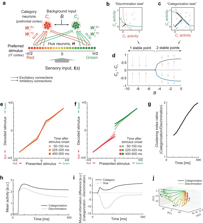
Figure 6. Bifurcation of attractor dynamics in a simple neural circuit model.
(a) Schematic of the model circuit architecture. IT hue-selective neurons (hereafter, hue-neurons), , with different preferred stimuli (varying from red to green) receive sensory input, , from the earlier visual cortex. The hue neurons interact with category neuron groups and through bottom-up and top-down connections with weights (, ) and (, ), respectively. The category neurons also receive a common background input, , whose magnitude depends on task context. Note that the modeled hue-neurons covered entire hue circle, [-π, π], although the figure shows only the half of them, corresponding to the stimulus range from red to green. (b) Activity evolution represented in the space of category-neurons in the discrimination task (where the background input ). The red (dashed) and green (solid) curves represent nullclines for category-neurons 1 and 2, respectively. The black line shows a dynamical trajectory, starting from (0, 0) and ending at a filled circle. The gray arrows schematically illustrate the vector field. (c) The same analysis as in panel c but in the categorization task (where ). The black and blue lines show two different dynamical trajectories, starting from (−0.01, 0.01) and (−0.01, 0.01), respectively (indicated as numbers ‘1’ and ‘2’ in the figure), and separately ending at filled circles. (d) The number of stable fixed points is controlled by the parameter B. Here, the parameter B was continuously varied as the bifurcation parameter while the other parameters were kept constant. The vertical axis shows the difference of category neuron activities, , corresponding to the fixed points. The solid black and blue curves show the stable fixed points; the dashed line indicates the unstable fixed point. The stimulus value was s = 0. (e–k) The model replicates recorded neural population dynamics. (e) Presented and decoded stimuli. The same analysis as in Figure 2b was applied to the dynamics of the modeled hue-neurons. (f) The same as panel e, except that the trials were segregated based on the choices (i.e., to which fixed point the neural states were attracted). The plot corresponds to Figure 3d. (g) Evolution of difference in the decoded color, corresponding to Figure 3e. (h) Mean activity of the entire neural population, corresponding to Figure 2c, inset. (i) Differences in mutual information about category and hue between the categorization and discrimination tasks, corresponding to Figure 4c. (j) The activity trajectories of the modeled hue-neurons population in PCA space, corresponding to Figure 5a. Note that the scaling of the stimulus coordinate (ranging from to ) used in the model is not necessarily identical to that of experimental stimuli (index by colors #1 – #11), and point of this modeling is to replicate the qualitative aspects of the data.


