

Abstract
A variety of medical image segmentation problems present significant technical challenges, including heterogeneous pixel intensities, noisy/ill-defined boundaries and irregular shapes with high variability. The strategy of estimating optimal segmentations within a statistical framework that combines image data with priors on anatomical structures promises to address some of these technical challenges. However, methods that rely on local optimization techniques and/or local shape penalties (e.g., smoothness) have been proven to be inadequate for many difficult segmentation problems. These challenging segmentation problems can benefit from the inclusion of global shape priors within a maximum-a-posteriori estimation framework, which biases solutions toward an object class of interest. In this paper, we propose a maximum-a-posteriori formulation that relies on a generative image model by incorporating both local and global shape priors. The proposed method relies on graph cuts as well as a new shape parameters estimation that provides a global updates-based optimization strategy. We demonstrate our approach on synthetic datasets as well as on the left atrial wall segmentation from late-gadolinium enhancement MRI, which has been shown to be effective for identifying myocardial fibrosis in the diagnosis of atrial fibrillation. Experimental results prove the effectiveness of the proposed approach in terms of the average surface distance between extracted surfaces and the corresponding ground-truth, as well as the clinical efficacy of the method in the identification of fibrosis and scars in the atrial wall.
Keywords: Bayesian Segmentation, Parametric Shape Priors, Atrial Fibrillation, Graph-Cuts, Mesh Generation, Geometric Graph
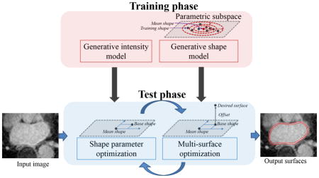
Graphical Abstract
1. Introduction
Medical image segmentation typically deals with partitioning an image into multiple regions representing anatomical objects of interest. A three-dimensional segmentation can be viewed as either a pixel classification (defining regions) or a surface estimation (boundaries of regions), and in this paper we deal with the latter approach. Heterogeneous pixel intensities, noisy diffuse boundaries and irregular shapes are some factors that make it difficult to develop accurate, robust segmentation algorithms for certain classes of images and anatomy. The proposed method is motivated by a particular problem of this type, which is the segmentation of the left atrium (LA) wall, also referred as the myocardium, from the late-gadolinium enhancement cardiac MRI (LGE-MRI) in patients suffering from atrial fibrillation (AFib) (Benjamin et al., 1994; Go et al., 2001).
Considering the case of the left atrium, the manual segmentation of the LA wall entails the delineation of its inner and outer surfaces, namely the endocardium and epicardium. These manual segmentations can be time-consuming (approximately one hour per image) and require significant manpower with sufficient domain-specific expertise. Furthermore, these segmentations are prone to inconsistencies among experts. Automatic segmentation, on the other hand, promises to be an economical solution to such problems, with the benefit of reducing human variability or bias. Figure 1 shows samples of such images where one can appreciate the challenges of extracting a thin wall structure (2–5 mm (Ho et al., 2012)) with weak boundaries and complex geometry. Further, these structures suffer from contrast variation, low signal-to-noise ratio and motion artifacts (Peters et al., 2007).
Figure 1.

LA wall challenges: Slices of LGE-MRI images showing the challenges in segmentation. The left two 2D slices are shown without manual delineations of the LA wall, and the right two slices show manual delineations.
To address the challenges of difficult segmentation problems like the LA wall, we propose a surface estimation scheme with the following aspects. First, it should handle various degrees of noise and estimate surfaces with ill-defined boundaries. Second, it needs to simultaneously estimate multiple surfaces in a globally optimal manner. Next, it should preserve the topology of the desired surface by taking into account the shape population of interest. Finally, the reconstructed surfaces are required to be regularized to compensate for misleading intensity information.
Current segmentation approaches handle such problems, but they are lacking in one way or another. For example, weak boundary segmentation problems are often solvable only by inducing an a priori notion of the shape characteristics in question. This triggers a strong motivation for a Bayesian framework for segmentation, which includes statistical models such as active shape models (ASM) (Cootes et al., 1995) and many variations derived from that approach. However, these models restrict the solution to lie only in a low-dimensional shape space defined through the training data. In cases like LA, clinicians require the output surfaces to follow correct boundaries rather closely and yet coarsely similar to a significant summary of the training dataset. Lower-level deformable shape methods, such as level sets (Malladi et al., 1995; Whitaker, 1994), which typically rely on gradient descent optimizations, have been shown to be unable to handle such large variations in the boundary contrast. Moreover, statistical and deformable methods rely on some sort of incremental fitting algorithm that is prone to get trapped in local minima during optimization, which has been demonstrated in (Veni et al., 2013). The difficulty in optimizing shape models in the presence of such a challenging environment motivates us to consider an optimization strategy that seeks a globally optimal solution. In particular, graph-cuts provide a flexible global optimization tool with significant computational efficiency. Boykov and Kolmogorov (Boykov and Jolly, 2001; Kolmogorov and Zabih, 2004) developed efficient algorithms by using graph-cuts to segment regions optimally in the n-D image data. However, these methods are region-based and are not necessarily meant to extract features specific to the desired surface as verified by (Veni et al., 2015). Moreover, they do not preserve the topology of the desired surface and use approximations while dealing with multiregion segmentation (Boykov et al., 2001). To extract multiple interlinked surfaces, (Sonka et al., 2007) used an optimal surface net approach. However, the technique embeds hard geometric constraints on surfaces smoothness and their interrelations, which lead to irregular output surfaces.
In this paper, we address these issues by developing a surface-based segmentation algorithm with several important features that address unmet technical challenges in a range of applications. The primary features of our formulation include: (1) the reliance on a generative model that incorporates a global shape prior, (2) controlled smooth deviations from that prior that lead to soft penalties and eventually result in regular output surfaces, (3) a learned model of intensity patterns, (4) a combination of a shape-based linear system and the graph-cut approach (and hence we refer to this framework as ShapeCut) to globally maximize the parametric shape prior and the surface estimate in an iterative fashion and (5) simultaneous extraction of multiple surfaces.
Thus, the resulting surface-based image segmentation algorithm develops a generative image model by incorporating both global and local shape priors in the energy minimization framework. Unlike previous shape models (Cootes et al., 1995, 2001a) that impose over-restrictive shape constraints by limiting the solution to some learned subspace of shapes, the proposed algorithm allows deviations from this subspace, in a rather controlled fashion, by means of local shape priors. These deviations accommodate test data complexities that become advantageous when dealing with a limited number of data samples, a typical scenario in medical imaging applications due to much-needed labor-intensive manual segmentations. Further, the global updates-based optimization strategy that iteratively maximizes the parametric shape prior and the surface estimate makes the algorithm converge in relatively few iterations as compared to gradient-descent optimizations. This global property is also crucial when dealing with difficult segmentation problems where the desired object possesses spatially varying intensity patterns due to surrounding tissues that possess similar image properties. While learning the spatially varying intensity patterns, the generative intensity model is formulated by incorporating the covariance structure that typically exists among intensity patterns in the training set, unlike the approach described in (Veni et al., 2015).
The remainder of the paper is organized as follows. In Section 2, we provide the necessary background related to the presented work. In Section 3, we provide the theory behind ShapeCut, which includes shape-based generative modeling and the two fast global optimization strategies. Section 4 presents experimental results followed by their analysis in Section 5. Finally, we conclude with a summary of our approach in Section 5.4 along with future directions.
2. Related Work
The relevant work falls into several different categories based on the approach and the effectiveness/efficiency for tasks relevant to the goals of this paper. We begin with the image segmentation methods based on shape priors that are learned from a set of training examples. This category includes active shape models (ASM) (Cootes et al., 1995) and active appearance models (AAM) (Cootes et al., 2001a), which rely on training data with correspondences/ landmarks and assume a Gaussian density in the low-dimensional subspace of landmark-based shape representations. Variations include nonparametric shape priors in the subspace defined by principle component analysis (PCA) of signed distance transforms (Kim et al., 2007). Extending these methods that learn a low-dimensional shape prior, the proposed work relies on a low-dimensional subspace derived from the training shapes, but also accommodates perturbations from this relatively confined space. Furthermore, the proposed method relies on minimization schemes that optimize segmentations and shape parameters in a global fashion, rather than relying on incremental, gradient descent-based schemes.
The second class of segmentation methods falls under the category of pixel-labeling-based energy minimization schemes. Boykov and Kolmogorov (Boykov and Jolly, 2001; Kolmogorov and Zabih, 2004) used this scheme to segment objects in N-dimensional images. Energies typically include a regional term that quantifies the incompatibility of each pixel with a given region (e.g., foreground, background), and a smoothness term that defines the extent to which a region/labeling is piecewise smooth. To optimize such energy, graph-cuts have been shown to be efficient and globally optimal. However, these methods are best when they rely either on an initial set of seed points or on region-based penalties (Li et al., 2006). Further, they do not readily incorporate shape-based information. The resulting segmentation tends to be biased toward regions similar to the seed points and may not preserve the topology of the underlying surface. Thus, pixel-labeling methods cannot be applicable for the LA wall segmentation due to the localized intensity patterns surrounding the left atrial region and its shape complexity.
Malcolm et al. (2007) extended the pixel-labeling graph-cuts framework by incorporating nonlinear shape priors. They used kernel PCA from a set of training shapes followed by iterative graph-cuts to segment the desired object, thus loosing the global nature of the original graph-cuts optimization. Xiang et al. (2013) proposed a pose-invariant pixel-labeling segmentation approach by incorporating a discrete shape model via a set of higher order cliques. They solved the derived energy simultaneously in both model and image space by using a tree-reweighted-sequential (TRW-S) message-passing optimization algorithm, which is not guaranteed to produce a global minimum (Saito et al., 2016). Vu and Manjunath (2008) used a discrete version of the signed distance function to represent the shape prior within the level-set framework. Then, they merged this shape prior with the regional term of the minimizing energy and optimized it using graph-cuts. Recently, Gorelick et al. (2013) proposed a trust region approach to optimize the pixel-labeling-based segmentation energy that includes the nonlinear region terms, surface area penalties and shape priors based on image moments. Within the trust region, they solved the nonlinear approximation of the underlying energy via graph-cuts. On the other hand, we view the segmentation problem as a surface estimation problem, rather than a pixel-labeling problem, that accommodates shape complexity and localized intensity patterns surrounding the surface being extracted. Thus, we introduce the shape priors in a more systematic, Bayesian framework and learned surface features (rather than region penalties), which are particularly important for the class of problems studied in this paper. In addition, the proposed framework simultaneously extracts multiple interlinked surfaces in a globally optimum manner. Although Delong and Boykov (2009) and Schmidt and Boykov (2012) proposed a pixel-labeling-based segmentation framework that extracts multiple regions by using a single graph-cut, it is very difficult to encode parameterized shape priors in their graph structure. Further, their framework lacks enforcing of smoothness constraints over the individual surfaces, which results in producing irregular boundaries. This has been shown in Section 4.4.
In order to deal with surface based features, deformable-surface methods such as level sets (Whitaker, 1994; Malladi et al., 1995) can be used along with shape priors to extract the desired surfaces. For example, (Rousson and Paragios, 2002), (Chan and Zhu, 2005) and (Cremers et al., 2006) used shape priors in their level sets-based segmentation framework. However, like statistical shape models, deformable surface methods use gradient descent-based optimization approaches that are sensitive to initializations and are prone to get trapped in local minima.
The work most relevant to the proposed method is based on the optimal net surface problems on a special geometric graph structure introduced by Wu and Chen (2002) and its applications to medical image segmentation (Li et al., 2004; Song et al., 2013). Wu and Chen designed a graph in the form of a multicolumn properly ordered (PO) graph, and they proved the equivalence between the image segmentation problem and min-cut on the s−t graph via optimal net surface problems, thus providing a globally optimal and efficient solution. These surface-net problems induce costs on surfaces rather than on regions and do not rely on approximate (suboptimal) solutions when applied on multiple surfaces (Li et al., 2005), motivating its practical use in surface-based segmentation approaches. Li et al. (2005, 2006); Dou et al. (2008); Song et al. (2009); Li et al. (2011) used one of the surface-net approaches in the form of a V-weight net surface problem to simultaneously extract multiple interrelated surfaces in multiple clinical applications. Song et al. (2013) extended this idea by introducing shape priors into such surface estimation schemes, but the priors were strictly local, implemented as modifications to smoothness parameters in the optimal cut formulation. Veni et al. (2013) used an another form of the surface-net approach, namely, a VCE-weight net surface problem by enforcing soft constraints on surface smoothness and interrelations between coupled surfaces. However, they do not incorporate parameterized shape priors in their Bayesian formulation, which is essential for the LA wall segmentation.
The proposed work introduces a parameterized shape space and estimates global shape parameters in a closed form for segmentation as a part of the optimization process. Furthermore, the integration of shape space keeps it separate from the mesh/graph. Thus, the graph becomes, essentially, a discrete approximation to an underlying continuous parameterization of a subset of the 3D volume. The work in this paper builds on the previous work of the authors (Veni et al., 2013, 2015). The paper also discusses further improvements in the generative intensity model by embedding the covariance structure that exists between intensity profiles. We also talk about the gradient vector flow (GVF)-based nested mesh building strategy, which, in turn, defines the multicolumn graph. Further, the paper provides an extensive formulation of the shape prior model on coupled surfaces. With respect to the evaluation of results, we performed a thorough analysis of every aspect of the underlying model. Apart from the qualitative and quantitative analysis of segmentation results, we carried out their clinical evaluation, which could elucidate the effectiveness of the proposed work even from a clinical viewpoint.
3. Methodology
We treat the image segmentation as an energy minimization problem over the surface 𝒮 to be estimated. Within a Bayesian framework, this energy minimization can be cast as a maximum-a-posteriori (MAP) estimation, where the log-posterior of the desired surface is maximized for a given image. However, the proposed work differs from many other Bayesian methods in that the underlying search space is an approximation of a continuous parameterization of the set of possible surfaces, as shown in Figure 2a. We discretize the underlying continuous parameterization in the form of a special form of geometric graph structure, in order to simultaneously estimate multiple, interacting surfaces in a globally optimal manner. Figure 2b depicts the strategy representing the continuous parameterization in the form of a discrete graph whose design involves a set of nested layers and columns. Here, each layer maintains a similar topological structure to that of the desired surface, and each column necessarily ensures the estimated surface to pass through it. For the 2D surface estimation, these layers represent 2D discrete contours, and in the case of 3D, these layers become meshes.
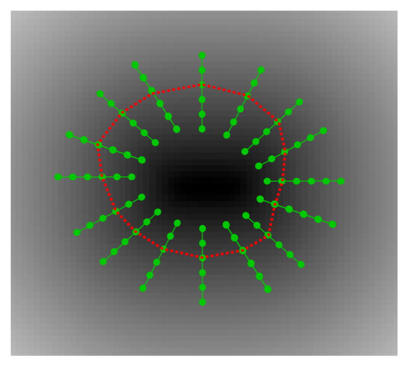
Figure 2.

Parametric search space: Schematic showing a (a) continuous parameterization of the surface estimate 𝒮, (b) discrete approximation of the underlying continuous parameterization within which the surface estimation takes place and (c) overlay of discrete grid on a given image and intensity profiles, pi,j (yellow) at different grid points xi,j.
We begin by defining the graph structure along with the associated notations. The graph 𝒢 = (𝒱, ℰ) is represented by a set of columns and a neighborhood structure among adjacent columns, and hence is referred to as a multicolumn graph. This multicolumn graph is formed by a set of vertices 𝒱 and a set of edges ℰ that are connected in a properly ordered fashion (Wu and Chen, 2002). The graph has I columns and J vertices along each column, forming J layers. Each column has a set of 3D vertices along its length. Thus, the columns span the 3D space in which the segmentation takes place. A particular vertex at the jth position along ith column is associated with a 3D location xi,j in a given volume. Thus, a surface 𝒮 is the set of nodes 𝒮 = {s(i) ∈[1, J]}, ∀i ∈[1, I] representing the position of the surface along each column. Associated with each vertex is an intensity profile that may consist of either a 3D patch or a 1D array of intensities pi,j (e.g., oriented along the approximate normal to the surface), as shown in Figure 2c. Thus, a particular surface (set of vertices) induces a probability on a set of image intensities around each point on the surface.
3.1. Bayesian Formulation
Here we introduce the Bayesian model to express the posterior probability of a surface 𝒮 as a function of the given image I. Using Bayes rule, we have:
| (1) |
The image likelihood, P(I|𝒮), is a generative model of intensities in the vicinity of a particular surface estimate. Veni et al. (2013) defined the image intensity model by means of a set of training images with an isotropic Gaussian distribution around a learned mean. Here we model the intensity profiles for a surface at a column location with a column-dependent mean, μi and covariance Σi. Following (Veni et al., 2013), the generative models for intensities are computed by analyzing the intensity profiles that lie within a predefined radius r of points on the column. We model the intensity profiles at different points on the surface as independent, and therefore the log of the conditional probability is:
| (2) |
The surface prior, P(𝒮), is a generative model for surfaces. For this work, we use a linear model and an associated set of latent variables, β, to represent global shape information. This linear model is learned over training shapes, and captures low-dimensional properties of shape representation, as in (Cootes et al., 1995). To account for the actual complexity of the left atrium, the generative shape model allows smooth deviations or offsets from the low-dimensional shape distribution, formulated as a Markov random field (MRF) prior on their configuration. As a result, the proposed surface prior, P(𝒮), captures global and local characteristics of the desired surface. Ideally, because β is a latent variable, we formulate the complete prior in terms of a marginalization over β:
| (3) |
Computing P(𝒮) as an integral over all instances of β is generally intractable. However, in the case of Gaussian distributions, we can assume that the integral in (3) is sharply peaked at a most probable latent setting βMP where classical dimensionality reduction techniques provide a closed-form solution. Hence, we approximate the integral of (3) using a point estimate of β, and thus we have:
| (4) |
where the point estimate βMP can be interpreted as the mean of latent posterior, p(β|𝒮), as in (Tipping and Bishop, 1999). This approach becomes the conventional maximize-maximize (max-max) formulation of parameter estimation in the context of latent variable models. The max-max algorithm is a special case of the expectation-maximization (EM) algorithm that relies on the point estimate of latent variables of a model rather than a distribution. In other words, EM deals with the expectation of latent variables (in this case, shape parameters), which involves integration to estimate the posterior distribution, whereas the max-max algorithm mitigates the challenge of this integration in order to get the point estimate by assuming that the posterior is sharply peaked around its mode. Hereafter, we will refer to the latent point estimate as β for notational convenience.
Figures 3a and 3b show a simplified geometric interpretation of the model. The linear subspace, which is learned from training data, is relatively low-dimensional, but allows the segmentation algorithm to operate effectively when parts of the anatomy are not well delineated in the image data, typically because of low-contrast and high-correlated and/or uncorrelated noise. A shape is generated from a position β on this low-dimensional shape representation (shown as a 2D space in Figure 3), and we refer to β as shape parameters.
Figure 3.

Shape representation within and off the subspace: Schematic showing (a) training shapes implicitly represented by distance transforms, (b) projection of shapes onto a linear subspace and (c) estimated surface 𝒮 derived from the deviation, 𝒮o, of the base shape 𝒮β.
To represent and learn this shape space, we use the signed distance transform (DT) of the training data. Thus, for each training segmentation, namely d, whose zero level set corresponds to the surface boundary, we use principal component analysis (PCA) on the set of training DTs and choose a low-dimensional linear subspace that maintains 95% of the shape variability to model shape parameters (Leventon et al., 2000). From the training data, we also estimate a Gaussian distribution over the shape parameters, and therefore:
| (5) |
where ΛK is the diagonal matrix of K largest eigenvalues derived from the PCA. The eigenvectors (eigen DT) dek from PCA, along with a specific set of shape parameters β, give rise to a particular DT, which we denote dβ:
| (6) |
where x ∈ℜ3 is the particular image location and dμ denotes the mean DT. The zero level set of the base distance transform, 𝒮β = {x|dβ(x) = 0} plays an important role in expressing the conditional surface probabilities, in terms of both a base shape and an offset.
Unlike previous shape-prior-based image segmentation methods, which restrict the surface estimate to remain in the low-dimensional subspace, the proposed method also allows offsets from this subspace while introducing a covariance structure on these offsets. To allow the offset, we model the conditional surface probability, P(𝒮|β), in the form of MRFs. The MRF model enforces correlation among nearby points on the surface while prioritizing smooth deviations from the linear model learned from a set of training shapes. We let 𝒮o be defined as an offset from the base shape, 𝒮β, which lies in the subspace. Thus, the surface estimate 𝒮 is given by 𝒮β + 𝒮o (as in Figure 3c). For a given set of shape parameters β, the surface probability depends only on the offset (𝒮 ≡ 𝒮o), which we penalize so that it should be small (the shape should be similar to the base shape) and smooth (nearby columns should have similar offsets). Therefore, the negative log conditional probability of the surface for a given β can be defined as:
| (7) |
where σo and σ𝒞 are standard deviations of surface offsets learned from the training set and the neighborhood structure, defined by 𝒞, which is the clique in the base graph defined over the base shape. According to the MRF, the first term of (7) defines the unary potential of the negative log-likelihood of the surface, 𝒮, given shape parameters, β, so that it encodes relatively small offsets from the linear subspace. The second term defines the pairwise clique potential, which encodes smooth deviation of 𝒮 from the linear subspace. The combined effect of the unary and pairwise clique potentials allows the surface estimate to deviate from a low-dimensional linear subspace.
To express P(𝒮|β) in (7) on the proposed grid, we use the following approximation. For a given β, we build the base shape 𝒮β by computing the intersection of each column i with the zero crossing of dβ, to give a vertex and 3D positions for sβ(i). The magnitude of the offset 𝒮o from 𝒮β is the distance along each column relative to the base shape, and the contribution to the log-prior is therefore , where si = xi,s(i), the sum of square distances of the vertices along each column i from the base shape.
Combining (2), (5) and (7), we derive the negative log-posterior of a surface 𝒮, given an input image I:
| (8) |
The above derivation results in a shape-based generative model of an image that describes the intensity patterns associated with the shape of the left atrium. A point β in the low-dimensional PCA subspace, chosen from a multivariate normal distribution, gives rise to a distance transform, whose zero level set is the base shape, 𝒮β. An offset from 𝒮β is chosen from an MRF distribution, which extends the learned probability distribution from the PCA subspace into the entire shape space in a way that favors smooth shapes that are very near to but do not exactly resemble the training set. Finally, each point on that surface gives rise to an array (patch or vector) of image intensities that are drawn from a (identically, independently) Gaussian distribution, with a mean and covariance that are learned from the training data along each column.
3.2. Extension of Bayesian Formulation to Multiple Surfaces
The LA wall segmentation problem consists of a pair of nested surfaces— the epicardium and endocardium—which we denote 𝒮1 and 𝒮2, respectively. We extend the above formulation so that the distance transforms are modeled jointly. Similar to (Veni et al., 2013), we introduce a penalty on the intersurface distances (expressed in the same probabilistic framework, learned from the data, and tied to the β-shape-pair, that is β1 and β2) such that the surfaces are estimated optimally in a joint formulation. Therefore, the combination of (1) and (4) can be modified for two surfaces as follows:
| (9) |
For this work, we assume that the intensity models for each column corresponding to epi- and endocardial surfaces are independent of each other with different mean intensity profiles and and covariance structures and , respectively. Likewise, we apply the independence assumption over shape parameters β1 and β2. Following this, the probabilities for intensity and shape models are applied in a similar way for both surfaces as expressed in (2) and (5). Since β2 is implicitly related to 𝒮2 while simplifying for P(𝒮1|𝒮2, β1, β2) and β1 remains fixed for P(𝒮2|β2, β1), (9) can be further simplified as:
| (10) |
To express the conditional surface probabilities, P(𝒮1|𝒮2, β1) and P(𝒮2|β2), we account for the mutual relationship among the coupled surfaces apart from the individual surface estimates. By modeling 𝒮1 with a normal distribution on distance to 𝒮2, the negative log of the joint surface estimate is:
| (11) |
where Δ(i) denotes the ideal intersurface distance for column i, which is learned by averaging the differences between the intersection of that column with the zero level sets of two interlinked signed distance transforms (in our case, epi-and endocardium) over the training set. The intersection of the multicolumn graph with the zero level set of a signed distance transform has been illustrated in Figure 4. σ𝒞′ represents the standard deviation of this distance, which can also be learned from the training data. For simplicity, let the intersurface relationship between the epi- and endocardial surfaces, s1(i) − (s2(i) + Δ(i)), be denoted by ρ. Because the epicardial surface is always above the endocardial surface, we let ρ < −Δ(i). This condition ensures that s1(i) < s2(i) for any given mesh column and eventually avoids either crossing or overlapping of coupled surfaces. Therefore, the negative log-posterior of coupled surfaces 𝒮1 and 𝒮2, and shape parameters, β, with an input image I, is given by:
| (12) |
Figure 4.
Multicolumn graph-zero level set intersection: Schematic showing the intersection (red curve) of the multicolumn graph with the zero level set of a signed distance transform corresponding to a surface from the training set. Likewise, this intersection is sought for all the training examples. This process is repeated for the other surface. The average of the differences between the intersections of two surfaces gives the Δ.
3.3. 3D Mesh Construction
The proposed Bayesian formulation over 𝒮 on a surface-conforming multi-column graph structure requires a 3D nested mesh that defines a 3D subdomain that contains the surfaces to be estimated. We propose a mesh building strategy that relies on a set of training samples.
As seen in Figure 5, the shapes of the left atrium are highly variable, especially within and around the veins that come out of it. This variability is captured by the statistical model, described above, and the use of training data for the estimation of the computational domain.
Figure 5.

Variability of left atrium shapes.
In order to construct a 3D nested mesh structure, we initially need to build a base mesh that complies with the training set of segmented shapes. We begin by rigidly aligning the training set of segmented images, using FSL-FLIRT (Jenkinson and Smith, 2001) to perform the pairwise registration step to a group atlas. In particular, with 7 degrees of freedom (translation, rotation and scaling), we align each training shape to an iteratively evolving average (template) until convergence (i.e., a rigid with-scale unbiased atlas building strategy over all training shapes). To build our nested mesh model, we use the mean signed distance transform (DT), dμ from the aligned training shapes. The zero-level set of dμ gives rise to a filtered distance transform d̃μ with respect to the average shape, using the Fast Marching Method (FMM). Using marching cubes and subsequent decimation and resampling to improve quality (Valette et al., 2008), we have a triangulated base mesh with relatively good mesh quality (aspect ratios and triangle sizes).
Once the base mesh is generated, we construct nested mesh layers that represent a collection of offset surfaces, both inside and out. For this, we use a gradient vector flows (GVF)-based nested mesh building strategy (Bauer et al., 2011) derived from the filtered distance field, d̃μ. As long as the filtered signed distance transforms are smooth, the columns generated using the gradient vector intersect only at local extrema in the distance tranform. This places a limit on the number of the layers. Thus, the search space for the solution is limited to the local feature size of the surface (Amenta et al., 1998).
Starting at each node of the base mesh, we traverse along the direction of the gradient vectors while creating new nodes successively. These nodes are eventually used to construct graph columns. Specifically, consider a node in a mesh that is located at . To acquire a corresponding node for the next mesh layer, either inside or outside the base mesh, we apply:
| (13) |
where δ denotes the distance between two successive mesh layers and represents the zero-level set of d̃μ. A collection of all the nodes forms a new mesh layer that maintains the topology of the base mesh. This action continues so that the nested mesh layers cover the required computational domain. For our application, the number of mesh nodes per each layer corresponds to 12665 for the heart data and 6262 for the synthetic data. Based on the capture range of two surfaces, we generated 75 mesh layers, spaced at 0.5 voxels each, which occupy a capture range of 38 voxels for the final surface estimate.
3.4. Optimization
To seek a globally optimal solution for 𝒮 and β, we follow a conditional maximization scheme in which we iterate between two relatively fast, global optimization phases. In the first phase, we optimize for 𝒮 given β, and in the second phase we optimize for β given 𝒮.
For the first phase, we use graph-cuts to solve the VCE-weight net surface problem, using (Wu and Chen, 2002). Here we use the MRF formulation (Veni et al., 2013), which follows the derivation introduced in (Ishikawa, 2003). The strategy is to express the above penalties as a set of weights on vertices and edges of a multicolumn properly ordered (PO) graph, and reduce the surface estimation problem to an s-excess cut on the graph. This produces an optimal low-order polynomial time solution–and in practice runs very fast, even for large graphs. The details of the multicolumn PO graph construction follow from (Wu and Chen, 2002), and we present here how our energy minimization-based probabilities get encoded on the vertices and edges of the PO graph.
Weights/costs on the graph vertices arise from two sources. The first source of costs is derived from the intensity model, P(I|𝒮), by sampling image patches around each vertex pi,j, and computing the negative log-likelihood from the Gaussian model, (μi,Σi). For notational convenience, we denote the negative log-likelihood by WI. The second part comes from the shape model by sampling the squared distance transform dβ of the base shape 𝒮β at each vertex position (i, j) in the form of surface offset 𝒮o and is denoted by W𝒮β. These terms are weighted by a dominance factor ω, and added to induce vertex costs Wi,j :
| (14) |
Typically, for low contrast images, ω is chosen to be less than 0.5 in order to emphasize shape-based costs over the image matching-based costs.
To build the PO graph, edges are inserted between adjacent vertices along each column carrying +∞ costs. They also go in between vertices of adjacent columns to model the pairwise clique potential C(so(i1), so(i2)), associated with the offsets, rather than the absolute positions of the surface, as in (Veni et al., 2013). For the optimization to be feasible, we use C(d) = αd2, where α represents the scaling factor on the clique potential. Typically, α regulates the penalty on the smoothness of the estimated surface, and d2 = (so(i1) − so(i2))2 comes from the surface smoothness part in (7). The configuration of the edges between adjacent columns is inherently managed by the β-shape, 𝒮β. To be specific, the intersection of 𝒮β with each graph column gives a reference position, sβ. The so’s between adjacent columns, defined by the clique potential C, are adjusted relative to sβ’s positions. Figure 6 illustrates the arc configuration with respect to the intra- and intercolumn arcs. In this way, the nested mesh on which we perform graph-cuts becomes a numerical construct and does not define or heavily influence the shapes of the objects to be segmented. If a mesh is sufficiently fine grained, it serves only to restrict the topology of the surface. For a given β, the surface estimate 𝒮, computed using graph-cuts, is the global optimum of the posterior in (1).
Figure 6.
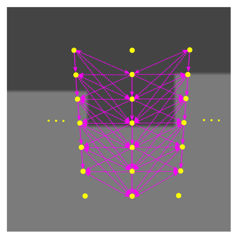
Shape complying properly ordered graph construction: Schematic showing arc configuration between adjacent columns being overlaid on a given image. The entire arc configuration assembly is deformed with respect to the base shape 𝒮β during each iteration.
In the second phase of the optimization, we compute β for a given surface 𝒮 by minimizing the negative log-posterior. This computation is done by taking the derivative of (8) with respect to β and equating it to zero. Since the negative log-posterior is quadratic in terms of β, we obtain a closed-form solution.
| (15) |
Here dβ represents the base distance transform and is expressed in (6). The images ∂dβ/∂β are the principal components. By rearranging terms in (15), the optimal shape parameters, β*, are given by:
| (16) |
| (17) |
| (18) |
In equations (17) and (18), 𝒞𝒩 represents I ×I symmetric, indicator matrix, with the corresponding elements, i ∈I, equal to 1 if i′ ∈𝒩i (neighborhood of i), else 0. Thus, (16) gives the optimal β for a given surface segmentation that finds a compromise between fitting the current segmentation and choosing a likely β based on the Gaussian distribution.
When we consider the algorithm in full, the proposed method differs significantly from others that either work strictly within the shape subspace (Cootes et al., 1995) or project intermediate solutions onto that subspace. Here, the optimization strategy offers two advantages. First, it allows intermediate results to deviate from the low-dimensional shape subspace and to pull the shape parameters, β, toward this segmented surface. Second, in each iteration we perform a global optimization of 𝒮 and β, thus relying less on local image properties near the current solution. Thus, the algorithm converges with relatively few iterations (e.g., ~5 iterations on average for results in this paper).
While dealing with the multisurface problem, we follow the same iterative conditional maximization scheme where we optimize for coupled surfaces, 𝒮1 and 𝒮2, for a given β-shape-pair in the first phase, and in the second phase, we optimize shape parameters β1 and β2 independently for 𝒮1 and 𝒮2, respectively. At each iteration, for a given 𝒮l, the mutual interaction between surfaces does not influence the estimation of shape parameters, βl, allowing each βl to be estimated independently in the same way as in (16). However, to estimate coupled surfaces for a given β-shape-pair, we consider the mutual interaction estimate and optimize the V CE-weight net surface problem using graph-cuts.
4. Results
To assess the performance of the proposed method, we applied ShapeCut on the left atrial (LA) wall segmentation from the LGE-MRI images in patients suffering from AFib. LGE-MRI imaging highlights abnormal tissue, including fibrosis, within the atrial wall (Higuchi et al., 2014). It is used for both quantifying the degree of fibrosis prior to RF ablation (a medical procedure used to treat AFib), and quantifying and tracking the effects of the RF ablation in the formation of scar tissue. As a proof-of-concept, we start by demonstrating the algorithm’s performance on 3D simulated parametric shape examples that have a coupled-surface structure similar to the LA wall.
4.1. Datasets
Synthetic dataset
We considered a class of 3D parametric shapes termed supershapes (Gielis, 2003; Fougerolle et al., 2007) whose 2D parameterization in polar coordinates can be written as:
| (19) |
The 3D extension was obtained by a spherical product:
| (20) |
where θ ∈[−π/2, π/2], ϕ ∈[−π, π] and we set a = b = 1. We generated shapes of four rotational symmetries, m = 4, to mimic pulmonary vein structures coming out of the LA. The associated shape parameters (n1, n2, n3) were drawn from χ2 distributions with four degrees of freedom. We used the implicit representation of rational supershapes in (Fougerolle et al., 2007), which yields smoother shapes compared to the standard ones in (Gielis, 2003) that suffer from sharp corners. We imitated coupled-surfaces using two level sets of r(ϕ): the zero-level set associated to the generated supershape, and a positive level set to simulate the inner surface. Using this strategy, we produced 170 volumes of size 200 × 200 × 200 where each volume contained three regions: the region inside the innermost surface (innermost region), the region in between the inner and outer surfaces (middle region) and the background. To mimic variations associated with the LA-wall thickness, we perturbed the inner and outer surfaces by introducing correlated random noise determined by convolution of random noise with a Gaussian filter of standard deviation 25 to produce smooth wiggles along both surfaces. To simulate image intensities that reflect appearance differences between distinct regions, we considered a Gaussian-distributed appearance model within each region of variance 9 and means 40, 70 and 10 for the innermost, middle and background regions, respectively. To replicate some of the MRI imaging challenges, each image was corrupted with Rician noise with variance 30 and a smoothly varying bias field.
LGE-MRI cardiac dataset
For the real-data experiments, we apply ShapeCut on the LA wall segmentation where 72 LGE-MRI volumes (37 pre- and 35 postablation, each of size 300 × 400 × 107 and isotropic resolution of 0.625 mm) were obtained retrospectively from an AFib patient image database at the University of Utah’s Comprehensive Arrhythmia Research and Management (CARMA) Center1. Along with the LGE-MRI volumes, we were provided with expert-delineated binary segmentations for the epicardium and endocardium. Of the 72 samples dataset, 62 volumes were served with a single-handed segmentations from an expert, and the remaining 10 volumes were provided with binary segmentations from three experts. These segmentations were used to generate the properly ordered (PO) graph, extract intensity features and learn the shape model and for the purpose of evaluation.
4.2. Shape Prior Construction: Training Sample Size
Learning shape priors poses convergence challenges for high-dimensional shape spaces and relatively low training sample size. Hence, it is critical to show that the underlying shape variability in a given population can be captured by a finite, probably small, number of training shape exemplars. Such training samples account for linear subspace approximation, for which even fewer eigenmodes, relative to the training sample size, would capture the population shape variability. To assess the algorithm’s performance against the number of training samples, we used a repeated random-subsampling-based resampling strategy (Politis and Romano, 1994) where repeated trials (subsets) were drawn to compute performance statistics. Figure 7 shows average scree plots from repeated random training subsets of different sample sizes for synthetic and the LA datasets. It can be observed that 95% of the shape variability can be captured by a smaller number of eigenmodes relative to the training sample size. Note that for high-dimensional shape spaces, we do not require an exact characterization of the covariance structure in the off-subspace. For a segmentation task, we allow for deviation from the shape subspace in a regularized manner in the form of MRF-based clique potentials.
Figure 7.

Eigen spectrum: Average scree plots for different training set sizes for (a) the synthetic dataset and (b) the left atrium.
Another important aspect of building shape priors is subspace consistency where the eigenmodes are reliably estimated with the given finite training set. To this end, we adopted two shape-based PCA measures, projection error and subspace error, that were computed from data subsets. These measures reflect the representation capability of the learned shape prior in terms of deriving shapes (i.e., 𝒮β) that resemble the training set while determining the deviation from the prior’s subspace (i.e., 𝒮o), which is needed to accurately represent a testing shape. Smaller errors, relative to the off-subspace noise variance, eventually help in obtaining a reliable segmentation. We define these measures as follows:
Projection error
This measure quantifies the distance between the original set of centered samples X̃ and the reconstructed samples derived from a learned shape prior. Mathematically, it is given by:
| (21) |
where, represents a set of k significant eigenvectors derived from the PCA on subsampled data for the jth trial and F represents the Frobinious norm. From the segmentation standpoint, this error provides the surface offset 𝒮o from a within-subspace shape reconstruction 𝒮β that is needed to represent a test shape. Since the surface probability demands small and smooth offsets, it is desirable to have a small projection error at the cost of the number of training samples.
Subspace error
This measure computes the distance between the reconstructed samples derived from the eigen decomposition of the subsampled data against the reconstructed samples derived from the entire data. Mathematically, it is given by:
| (22) |
where, Wk represents a set of k significant eigenvectors derived from the PCA with respect to the entire dataset. From the segmentation standpoint, it provides the distance between base shapes 𝒮β that are defined over the subspaces spanned by subsets of the dataset and the entire dataset itself. This measure encodes the consistency of prior learning using smaller training sizes as compared to the full dataset.
For both measures, we again used a repeated random-subsampling-based resampling strategy to draw multiple random samples for different sample sizes. For synthetic as well as the left atrium datasets, we chose training samples sizes ranging from 10 through 60 in the interval of 10 and drew 150 random subsets for each training size. Finally, for each subset, sample statistics were calculated from these trials. Figure 8 shows the mean and standard deviation (in noise variance units considering all training samples) of these measures by considering different numbers of subsamples. As expected, the errors decrease with the number of samples. In particular, the projection error levels off at or beyond the off-subspace noise variance for both datasets, which suggests that it served to learn shape priors with relatively small-sized training datasets (e.g., as would be available in clinical applications). Similarly, the convergence of subspace error to less than noise variance (especially for the LA data) is indicative of the shape prior robustness and consistency in learning eigenmodes that capture shape variability with a finite subset of the training shapes.
Figure 8.

Shape-based PCA measures: Projection error (top) for (a) the synthetic dataset and (b) the left atrium, subspace error (bottom) for (c) the synthetic dataset and (d) the left atrium.
4.3. Algorithm Flow
For a given test example, ShapeCut relies on user input to locate the model’s approximate center, based on which every point of the 3D nested mesh is positioned. This approach is viable because, according to acquisition protocols deployed by CARMA, subjects are generally aligned while being imaged in a scanner. Although the transformation parameters associated with the alignment can be estimated as a part of the optimization process, we opt to focus on the shape parameter estimation aspect, considering the problem at hand.
The algorithm is robust to this position, as long as the nested mesh model does not fall either outside or inside the desired surface. The input image is then sampled along the patch positions at all mesh nodes. Next, the negative log-posterior is computed based on (12), which reflects the assignment of costs, weights, edge capacities and an optimal cut. A pair of optimal mesh surfaces is then recovered from the minimum s-t cut. Using this cut, the shape parameters are optimized. This procedure is repeated until convergence. We use Boykov’s maximum flow algorithm (Boykov and Kolmogorov, 2001) to perform graph cuts.
4.4. Evaluation
Based on the training sample size selection results from the synthetic dataset, we chose 20 samples for training and the remaining 150 samples for testing purposes. Figure 9 shows some example slices of supershapes and the corresponding noise- and bias-corrupted simulated images with the segmentation boundaries overlaid. These results demonstrate the effectiveness of ShapeCut in retrieving the inner as well as outer surfaces correctly even in the presence of correlated noise that ambiguates region boundaries. However, the proposed model does not exactly delineate the inner boundary on the top portion of the rightmost image because of the high noise level in that specific region for the actual boundary to be distinguishable, as can be noticed in its simulated image. In these occluded boundary regions, the PCA-based shape model dominates the energy minimization process in driving the output toward the representative shape 𝒮β that is derived from the learned prior.
Figure 9.

Supershape qualitative results: 2D contours derived from the proposed method overlaid on supershape ground-truths (top) and the corresponding noisy test examples (bottom).
We compared ShapeCut against one of the state-of-the-art pixel-labeling-based energy minimization approaches (Delong and Boykov, 2009; Schmidt and Boykov, 2012; Bensch and Ronneberger, 2015). These methods also use graphcuts to efficiently optimize the corresponding energies. However, the difference is that their energies rely on region labelings rather than on surfaces. Specifically, we chose (Delong and Boykov, 2009) for comparison as it deals with multiregion segmentation by using a single graph-cuts. To mimic the multi-region energy terms with the proposed method, the data term comprises the intensity-based likelihood model and the shape term, which is derived from the mean distance transform, dμ. In order to define the smoothness term, we used a pairwise intensity difference-based Gaussian model (Boykov and Jolly, 2001). Figure 10 compares the segmentation results of the middle region on two test examples. Based on these results, one can observe that the ShapeCut surpasses the multiregion approach in producing accurate surfaces with regularized boundaries. This superiority is achieved because, in the areas that correspond to the ill-defined boundaries, ShapeCut takes advantage of using parameterized shape priors in its graph structure to guide the segmentation process. Another reason is related to the MRF-based smoothness constraints that are enforced on individual surfaces, rather than regions, to maintain their regularity.
Figure 10.

Supershape qualitative comparison: (a) 2D slices of the 3D supershape test examples. Segmentation results of the middle region on the corresponding ground truth by using (b) multiregion graph-cuts (Delong and Boykov, 2009) and (c) ShapeCut.
With regard to the LA wall segmentation, Figure 11 shows the extracted boundaries of epicardial and endocardial surfaces on some example slices from LGE-MRI image volumes. Due to the lack of ground-truth information, these surfaces are compared against the manually segmented images. Although the 2D contours of our automatic segmentation are shown on the respective slices of three images, the actual 3D surfaces produced by the proposed method are accurate enough in the core left atrial regions except near the veins, which, in any case, do not belong to the LA. Moreover, the delineation of these veins is subject to interrater variability, as the cutoff between atrium and veins is not well defined.
Figure 11.

Left atrium qualitative results: 2D contours derived from manual segmentations (top) and segmentations obtained using the proposed method (bottom) over LGE-MRI slices.
To validate this hypothesis, we calculated statistics on pairwise surface distances between manually and automatically extracted surfaces across all test samples. These statistics include means and standard deviations of the pairwise surface distances that could be visualized as color maps on the base mesh. According to the left panels of Figures 12 and 13 that depict mean surface distances, most surface delineation incompatibilities are concentrated around veins. In addition, the right panels of Figures 12 and 13 show the deviation of pairwise surface distances across different datasets from the corresponding means, which is indirectly related to the interrater variability and testifies to how differently an expert can delimit LA boundaries, especially around vein regions.
Figure 12.

Epicardium quantitative results: Mean (left) and standard deviation (right) of epicardial surface distances across all the datasets shown as color maps on the base mesh surface.
Figure 13.

Endocardium quantitative results: Mean (left) and standard deviation (right) of endocardial surface distances across all the datasets shown as color maps on the base mesh surface.
Apart from the qualitative assessment of results, we performed quantitative analysis to evaluate the accuracy and precision of our segmentation results as compared to the ground-truths for simulated shapes and manual segmentations of the left atrium wall. Choosing the correct evaluation measure is a crucial but nontrivial task and is needed to reflect the nature of the object to be segmented. Specifically, when the object size is small (as in the case of the LA wall) as compared to the image volume, overlap-based measures are generally not recommended due to their insensitive nature in providing the same metric value irrespective of the distance between two nonoverlapping segments being evaluated, eventually affecting the precision (Taha and Hanbury, 2015). On the other hand, distance-based measures provide better insight into the precision and accuracy of both the shape and the local alignment of segmented regions. Apart from its small size, the LA wall is accompanied by the adjoining vein structures that exhibit significant inconsistency among manual segmenters and are not a part of the wall tissue, as mentioned earlier. Thus, they can be considered as outliers. Since Hausdorff distance (HD) is sensitive to outliers, it is not considered to be the right choice for the LA wall quantitative assessment. As such, we chose average surface distance (ASD) for the quantitative evaluation, which computes the average of all pairwise surface distances between two surfaces. Even in the case of ASD, the percentage of veins structures is large enough to influence the analysis. Hence, we tried to carefully eliminate these regions by acquiring help from the experts at the CARMA Center and computed ASD on the rest of the surface regions. Since the segmentation of the LA wall involves the segmentation of two surfaces, the epicardium and endocardium, we calculate the ASD of the LA wall as:
Unlike the case of the LA, the synthetic dataset does not possess outlier sensitivity issues. Hence, apart from the ASD, we have also calculated the Hausdorff distance (HD) between the extracted surfaces using ShapeCut and the corresponding ground-truths. Similar to the LA dataset, the ASD and HD for the middle surface are computed using:
where the subscripts m, o and i on distance measures are used to represent the middle, outer and inner regions, respectively.
For the synthetic dataset, we obtained an average ASD of (0.25±0.04) pixels over all 150 test samples for the middle region with the corresponding histogram shown in Figure 14a. Further, an average HD over the test samples is (1.95 ± 0.38), with the corresponding histogram being shown in Figure 14b. For the LA wall, we obtained an average ASD of (0.66±0.14) mm over all 72 test samples, with the corresponding histogram shown in Figure 15a. For comparison, we evaluated Delong and Boykov’s (2009) multiregion segmentation. To facilitate a fair comparison, we used a combination of a histogram-based intensity model and mean distance transform dμ to express data costs. Further, the costs related to the regularization and interregion interactions are expressed as defined by their method. Figure 15b shows the histogram of ASDs across the entire dataset with an average ASD of (3.16±2.69) mm. As expected, the inferior performance by the multiregion-based segmentation methods is due to their inablility to define localized intensity patterns corresponding to the desired surface. Further, it is difficult to formulate the compact representation of shape priors in region-based models and then allow deviations from these priors to accommodate the test data complexities, which becomes important when dealing with limited data samples.
Figure 14.

Supershape quantitative results: Histogram of (a) average surface distances (ASD) and (b) Hausdorff distance (HD) for the middle region of supershape test examples across the entire test dataset, mean ASD = (0.25 ± 0.14) pixels and mean HD = (1.95 ± 0.38) pixels.
Figure 15.

LA wall quantitative results: Histogram of ASD for the LA wall across the entire dataset using (a) ShapeCut with mean ASD = (0.66 ± 0.14) mm, and (b) multiregion graphcuts (Delong and Boykov, 2009) with mean ASD = (3.16 ± 2.69) mm.
4.5. Sensitivity Analysis
To assess the robustness of ShapeCut with respect to model parameters while analyzing its effect on the segmentation output, we performed sensitivity analysis on these parameters for the LA data. These model parameters include the patch length p, smoothness penalty α and dominance factor ω. To carry out the quantitative analysis, we used an average pairwise surface distance (ASD) of the wall for evaluation. Initially, we analyzed patch profiles by choosing different lengths. Next, we fixed the patch length and varied the scaling factor of the smoothness penalty to analyze its effect on the segmentation accuracy. Finally, we assessed the effect of the dominance factor by fixing the patch length and smoothness factor to their best settings.
To assess the sensitivity of patch length p, we chose different patch lengths ranging from 5 through 21 in the interval of 4. Figure 16a shows the plot of means and standard deviations of ASDs over the entire dataset for different patch lengths. One can observe that the ASD measure does not vary much after a certain patch length (p > 13 mm), which suggests that as long as the patch length is sufficient to capture the localized intensity pattern around the left atrium wall, the algorithm produces reliable results.
Figure 16. Sensitivity analysis of ShapeCut parameters.

Error plot showing the effect of (a) patch length, (b) smoothness penalty scaling factor α and (c) dominance factor ω on the segmentation result for the left atrial wall surface.
For the smoothness factor, we chose α values ranging from 100 to 1000. Values below 100 were shown to result in nonsmooth shapes (Veni et al., 2013). Figure 16b shows the corresponding error plot on ASDs where the optimal α value that achieves the best segmentation result is 200. Although the error plot shows a small difference between α = 100 versus α = 200, we noticed that for a lower α, the segmented surfaces were irregular. As such, we did not intend to experiment with lower α values. Conversely, by increasing the α value beyond 500, the reconstructed surfaces became oversmoothed, thus affecting the accurate delineation of some high curvature left atrial regions.
For the dominance factor assessment, we chose ω values ranging from 0 to 0.8 in the interval of 0.2, where ω = 0 implies no inclusion of the shape prior in the proposed Bayesian segmentation framework. Figure 16c shows the corresponding ASD plot that clearly manifests the necessity of the shape prior in acquiring better segmentation results. In particular, better ASD values are acquired for any other ω value as compared to ω = 0. It is also worth noting that the shape prior-based segmentation model gives better performance in terms of providing smaller ASDs compared to models that do not include shape priors (by comparing three plots of Figure 16), which suggests the importance of the shape prior in the proposed method.
4.6. Algorithm Parameters
Based on the findings of the sensitivity analysis, we chose key parameters for the proposed model2. The patch length, pi,j, for the intensity model was chosen as 13 mm for the LA dataset and 9 voxels for supershapes. The scaling factor, α, on the smoothness penalty was fixed to 200 for the LA as well as supershapes datasets. The dominance factor, ω, that allows control of the dominance of intensity over the shape prior was chosen to be 0.25 for the LA (in accordance with Figure 16c) and 0.4 for the supershapes, respectively. In the LA case, the ω value was slightly smaller compared to the supershapes, because as mentioned in Section 1, the LA wall is surrounded by similar intensity structures. A smaller ω results in favoring the shape model over the intensity model, thereby biasing the solution for the representative shape, derived from the linear model, rather than letting it be attracted to the incorrect localized boundaries.
The remaining parameters include the standard deviations of the MRF-based offset model, σo, σc and . Based on our experimentation, the values corresponding to σo = 5, σc = 5 and give optimal performance for both datasets. However, the results indicate the parameters are not highly sensitive to the choice of parametric values.
4.7. Clinical Evaluation
From the clinical perspective, the question would arise whether the proposed automated segmentation could replace an expert one to reduce manpower needed to derive a subsequent analysis. We therefore assessed fibrotic (structural remodeling due to AFib) regions within the LA wall in preablated and LA wall scarring in the postablated LGE-MRI image volumes. The evaluation was carried out by comparing the fibrotic/scarred regions within the manually and automatically segmented wall regions.
To assess fibrosis in the preablated LGE-MRI scans, we segmented fibrosis regions within each wall based on the image-specific intensity threshold that was provided to us by the CARMA Center in the form of fibrosis percentages. Fibrosis percentage is defined as the percentage of the LA wall that is determined to be “enhanced” in the LGE-MRI image. A threshold-based algorithm (Oakes et al., 2009) has been used to decide the enhanced regions.
For a given image, we used the given fibrosis percentage to determine the intensity threshold retrospectively based on the corresponding LGE-MRI image and its manual wall segmentation. Next, this threshold was used to extract the fibrotic regions in manual as well as automatic wall segmentations. Figures 17 and 18 show the anterior-posterior (A-P) and posterior-anterior (P-A) views of fibrosis patterns on three manually and automatically extracted wall surfaces. These patterns clearly demonstrate the potential of the proposed method to correctly identify the fibrosis regions. Further, we analyzed the relationship of fibrosis percentages between manually and automatic wall segmentations. This relationship quantifies the amount of overlap between manual and automatically extracted fibrotic regions. To this end, we plotted the manual versus automatic fibrosis percentage for each preablated scan. Figure 19 shows the corresponding scatter plot. The linear relation with a very small error (mean square error, MSE = 3.07 and R-square value of 0.83) demonstrates that the manual and automatic fibrotic regions highly overlap.
Figure 17.

Fibrosis-based clinical evaluation (A-P view): Anterior-posterior view of LGE-MRIs depicting fibrosis patterns in manual (top) vs the proposed method (bottom) wall regions. Fibrosis regions are displayed in green and healthy wall regions in blue.
Figure 18.

Fibrosis-based clinical evaluation (P-A view)Posterior-anterior view of LGE-MRIs depicting fibrosis patterns in manual (top) vs the proposed method (bottom) wall regions. Fibrosis regions are displayed in green and healthy wall regions in blue.
Figure 19.

Manual vs automatic fibrosis correlation: Scatter plot depicting the relation between manual vs automatic fibrosis-wall percentages. An example slice shows fibrosis regions (red spots) and highlights the area (yellow rectangle) where manual and automatic segmentation disagrees near valves that come out of the left atrium.
In order to classify the LA wall scarring in the postablated LGE-MRI scans, we applied the multifeature-based K-means clustering algorithm proposed by (Perry et al., 2012). The algorithm uses features including 14 Haralick’s texture metrics, image-specific normalized voxel intensity within the left atrium and a Sobel edge map to separate scar regions from the nonscar regions. Figures 20 and 21 show the anterior-posterior (A-P) and posterior-anterior (P-A) views of scar patterns on three manually and automatically reconstructed wall surfaces. As for fibrosis, we computed scar percentages from the LA wall scarred regions and used them as the evaluation metric to study their relationship within the manually segmented LA walls against the automatic counterparts. Figure 22 shows a scatter plot comparing manual to automatic scar percentages for each postablated scan. The nearly linear relation with a small error (mean square error, MSE = 3.1 and R-square value of 0.56) between manual and automated scar percentages implies that the proposed method is effective in reproducing scarring results similar to the manual results.
Figure 20.

Scar-based clinical evaluation (A-P view): Anterior-posterior view of LGE-MRIs depicting scar patterns in manual (top) vs the proposed method (bottom) wall regions. Scarred regions are displayed in red and healthy wall regions in blue.
Figure 21.

Scar-based clinical evaluation (P-A view): Posterior-anterior view of LGE-MRIs depicting scar patterns in manual (top) vs the proposed method (bottom) wall regions. Scarred regions are displayed in red and healthy wall regions in blue.
Figure 22.

Manual vs automatic fibrosis correlation: Scatter plot depicting the relation between manual vs automatic scar percentages. An example slice shows scar regions (red spots) and highlights the area (yellow rectangle) where manual and automatic segmentation disagrees near valves that surround the left atrium.
4.8. Interrater Variability Analysis
As mentioned in subsection 4.1, 10 of 72 image samples were provided with the binary segmentations from three experts. To study the variability in segmentations among multiple experts and automatic segmentation, we carried out the interrater variability analysis of the LA wall on these images by using a simultaneous truth and performance-level estimation (STAPLE) algorithm (Warfield et al., 2004). STAPLE provides a probabilistic estimation model that not only evaluates the performance of a given segmentation with respect to the estimated true segmentation, but also quantifies the interrater variability. STAPLE estimates the true segmentation based on the weighted combination of segmentations being provided, a prior model derived from the spatial distribution of the segmented structures and spatial homogeneity. It computes the sensitivity (true positive fraction) of each class of segmentations as one of its evaluation measures.
Besides the fact that vein structures and mitral valve are not part of the LA, we noticed that they typically suffer from segmentation inconsistencies between raters. We therefore tried to remove vein structures with the help of experts from the CARMA Center. However, we did not attempt to exclude the mitral valve due to the difficulty involved in its extraction and its proximity to the surrounding fibrotic/scar regions.
The bar plot shown in the top panel of Figure 23 presents the sensitivity values for three manual segmentations and the automatic counterpart for each image, respectively. These uneven bar plots confirm that there exists inherent variability among raters. In order to determine the specific locations of the variability, we computed pairwise distance errors between automatically extracted surfaces and the surfaces generated from three manual segmentations. The bottom panel of Figure 23 shows distance errors on one of the data samples where the blue regions correspond to the low surface distance errors (ASD < 1 mm), and the red regions correspond to the high surface distance errors. As expected, the high surface distance errors are localized only around the mitral valve and veins, which are irrelevant to either fibrosis or scar analysis.
Figure 23.

STAPLE analysis: (Top) Bar plot showing the sensitivity of the automatic segmented wall (AutoSeg) compared to the corresponding three manual walls (ManualSeg) on 10 samples. (The bar plot justifies the variability among interraters.) (Bottom) Pairwise surface distances between one automatically extracted endocardial surface and corresponding surfaces generated from three manual segmentations.
5. Discussion and Conclusion
5.1. Clinical Impact and Performance
Based on the results presented in Section 4, ShapeCut is an effective method for the automatic extraction of multiple coupled surfaces such as the LA wall. Regarding the algorithm’s run-time, which involves an iterative optimization of coupled surfaces and shape parameters, we obtained an average run-time of 2.3 minutes for the LA wall extraction. This run-time reflects the nested mesh layer model, which comprises 75 layers and 12665 mesh points per layer. Further, since we deal with two surfaces, these layers and the respective mesh points get doubled, for a total of 75×12665×2 mesh points. Compared to the manual segmentations that typically take more than an hour, ShapeCut achieves significant time improvement apart from providing similar results, except around vein regions, not only qualitatively and quantitatively but also from a clinical perspective.
5.2. Limitations
One of the challenges inherent to multicolumn-based surface estimation methods lies in locating the approximate center of the 3D objects based on which the nested mesh structure is positioned. Another challenge related to the nested mesh construction lies in knowing the range of the search domain. The search domain corresponds to the number of mesh layers needed to construct the nested mesh model. To achieve correct segmentation results at each point of the surface, this number must be large enough that all the surfaces being delimited fall well within its search space. An ideal way to circumvent this problem is to let the search space grow until its outermost mesh layer reaches the image boundaries, and its innermost mesh layer diminishes to a single point. However, this process could increase the run-time of the algorithm. Another viable solution is to learn the surface bounds within the volume from a set of training shapes. This strategy not only helps determine the number of mesh layers, but also assists in positioning the approximate center of the desired objects to be segmented. The approximate center can be estimated by computing the centroid of an average shape that is derived from the training shapes.
5.3. Future Work
Based on the knowledge pertaining to the variability of LA shapes, we expect that this shape variation could be captured by using nonlinear shape priors. One way to achieve this nonlinearity is by modeling the shape priors as a mixture of Gaussians where the underlying model includes the linear subspace spanned by each mixture component. In order to estimate the desired surface in a given image, an expectation maximization (EM) algorithm can be used. The E-step estimates the distribution of the mixture component identity, and the M-step estimates the component-specific shape parameters and the surface using a conditional maximization scheme similar to the proposed method. This domain needs to be explored for future development of the underlying model.
Apart from the Gaussian-based generative intensity model, P(I|𝒮), which estimates the likelihood of the surface based on the statistics of the training intensity profiles, one can apply deep convolutional networks (ConvNets) to extract features (Pfister et al., 2014) from these intensity profiles. This extraction can be followed by regression on the extracted features with respect to the test intensity profile in order to derive costs on the graph nodes. Further examination of feature extraction on the basis of ConvNets may result in a better likelihood model.
5.4. Conclusion
We present ShapeCut, a shape-based generative model for extracting multiple surfaces from a given image. ShapeCut is modeled by incorporating global shape information within the Bayesian framework, thus biasing the solution toward the desired shape. However, to accommodate a subclass of shapes that are not captured by means of the global shape priors, due to the smaller sample size, the proposed method introduces local shape priors in the form of MRFs. The optimization of the derived model is done in two phases that are performed in an iterative fashion: one for a multicolumn graph-based multisurface update and the other for closed form-based global shape refinement. The results demonstrated the effectiveness of our approach in the presence of weak boundaries, contrast variation and a low signal-to-noise ratio.
Highlights.
Developed surface-based image segmentation scheme based on generative image model.
Used parametric shape model and graph-cuts to build global and local shape priors.
Global shape prior biases the solution towards the learned space of shapes.
Local prior allows test data complexities through smooth deviations from this space.
A global updates-based optimization strategy is formulated using these priors.
Acknowledgments
This work was supported by the National Institutes of Health [grant numbers P41 GM103545-14, U54 EB005149]. The authors would like to thank the Comprehensive Arrhythmia Research and Management (CARMA) Center at the University of Utah for providing LGE-MRI left atrium scans, with a special thanks to Joshua Cates and Alan Morris for assisting in fibrosis and scar analysis.
Biographies
Gopalkrishna Veni graduated with a Bachelor of science (BS) degree in Electronics and Communications Engineering from Shivaji University, Kolhapur, India, in 2005, and a Masters in Electrical and Computer Engineering from the University of Nevada Las Vegas, Las Vegas, in 2007. He is currently a PhD candidate in the School of Computing at the University of Utah. His research interests include medical image analysis, pattern recognition, machine learning and optimization.
Shireen Y. Elhabian received her BSc (2002) and MSc (2005) from Faculty of Computers and Information, Cairo University, Egypt. She received her PhD (2012) in Electrical and Computer Engineering from University of Louisville, USA. Since 2002, she has earned professional and academic experience with more than 40 international peer reviewed publications including ICIP, ICCV, CVPR, CRV, BMVC, MICCAI, ISBI, Informatica, Frontiers and IET-CV. Her research interests include medical imaging, computer vision, image understanding, machine learning and pattern recognition. She focuses on statistical shape analysis, subspace learning, generative image and shape modeling, anatomy reconstruction, Shape-from-X and geometric and photometric object representation.
Ross T. Whitaker graduated summa cum laude with a BS in electrical engineering and computer science/engineering physics from Princeton University in 1986. He received a Masters (1991) and PhD (1993) in computer science from the University of North Carolina, Chapel Hill. Since 2000, he has been a faculty member at the Scientific Computing and Imaging Institute, and, since 2014, the director of the School of Computing at the University of Utah. His research interests include image analysis, pattern recognition, geometry processing, and scientific computing, with a variety of grants supported by both federal agencies and industrial contracts, and around 300 publications in international journals and conferences.
Footnotes
Similar analysis was conducted on supershapes to choose key parameteric values
Publisher's Disclaimer: This is a PDF file of an unedited manuscript that has been accepted for publication. As a service to our customers we are providing this early version of the manuscript. The manuscript will undergo copyediting, typesetting, and review of the resulting proof before it is published in its final citable form. Please note that during the production process errors may be discovered which could affect the content, and all legal disclaimers that apply to the journal pertain.
References
- Akoum N, Daccarett M, McGann C, Segerson N, Vergara G, Kuppahally S, Badger T, Burgon N, Haslam T, Kholmovski E, et al. Atrial fibrosis helps select the appropriate patient and strategy in catheter ablation of atrial fibrillation: A DE-MRI guided approach. Journal of Cardiovascular Electrophysiology. 2011;22(1):16–22. doi: 10.1111/j.1540-8167.2010.01876.x. [DOI] [PMC free article] [PubMed] [Google Scholar]
- Amenta N, Bern M, Eppstein D. The crust and the beta-skeleton: Combinatorial curve reconstruction. Graphic Models Image Proc. 1998;60(2):125–135. [Google Scholar]
- Bauer C, Sun S, Beichel R. Advances in Visual Computing. Springer; 2011. Avoiding mesh folding in 3D optimal surface segmentation; pp. 214–223. [Google Scholar]
- Benjamin EJ, Levy D, Vaziri SM, D’Agostino RB, Belanger AJ, Wolf PA. Independent risk factors for atrial fibrillation in a population-based cohort: the Framingham Heart Study. JAMA. 1994;271(11):840–844. [PubMed] [Google Scholar]
- Bensch R, Ronneberger O. Cell segmentation and tracking in phase contrast images using graph cut with asymmetric boundary costs. Biomedical Imaging, 2015 IEEE 12th International Symposium on; IEEE; 2015. pp. 1220–1223. [Google Scholar]
- Bishop CM. Pattern Recognition and Machine Learning. Springer; 2006. [Google Scholar]
- Boykov Y, Kolmogorov V. An experimental comparison of min-cut/ max-flow algorithms for energy minimization in vision. PAMI. 2001;26:359–374. doi: 10.1109/TPAMI.2004.60. [DOI] [PubMed] [Google Scholar]
- Boykov Y, Veksler O, Zabih R. Fast approximate energy minimization via graph cuts. Pattern Analysis and Machine Intelligence, IEEE Transactions on. 2001;23(11):1222–1239. [Google Scholar]
- Boykov YY, Jolly M-P. Interactive graph cuts for optimal boundary & region segmentation of objects in N-D images. Computer Vision, 2001. ICCV 2001. Proceedings. Eighth IEEE International Conference on; IEEE; 2001. pp. 105–112. [Google Scholar]
- Chan T, Zhu W. Level set based shape prior segmentation. Computer Vision and Pattern Recognition, 2005. CVPR 2005. IEEE Computer Society Conference on; IEEE; 2005. pp. 1164–1170. [Google Scholar]
- Cootes TF, Edwards GJ, Taylor CJ. Active appearance models. IEEE Transactions on Pattern Analysis & Machine Intelligence. 2001a;(6):681–685. [Google Scholar]
- Cootes TF, Edwards GJ, Taylor CJ. Active appearance models. PAMI. 2001b Jun;23(6):681–685. [Google Scholar]
- Cootes TF, Taylor CJ, Cooper DH, Graham J. Active shape models-their training and application. Computer Vision and Image Understanding. 1995;61(1):38–59. [Google Scholar]
- Cremers D, Osher SJ, Soatto S. Kernel density estimation and intrinsic alignment for shape priors in level set segmentation. International Journal of Computer Vision. 2006;69(3):335–351. [Google Scholar]
- Delong A, Boykov Y. Globally optimal segmentation of multi-region objects. Computer Vision, 2009 IEEE 12th International Conference on; IEEE; 2009. pp. 285–292. [Google Scholar]
- Depa M, Sabuncu MR, Holmvang G, Nezafat R, Schmidt EJ, Golland P. STACOM/CESC. Springer; 2010. Robust atlas-based segmentation of highly variable anatomy: Left atrium segmentation; pp. 85–94. [DOI] [PMC free article] [PubMed] [Google Scholar]
- Dou X, Wu X, Wahle A, Sonka M. Globally optimal surface segmentation using regional properties of segmented objects. Computer Vision and Pattern Recognition, 2008. CVPR 2008. IEEE Conference on; IEEE; 2008. pp. 1–8. [Google Scholar]
- Fougerolle Y, Gribok A, Foufou S, Truchetet F, Abidi M. Rational supershapes for surface reconstruction. Eighth International Conference on Quality Control by Artificial Vision; International Society for Optics and Photonics; 2007. pp. 63560M–63560M. [Google Scholar]
- Gao Y, Gholami B, MacLeod RS, Blauer J, Haddad WM, Tannenbaum AR. SPIE Medical Imaging. International Society for Optics and Photonics; 2010. Segmentation of the endocardial wall of the left atrium using local region-based active contours and statistical shape learning; pp. 76234Z–76234Z. [Google Scholar]
- Gielis J. A generic geometric transformation that unifies a wide range of natural and abstract shapes. American Journal of Botany. 2003;90(3):333–338. doi: 10.3732/ajb.90.3.333. [DOI] [PubMed] [Google Scholar]
- Go AS, Hylek EM, Phillips KA, Chang Y, Henault LE, Selby JV, Singer DE. Prevalence of diagnosed atrial fibrillation in adults: national implications for rhythm management and stroke prevention: the anticoagulation and risk factors in atrial fibrillation (ATRIA) study. JAMA. 2001;285(18):2370–2375. doi: 10.1001/jama.285.18.2370. [DOI] [PubMed] [Google Scholar]
- Gorelick L, Schmidt FR, Boykov Y. Fast trust region for segmentation. Computer Vision and Pattern Recognition (CVPR), 2013 IEEE Conference on; IEEE; 2013. pp. 1714–1721. [Google Scholar]
- Higuchi K, Akkaya M, Akoum N, Marrouche NF. Cardiac mri assessment of atrial fibrosis in atrial fibrillation: implications for diagnosis and therapy. Heart. 2014;100(7):590–596. doi: 10.1136/heartjnl-2013-303884. [DOI] [PubMed] [Google Scholar]
- Ho SY, Cabrera JA, Sanchez-Quintana D. Left atrial anatomy revisited. Circulation: Arrhythmia and Electrophysiology. 2012;5(1):220–228. doi: 10.1161/CIRCEP.111.962720. [DOI] [PubMed] [Google Scholar]
- Ishikawa H. Exact optimization for Markov random fields with convex priors. Pattern Analysis and Machine Intelligence, IEEE Transactions on. 2003;25(10):1333–1336. [Google Scholar]
- Jenkinson M, Smith S. A global optimisation method for robust affine registration of brain images. Medical Image Analysis. 2001;5(2):143–156. doi: 10.1016/s1361-8415(01)00036-6. [DOI] [PubMed] [Google Scholar]
- John M, Rahn N. Medical Image Computing and Computer-Assisted Intervention–MICCAI 2005. Springer; 2005. Automatic left atrium segmentation by cutting the blood pool at narrowings; pp. 798–805. [DOI] [PubMed] [Google Scholar]
- Karim R, Mohiaddin R, Rueckert D. Medical Imaging. International Society for Optics and Photonics; 2008. Left atrium segmentation for atrial fibrillation ablation; pp. 69182U–69182U. [Google Scholar]
- Kim J, Çetin M, Willsky AS. Nonparametric shape priors for active contour-based image segmentation. Signal Processing. 2007;87(12):3021–3044. [Google Scholar]
- Kolmogorov V, Zabih R. What energy functions can be minimized via graph cuts. IEEE Transactions on Pattern Analysis and Machine Intelligence. 2004;26:65–81. doi: 10.1109/TPAMI.2004.1262177. [DOI] [PubMed] [Google Scholar]
- Leventon ME, Grimson WEL, Faugeras O. CVPR. Vol. 1. IEEE; 2000. Statistical shape influence in geodesic active contours; pp. 316–323. [Google Scholar]
- Li K, Millington S, Wu X, Chen DZ, Sonka M. Information Processing in Medical Imaging. Springer; 2005. Simultaneous segmentation of multiple closed surfaces using optimal graph searching; pp. 406–417. [DOI] [PubMed] [Google Scholar]
- Li K, Wu X, Chen DZ, Sonka M. Globally optimal segmentation of interacting surfaces with geometric constraints. Computer Vision and Pattern Recognition, 2004. CVPR 2004. Proceedings of the 2004 IEEE Computer Society Conference on; IEEE; 2004. pp. I–394. [Google Scholar]
- Li K, Wu X, Chen DZ, Sonka M. Optimal surface segmentation in volumetric images-a graph-theoretic approach. Pattern Analysis and Machine Intelligence, IEEE Transactions on. 2006;28(1):119–134. doi: 10.1109/TPAMI.2006.19. [DOI] [PMC free article] [PubMed] [Google Scholar]
- Li X, Chen X, Yao J, Zhang X, Tian J. Medical Image Computing and Computer-Assisted Intervention–MICCAI 2011. Springer; 2011. Renal cortex segmentation using optimal surface search with novel graph construction; pp. 387–394. [DOI] [PMC free article] [PubMed] [Google Scholar]
- Malcolm J, Rathi Y, Tannenbaum A. Graph cut segmentation with nonlinear shape priors. Image Processing, 2007. ICIP 2007. IEEE International Conference on; IEEE; 2007. pp. IV–365. [Google Scholar]
- Malladi R, Sethian JA, Vemuri BC. Shape modeling with front propagation: A level set approach. Pattern Analysis and Machine Intelligence, IEEE Transactions on. 1995;17(2):158–175. [Google Scholar]
- Marrouche NF, Wilber D, Hindricks G, Jais P, Akoum N, Marchlinski F, Kholmovski E, Burgon N, Hu N, Mont L, et al. Association of atrial tissue fibrosis identified by delayed enhancement MRI and atrial fibrillation catheter ablation: The decaaf study. JAMA. 2014;311(5):498–506. doi: 10.1001/jama.2014.3. [DOI] [PubMed] [Google Scholar]
- McGann CJ, Kholmovski EG, Oakes RS, Blauer JJ, Daccarett M, Segerson N, Airey KJ, Akoum N, Fish E, Badger TJ, et al. New magnetic resonance imaging-based method for defining the extent of left atrial wall injury after the ablation of atrial fibrillation. Journal of the American College of Cardiology. 2008;52(15):1263–1271. doi: 10.1016/j.jacc.2008.05.062. [DOI] [PubMed] [Google Scholar]
- Oakes RS, Badger TJ, Kholmovski EG, Akoum N, Burgon NS, Fish EN, Blauer JJ, Rao SN, DiBella EV, Segerson NM, et al. Detection and quantification of left atrial structural remodeling with delayed-enhancement magnetic resonance imaging in patients with atrial fibrillation. Circulation. 2009;119(13):1758–1767. doi: 10.1161/CIRCULATIONAHA.108.811877. [DOI] [PMC free article] [PubMed] [Google Scholar]
- Paragios N, Rousson M, Ramesh V. Non-rigid registration using distance functions. Computer Vision and Image Understanding. 2003;89(2):142–165. [Google Scholar]
- Perry D, Morris A, Burgon N, McGann C, MacLeod R, Cates J. SPIE Medical Imaging. International Society for Optics and Photonics; 2012. Automatic classification of scar tissue in late gadolinium enhancement cardiac MRI for the assessment of left-atrial wall injury after radiofrequency ablation; pp. 83151D–83151D. [DOI] [PMC free article] [PubMed] [Google Scholar]
- Peters DC, Wylie JV, Hauser TH, Kissinger KV, Botnar RM, Essebag V, Josephson ME, Manning WJ. Detection of pulmonary vein and left atrial scar after catheter ablation with three-dimensional navigator-gated delayed enhancement MR imaging: initial experience 1. Radiology. 2007;243(3):690–695. doi: 10.1148/radiol.2433060417. [DOI] [PubMed] [Google Scholar]
- Pfister T, Simonyan K, Charles J, Zisserman A. Computer Vision–ACCV 2014. Springer; 2014. Deep convolutional neural networks for efficient pose estimation in gesture videos; pp. 538–552. [Google Scholar]
- Politis DN, Romano JP. Large sample confidence regions based on subsamples under minimal assumptions. The Annals of Statistics. 1994:2031–2050. [Google Scholar]
- Rousson M, Paragios N. Computer VisionECCV 2002. Springer; 2002. Shape priors for level set representations; pp. 78–92. [Google Scholar]
- Saito A, Nawano S, Shimizu A. Joint optimization of segmentation and shape prior from level-set-based statistical shape model, and its application to the automated segmentation of abdominal organs. Medical Image Analysis. 2016;28:46–65. doi: 10.1016/j.media.2015.11.003. [DOI] [PubMed] [Google Scholar]
- Schmidt FR, Boykov Y. Computer Vision–ECCV 2012. Springer; 2012. Hausdorff distance constraint for multi-surface segmentation; pp. 598–611. [Google Scholar]
- Song Q, Bai J, Garvin M, Sonka M, Buatti J, Wu X. Optimal multiple surface segmentation with shape and context priors. Medical Imaging, IEEE Transactions on. 2013;32:376–386. doi: 10.1109/TMI.2012.2227120. [DOI] [PMC free article] [PubMed] [Google Scholar]
- Song Q, Wu X, Liu Y, Smith M, Buatti J, Sonka M. Optimal graph search segmentation using arc-weighted graph for simultaneous surface detection of bladder and prostate. MICCAI 2009, 12th International Conference; London, UK. September 20–24, 2009; Berlin Heidelberg: Springer; 2009. pp. 827–835. Proceedings, Part II. [DOI] [PubMed] [Google Scholar]
- Sonka M, Hlavac V, Boyle R. Thomson-Engineering. 2007. Image Processing, Analysis, and Machine Vision. [Google Scholar]
- Taha AA, Hanbury A. Metrics for evaluating 3D medical image segmentation: analysis, selection, and tool. BMC Medical Imaging. 2015;15(1):29. doi: 10.1186/s12880-015-0068-x. [DOI] [PMC free article] [PubMed] [Google Scholar]
- Tipping ME, Bishop CM. Probabilistic principal component analysis. Journal of the Royal Statistical Society: Series B (Statistical Methodology) 1999;61(3):611–622. [Google Scholar]
- Tsai A, Yezzi A, Wells W, Tempany C, Tucker D, Fan A, Grimson WE, Willsky A. A shape-based approach to the segmentation of medical imagery using level sets. IEEE Trans Med Imag. 2003:137–154. doi: 10.1109/TMI.2002.808355. [DOI] [PubMed] [Google Scholar]
- Valette S, Chassery JM, Prost R. Generic remeshing of 3D triangular meshes with metric-dependent discrete voronoi diagrams. Visualization and Computer Graphics, IEEE Transactions on. 2008;14(2):369–381. doi: 10.1109/TVCG.2007.70430. [DOI] [PubMed] [Google Scholar]
- Veni G, Elhabian SY, Whitaker RT. A Bayesian formulation of graph-cut surface estimation with global shape priors. Biomedical Imaging, 2015 IEEE 12th International Symposium on; IEEE; 2015. pp. 368–371. [Google Scholar]
- Veni G, Fu Z, Awate SP, Whitaker RT. Information Processing in Medical Imaging. Springer; 2013. Bayesian segmentation of atrium wall using globally-optimal graph cuts on 3D meshes; pp. 656–667. [DOI] [PMC free article] [PubMed] [Google Scholar]
- Vu N, Manjunath B. Shape prior segmentation of multiple objects with graph cuts. Computer Vision and Pattern Recognition, 2008. CVPR 2008. IEEE Conference on; IEEE; 2008. pp. 1–8. [Google Scholar]
- Warfield SK, Zou KH, Wells WM. Simultaneous truth and performance level estimation (STAPLE): an algorithm for the validation of image segmentation. Medical Imaging, IEEE Transactions on. 2004;23(7):903–921. doi: 10.1109/TMI.2004.828354. [DOI] [PMC free article] [PubMed] [Google Scholar]
- Whitaker RT. Visualization In Biomedical Computing 199. International Society for Optics and Photonics; 1994. Volumetric deformable models: Active blobs; pp. 122–134. [Google Scholar]
- Wu X, Chen DZ. Optimal net surface problems with applications. Proc Int Colloquium on Automata, Languages and Programming. 2002:1029–1042. [Google Scholar]
- Xiang B, Deux J-F, Rahmouni A, Paragios N. Joint model-pixel segmentation with pose-invariant deformable graph-priors. International Conference on Medical Image Computing and Computer-Assisted Intervention; Springer; 2013. pp. 267–274. [DOI] [PubMed] [Google Scholar]