Change-Point Detection Method for Clinical Decision Support System Rule Monitoring

Abstract

A clinical decision support system (CDSS) and its components can malfunction due to various reasons. Monitoring the system and detecting its malfunctions can help one to avoid any potential mistakes and associated costs. In this paper, we investigate the problem of detecting changes in the CDSS operation, in particular its monitoring and alerting subsystem, by monitoring its rule firing counts. The detection should be performed online, that is whenever a new datum arrives, we want to have a score indicating how likely there is a change in the system. We develop a new method based on Seasonal-Trend decomposition and likelihood ratio statistics to detect the changes. Experiments on real and simulated data show that our method has a lower delay in detection compared with existing change-point detection methods.

1 Introduction

A clinical decision support system (CDSS) is a complex computer-based system aimed to assist clinicians in patient management [10]. It consists of multiple interconnected components. The monitoring and alerting component of the CDSS is used to encode and execute expert defined rules that monitor the patient related information. If the rule condition is satisfied, an alert or a reminder is raised and presented to a physician either via email or a pop-window. Examples are alerts on pneumococcal vaccination for the patient at risk, regular yearly checkups, or an alert for a occurrence of some adverse event. In general, the monitoring and alerting component of the CDSS provides a safety net for many clinical and patient conditions that may be missed in the regular clinical workflow.

The monitoring and alerting component is integrated in the CDSS, and it draws information from both the patient’s electronic health record (EHR) and other CDSS components. As a result any changes in the information stored in the EHR (variable coding or terminology changes) or system updates made to other components of the system may affect its intended function [22]. Moreover, the rules in the CDSS are regularly reviewed and updated, and any mistake in the rule logic may change the rule. Hence it is critical to assure that the alerting system and its rules continue to function as intended. Our objective is to develop methods that are able to monitor and detect changes in alert rule behaviors so that any serious misbehavior or an error can be quickly identified and corrected.

To accurately detect the changes in the alerting component of the CDSS, it would be ideal to have measurements on many different aspects of the system, but in reality, it is not feasible to collect such data. In our case, all we have is the daily firing counts of different rules in the CDSS. A typical solution to detect the changes in the mean of the time series is to apply change-point detection methods [3]. However, rule firing count data may be subject to many different sources of variation that influence the data readings and consequently the performance of the change-point methods. Some of these sources may be identifiable. An example is weekly signal variation where the different days of the week influence the rule firing counts. Additionally, many possible sources are unknown or not accounted for in observed data. For example, sudden changes in the population of patients screened by the rules may cause an increase or a decrease in the numbers of alerts. As a result, it is challenging to develop change-point methods that can distinguish real changes from noise or a natural signal variation given such limited information.

Another challenge for designing an accurate change-point detector for CDSS rule monitoring is that it should run in an online (or sequential), instead of offline (or retrospective), mode. In retrospective analysis, the detector has access to the whole collection of data, and tries to find all changes that occurred in the past. In this case, it usually has enough data both before and after the point to decide whether it is a change-point. In contrast, in online detection, there is a time limit for the detector to make a decision on whether there is a change. For example, detecting a malfunction in the system after 6 months is not very helpful. Given this constraint, only limited amount of recent/past data are available when the decision is made, making the detection even more difficult.

To address the above challenges, we develop and test a new change-point detection method based on Seasonal-Trend (STL) decomposition [4] and likelihood ratio statistics. Like existing change-point detection methods, our method gives a score at each time point, indicating how likely a change has occurred. The major advantages of our method are that it accounts for periodic (or seasonal) variation in the data before calculating the statistics, and that the statistical models for calculating the scores are robust to the remaining noise. Therefore, it is able to calculate more accurate scores that are more likely to indicate true changes in the time series.

2 Method

The firing counts of each CDSS rule form a univariate time series. Our goal is to detect (in real time) changes in the behavior of the time series, in particular, its mean. Our detection framework is based on a sliding window, that is, at each time point, it looks back a constant amount of time, referred to as a window. All analysis is done only on the data within the window. We use the sliding window to restrict our attention to recent data, because the time series are noisy and may drift over time, that is, they exhibit a nonstationary behavior. In such a case, old data can add bias to the inference on recent data. The sliding window not only deals with nonstationary behaviors, but also reduces the computational cost of the algorithm, so that it is suitable for online detection. For the data within the window, we perform several steps to get the final output, the score that reflects how significant the change in time series behavior is. They are described in the following sections.

2.1 Data Transformation to Stabilize Variance

Our data are counts and show heteroscedasticity, that is, the variance changes with the mean. Therefore, we apply the square-root transformation $(f(x)=\sqrt{x+0.5})$ to stabilize the variance [1], which is commonly used for Poisson dis tribution.

2.2 Seasonal-Trend Decomposition

The rule firing time-series often show strong seasonal variation reflecting typical workflow and types of patients screened by the CDSS on different days of the week. For example, between every Friday and Saturday, the mean of the rule firing counts typically drops, but this is normal, and can be simply explained by a fewer number of patient visits on weekends. However, this weekly variation may negatively affect the change-point inferences. Our solution is to account for and systematically remove this variation as much as possible prior to change-point inference.

Seasonal-Trend (STL) decomposition [4] assumes that a time series is a sum of three component signals: seasonal (periodic signal), trend (long-term low-frequency signal), and remainder (noise). It can separate out these components from the original time series by nonparametric smoothing with locally weighted regression, or LOESS [5, 6]. See Fig. 1 for an example of STL. An advantage of STL is that its seasonal and trend components are robust to outliers, which are isolated data points with aberrant values that do not follow the pattern of the majority of the data. We use STL to remove the seasonal signal and use the sum of the trend and remainder for further analysis.

Fig. 1.

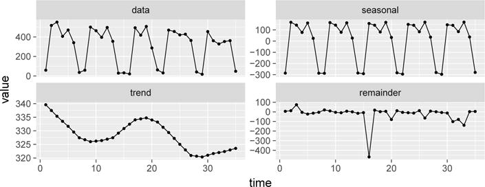
Seasonal-Trend (STL) decomposition of a time series. The top-right graph shows the original data, which has a strong (weekly) seasonality. The following graphs show the seasonal, trend, and remainder signals decomposed from the original time series. Notice the point at time 16 is an outlier.

2.3 Likelihood Ratio Statistics

Given a set of data points x = {x₁, x₂, …, x_n} within a window at time t with the seasonal signal removed, we want to derive a score indicating how likely a change in the mean has occurred in the time span [t − n + 1, t]. Ultimately, we want to know if a change has occurred or not (1 or 0), and a score is a continuous quantity representing our belief that a change has occurred. By applying a threshold to the scores, we can convert them to binary labels indicating changes.

To calculate the scores, we formulate the following hypothesis test for each possible change-point c, 1 < c ≤ n.

$$H_0:x_i\sim F\left({\mu }_0\right),1\le i\le n.H_1:x_i\sim F\left({\mu }_1\right),x_j\sim F\left({\mu }_n\right),1\le i<c\le j\le n.$$ (1)

F is a distribution family with a parameter for the mean. If we fix c, the change-point, then the likelihood ratio statistic would be

$$r_c=\log L_{H_c}-\log L_{H_0},$$ (2)

where $L_{H_0}$ is the maximum likelihood of the sample x under the null hypothesis, and $L_{H_c}$ is under the alternative hypothesis with known c. Since we do not know c, and instead want to detect whether there is a change at any point, the score for the sample x is

$$r_{\ast }=\underset{1<c\le n}{max}{r}_c,$$ (3)

and the corresponding maximizer is the suspected change-point.

The statistics depend on the distribution family F. Because the data can be quite noisy and contain outliers, we use Student’s t-distribution to model the data. Specifically, the probability density function (PDF) is

$$p(x|\nu ,\mu ,{\sigma }^2)=\frac{\Gamma \left(\frac{\nu +1}{2}\right)}{\Gamma \left(\frac{\nu }{2}\right)\sqrt{\pi \nu {\sigma }^2}}{\left(1+\frac{{\left(x-\mu \right)}^2}{\nu {\sigma }^2}\right)}^{-\frac{\nu +1}{2}},$$ (4)

where ν is the degrees of freedom, μ is the location, and σ² is the scale.

We consider ν as given and only estimate μ and σ². For t-distributions, the maximum likelihood estimators (MLEs) do not have a closed-form solution, so we follow [15] and develop an EM algorithm for estimating the parameters under either the null or the alternative hypothesis. The EM algorithm is based on an equivalent form of the distribution as an infinite mixture of Gaussians, which includes an additional hidden variable τ:

$$\tau \sim \text{Gamma}\left(\nu /2,\nu /2\right),x\sim N\left(\mu ,{\sigma }^2/\tau \right),$$ (5)

where the parameters of the Gamma distribution are shape and rate. The marginal distribution of x in Eq. 5 is the t-distribution in Eq. 4.

Based on the above, for the null hypothesis, the EM algorithm is as follows. The E-step is

$$w_i=E[{\tau }_i|x_i,\nu ,{\mu }_0,{\sigma }^2]=\frac{\nu +1}{\frac{{\left(x_i-{\mu }_0\right)}^2}{{\sigma }^2}+\nu }.$$ (6)

The M-step is

$${\mu }_0=\frac{{\displaystyle {\sum }_i{w}_i{x}_i}}{{\displaystyle {\sum }_i{w}_i}},{\sigma }^2=\frac{{\displaystyle {\sum }_i{w}_i{\left(x_i-\mu \right)}^2}}{n}.$$ (7)

We alternate between the E-step and M-step till convergence, use the final values of μ₀ and σ² as the MLEs.

For the alternative hypothesis, the E-step is almost the same as Eq. 6, except that μ₀ is replaced by μ₁ or μ_n depending on whether i < c or not. The M-step is

$$\begin{array}{l}{\mu }_1=\frac{{\displaystyle {\sum }_{i<c}{w}_i{x}_i}}{{\displaystyle {\sum }_{i<c}{w}_i}},{\mu }_n=\frac{{\displaystyle {\sum }_{i\ge c}{w}_i{x}_i}}{{\displaystyle {\sum }_{i\ge c}{w}_i}},\\ {\sigma }^2=\frac{{\displaystyle {\sum }_{i<c}{w}_i{\left(x_i-{\mu }_1\right)}^2+{\displaystyle {\sum }_{i\ge c}{w}_i{\left(x_i-{\mu }_n\right)}^2}}}{n}.\end{array}$$ (8)

2.4 Further Improvements

The data are counts, and even with transformation, low counts are problematic, because the variance is too low. To improve the performance, we add a small noise to the data. Specifically, for every point x in the time series after transformation, we add a noise as

$$x^{\prime }=x+\epsilon ,\epsilon =u-0.5,u\sim \mathit{Beta}\left(a,a\right).$$ (9)

We use a (symmetric) beta-distribution, so the size of the noise is within control, ε ∈ [−0.5, 0.5], and the mean of ε is 0.

The second improvement is based on the following observation. When calculating the likelihood ratio statistics, if say c = 2 or n, only one point is used for estimating μ₁ or μ_n, so the sample size is small. But our data contain outliers, which can bias the inference especially when the sample size is small. We can make sure the sample size is always greater than l by restricting l < c ≤ n − l + 1, but an obvious drawback is that the expected delay of the detection would increase. However, noticing that new data always come from the right of the sliding window, and usually the change can be detected quickly, we restrict l < c ≤ n instead, so the sample size for estimating μ₁ is at least l, while the delay of the detection is not affected at all, if without the restriction it would be detected within n − l observations after the change.

3 Experiments

3.1 Experiment Design

We test our framework and compare it to alternative methods on rule firing counts from a large teaching hospital collected over a period of approximately 5 years [22]. We run and evaluate the methods by considering both (1) known and (2) simulated changes in their time series.

In the first part of the experiment we use 14 CDSS rules with a total of 22 labeled change-points. These reflect known changes in the rule logic, or confirmed changes in the firing rates due to various issues. In the second part we simulate changes on the existing rule firing counts to help us analyze the sensitivity of the methods to the magnitude of the changes. We use the firing counts of 4 CDSS rules with no known change-points, and simulate change-points on these data by randomly sampling 10 segments of length 240 per rule and simulating a change in the middle of these segments. We simulate the change at time c in time series x by changing the values as $x_i^{\prime }=\lambda x_i$. i ≥ c In different experiments, we set λ to 2/1, 3/2, 6/5, 1/2, 2/3, and 5/6 respectively, to cover both increasing and decreasing changes in different sizes. The final values x_i are rounded, so they are still nonnegative integers consistent with counts. We use multiplicative instead of additive changes, because the data are counts and have heteroscedasticity.

We use AMOC curves [7] to evaluate the performance of the methods. In general, a change-point can be detected within an acceptable delay. Meanwhile, normal points can be falsely detected, resulting in false positives. In an AMOC curve, the delay of a detection is plotted against the false positive rate (FPR) by varying the threshold on the scores. If a change is not detected at all, a penalty is used as the delay. In our experiments, the maximum delay is 13, which is related to the sliding window size explained later, and the penalty is 14. The first 140 points in each time series are used as a warm-up, and no scores are produced.

We compare the following methods:

• –RND: a baseline that gives uniformly sampled scores.
• –SCP: single change-point detection method for normal distribution [13].
• –MW: a method based on Mann-Whitney nonparametric statistics [18].
• –Pois: a method based on Poisson likelihood ratios [3].
• –NDT1: our method without restricting l < c.
• –NDT2: our method with restricting l < c, where l = 7.

A window of 14 is used for change detection, while a window of 140 is for STL. The square-root transformation is also used for SCP.

We use the robust STL implemented in R [19] and set the period to 7 (a week) and s.window = 7 (even smaller values are not recommended [4]). Default values are used for other parameters. ν = 3 for Eq. 4 and 5. a = 1 for Eq. 9.

3.2 Results on Data with Known Change-Points

AMOC curves on the real data are shown in Fig. 2a. Notice that our methods dominate all the other methods almost everywhere, meaning for almost any given FPR, our methods have a lower delay in detection compared with the others. Comparing NDT1 and NDT2, we notice NDT2 is better, especially when the FPR is low, showing the effectiveness of the second improvement. We also did experiments for NDT without any improvements in Section 2.4, and the performance (not listed) is worse than NDT1.

Fig. 2.

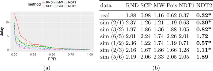
(a) AMOC curves on real data averaged over all change-points. (b) The mean AUC-AMOC averaged over all change-points. *Wilcoxon tests show that NDT2 significantly (.05) outperforms other methods.

The means of the areas under the AMOC curves (AUC-AMOC) are in Fig. 2b (row 1). These are calculated by treating the data around each change-point as a single example. For each example, the AUC summarizes the AMOC curve by integrating the delay w.r.t. the FPR. These results show that our methods are the best in terms of the overall performance.

3.3 Results on Data with Simulated Change-Points

AMOC curves on the simulated data are shown in Fig. 3. They are grouped by experiment settings, that is the fold of the simulated changes (the value of λ). Each subgraph corresponds to a different fold, shown in the label on the top. A general trend in these graphs is that, as the change gets smaller, all the curves get closer to the random baseline (RND). This reflects that the smaller the change, the harder to detect it (in time). But except when the change is at the smallest setting (the last column of the graphs), our methods dominate the other methods almost everywhere by a noticeable margin.

Fig. 3.

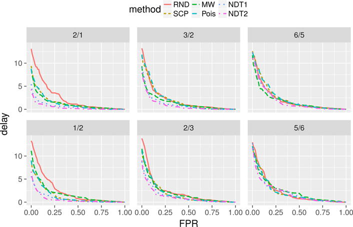
AMOC curves on simulated data averaged over all change-points. The label on top of each subgraph indicates the fold of the changes (λ).

Fig. 2b (row 2–7) shows the mean AUC-AMOC for different folds of changes (λ). NDT2 performs the best in all cases, although when λ = 6/5, 5/6, the difference is not significant.

4 Related Work and Discussion

Although change-point detection has been studied by statisticians for a long time, most work focused on offline detection. For example, Sen and Srivastava [20] study likelihood ratio test for detecting changes in mean for normal distributions. Pettitt [18] proposes a nonparametric statistics for detecting changes. Killick et al. [14] and Frizlewicz [9] improve efficiency in detecting multiple change-points. An exception is work in quality control (e.g., CUSUM [17]), where tests are performed in a sequential manner to detect errors in real time. However, these methods usually need a reference value, so it is hard to apply them to nonstationary time-series data like ours. Furthermore, all the methods assume the data are independent and identically distributed. The assumption does not hold for our data.

Research in time-series outlier detection is also related. Fox [8] defines and studies two types of outliers. Tsay [21] extends them to four types. These concepts are defined in terms of ARIMA (autoregressive integrated moving average) models. Chen and Gupta [2] improve upon the previous work by jointly estimating model parameters and outlier effects. Although some types of outliers correspond to change-points, their work has some limitations. First, they assume the model generating the time series is ARIMA. As soon as the time series do not follow ARIMA, their theoretical justifications are gone, and some algorithms may not even work properly without modifications. Second, they all deal with offline detection, so the algorithms are usually inefficient for online detection.

In the data mining community, there is some work addressing online change-point detection. Yamanishi and Takeuchi [23] propose a framework for detecting both additive outliers and change-points based on AR (autoregressive) models, which are even more restricted than ARIMA models. Therefore, they do not fit our data at all. In [12] the authors directly model the likelihood ratio with kernels, but their method needs enough data before and after the change-point, so they actually solve a different problem: they only consider a change-point to be a fixed point (say the mid-point) within a large sliding window. Therefore, the delay of the detection is always bounded below by a large number, which is not preferable in practice.

5 Conclusion

Monitoring a CDSS and detecting changes in rule firing counts can help us detect system malfunctions and reduce costs. In this work, we have developed a change-point detection method based on STL decomposition and likelihood ratio statistics, and two improvements to further boost the performance. The method can be applied efficiently to detect changes in real time. Experiments on real data with both known and simulated changes have shown that our method outperforms traditional change-point detection methods in terms of false positive rate and detection delay.

In the future we plan to test the methodology on hundreds of CDSS rules and study the feasibility of the method in detecting rule firing changes in terms of precision-alert-rate (PAR) curves [11]. In terms of the methodology, our detection methods currently work only with the time-series of rule counts and ignore context information other than the day of the week (accounted for by STL). An interesting open problem is how to add additional covariates into the change-point models that can account for other types of variations similarly to spike detection work in [16].

References

- 1.Bartlett MS. The Use of Transformations. Biometrics. 1947;3(1):39–52. [PubMed] [Google Scholar]
- 2.Chen C, Liu LM. Joint Estimation of Model Parameters and Outlier Effects in Time Series. Journal of the American Statistical Association. 1993;88(421):284–297. [Google Scholar]
- 3.Chen J, Gupta AK. Parametric Statistical Change Point Analysis. Birkhäuser; Boston, Boston: 2012. [Google Scholar]
- 4.Cleveland RB, Cleveland WS, McRae JE, Terpenning I. STL: A seasonal-trend decomposition procedure based on loess. Journal of Official Statistics. 1990;6(1):3–73. [Google Scholar]
- 5.Cleveland WS, Cleveland WS. Robust Locally Weighted Regression and Smoothing Scatterplots. Journal of the American Statistical Association. 1979 Dec;74(368):829–836. [Google Scholar]
- 6.Cleveland WS, Devlin SJ. Locally Weighted Regression: An Approach to Regression Analysis by Local Fitting. Journal of the American Statistical Association. 1988 Sep;83(403):596–610. [Google Scholar]
- 7.Fawcett T, Provost F. Activity monitoring: Noticing interesting changes in behavior. ACM SIGKDD International Conference on Knowledge Discovery and Data Mining. 1999;1:53–62. [Google Scholar]
- 8.Fox AJ. Outliers in Time Series. Journal of the Royal Statistical Society. Series B (Methodological) 1972 Jan;34(3):350–363. [Google Scholar]
- 9.Fryzlewicz P. Wild Binary Segmentation for multiple change-point detection. The Annals of Statistics. 2014;42(6):2243–2281. [Google Scholar]
- 10.Garg AX, Adhikari NKJ, McDonald H, Rosas-Arellano MP, Devereaux PJ, Beyene J, Sam J, Haynes RB. Effects of Computerized Clinical Decision Support Systems on Practitioner Performance and Patient Outcomes: A Systematic Review. JAMA. 2005 Mar;293(10):1223–1238. doi: 10.1001/jama.293.10.1223. [DOI] [PubMed] [Google Scholar]
- 11.Hauskrecht M, Batal I, Hong C, Nguyen Q, Cooper GF, Visweswaran S, Clermont G. Outlier-based detection of unusual patient-management actions: An icu study. Journal of Biomedical Informatics. 2016;64:211–221. doi: 10.1016/j.jbi.2016.10.002. [DOI] [PMC free article] [PubMed] [Google Scholar]
- 12.Kawahara Y, Sugiyama M. SIAM International Conference on Data Mining. Society for Industrial and Applied Mathematics; Apr, 2009. Change-Point Detection in Time-Series Data by Direct Density-Ratio Estimation; pp. 389–400. [Google Scholar]
- 13.Killick R, Eckley I. changepoint: An r package for changepoint analysis. Journal of Statistical Software. 2014;58(3):1–19. [Google Scholar]
- 14.Killick R, Fearnhead P, Eckley IA. Optimal detection of changepoints with a linear computational cost. Journal of the American Statistical Association. 2012;107(500):1590–1598. [Google Scholar]
- 15.Liu C, Rubin DB. ML Estimation of the t Distribution Using EM and Its Extensions, ECM and ECME. Statistica Sinica. 1995;5:19–39. [Google Scholar]
- 16.Liu S, Wright A, Hauskrecht M. Online conditional outlier detection in non-stationary time series. FLAIRS Conference. 2017 [PMC free article] [PubMed] [Google Scholar]
- 17.Page ES. Continuous Inspection Schemes. Biometrika. 1954;41(1/2):100–115. [Google Scholar]
- 18.Pettitt AN. A Non-Parametric Approach to the Change-Point Problem. Journal of the Royal Statistical Society. Series C (Applied Statistics) 1979;28(2):126–135. [Google Scholar]
- 19.R Core Team. R: A Language and Environment for Statistical Computing. R Foundation for Statistical Computing; Vienna, Austria: 2016. [Google Scholar]
- 20.Sen A, Srivastava MS. On Tests for Detecting Change in Mean. The Annals of Statistics. 1975;3(1):98–108. [Google Scholar]
- 21.Tsay RS. Outliers, Level Shifts, and Variance Changes in Time Series. Journal of Forecasting. 1988;7:1–20. (May 1987) [Google Scholar]
- 22.Wright A, Hickman TTT, McEvoy D, Aaron S, Ai A, Andersen JM, Hussain S, Ramoni R, Fiskio J, Sittig DF, Bates DW. Analysis of clinical decision support system malfunctions: A case series and survey. JAMIA. 2016 Mar; doi: 10.1093/jamia/ocw005. [DOI] [PMC free article] [PubMed] [Google Scholar]
- 23.Yamanishi K, Takeuchi JI. ACM SIGKDD International Conference on Knowledge Discovery and Data Mining. ACM; 2002. A Unifying Framework for Detecting Outliers and Change Points from Non-stationary Time Series Data; pp. 676–681. [Google Scholar]