Abstract
In this paper, we propose a novel 3D segmentation method based on the effective combination of the active appearance model (AAM), live wire (LW), and graph cut (GC). The proposed method consists of three main parts: model building, initialization, and segmentation. In the model building part, we construct the AAM and train the LW cost function and GC parameters. In the initialization part, a novel algorithm is proposed for improving the conventional AAM matching method, which effectively combines the AAM and LW method, resulting in Oriented AAM (OAAM). A multi-object strategy is utilized to help in object initialization. We employ a pseudo-3D initialization strategy, and segment the organs slice by slice via multi-object OAAM method. For the segmentation part, a 3D shape constrained GC method is proposed. The object shape generated from the initialization step is integrated into the GC cost computation, and an iterative GC-OAAM method is used for object delineation. The proposed method was tested in segmenting the liver, kidneys, and spleen on a clinical CT dataset and also tested on the MICCAI 2007 grand challenge for liver segmentation training dataset. The results show the following: (a) An overall segmentation accuracy of true positive volume fraction (TPVF) > 94.3%, false positive volume fraction (FPVF) < 0.2% can be achieved. (b) The initialization performance can be improved by combining AAM and LW. (c) The multi-object strategy greatly facilitates the initialization. (d) Compared to the traditional 3D AAM method, the pseudo 3D OAAM method achieves comparable performance while running 12 times faster. (e) The performance of proposed method is comparable to the state of the art liver segmentation algorithm. The executable version of 3D shape constrained GC with user interface can be downloaded from website http://xinjianchen.wordpress.com/research/.
Keywords: Object Segmentation, Active Appearance Models, Live Wire, Graph Cut
I. INTRODUCTION
Image segmentation is a fundamental and challenging problem in computer vision and medical image analysis. In spite of several decades of research and many key advances, a few challenges still remain in this area. Efficient, robust, and automatic segmentation of anatomy on radiological images is one of these challenges.
The image segmentation methods could be classified into several types: image based [1–12], model based [13–30], and hybrid methods [31–39]. Purely image based methods perform segmentation based only on image information; these include thresholding, region growing [1], morphological operations [2], active contours [3, 4, 22], level sets [5], live wire (LW) [6], watershed [7], fuzzy connectedness [8, 9] and graph cut (GC) [10, 11, 47]. These methods perform well on high quality images. However, the results are not as good when the image quality is inferior or boundary information is missing. In recent years, there has been an increasing interest in model-based segmentation methods. One advantage of these methods is that, even when some boundary information is missing, such gaps can be filled due to the closure and connectedness properties of the model. The model-based methods employ object population shape and appearance prior such as atlases [13–17, 23–25], statistical active shape model [18–20, 26], and statistical active appearance models (AAMs) [21, 27, 28]. MICCAI 2007 “Grand Challenge” workshop [29] organized a competition for liver segmentation which attracted a lot of attention. In that competition, the three best-rated approaches [29, 30] were all based on statistical shape models with some form of additional deformation. Such hybrid approaches are rightfully attracting a great deal of attention at present. The relative merits of the synergy that exists between these two approaches – purely image-based and model-based strategies – are clearly emerging in the segmentation field. As such hybrid methods that form a combination of two or more approaches are emerging as powerful segmentation tools [31–39] where their superior performance and robustness over each of the component methods have been well demonstrated.
Many of the above mentioned image-based [1, 4], model-based [14–18, 20–25, 30], as well as hybrid [39] techniques were tailored for specific body regions and image modalities. However, it is desirable to have a general approach that is applicable to any (or most) body regions and image modalities and protocols and not heavily dependent on the characteristics of fixed shape families and image modalities. While perhaps some of the above techniques can be generalized in this spirit, few methods have demonstrated to work in this general setting.
In this paper, we propose a general method which can be used to segment most organs and which effectively combines the AAM, LW, and GC methods, leading to the GC-OAAM approach, and arrive at an automatic, efficient, and accurate segmentation method. LW is a user-steered 2-dimensional segmentation method in which the user provides recognition help and the algorithm does the delineation precisely. The major limitation of live wire is that the recognition process (selecting anchor points on the boundary) is done by a human operator; hence it is far less efficient. AAM methods use landmarks to represent shape and appearance, and use principal component analysis to capture the major modes of variation in shape and appearance observed in the training data sets. However, the specific shape and appearance information are also lost during the model building. GC methods have the ability to compute globally optimal solutions and have proven to be a useful multidimensional optimization tool which can enforce piecewise smoothness while preserving relevant sharp discontinuities. However, some GC methods need human operator to label the source and sink seeds. In this paper, our aim is to combine the complementary strengths of the individual methods to arrive at a more powerful hybrid strategy that can overcome the weakness of the component methods.
Several existing approaches embody hybrid integration in the above spirit. Besbes et al. [12] proposed a discrete MRF based segmentation method which combined shape priors and regional statistics. However, this method did not perform segmentation at the pixel level. Freedman and Zhang [34] incorporated a shape template into the graph-cut formulation as a distance function. However, it relied crucially on user input. Based on the latter method, Ayvaci and Freedman [35] proposed a joint registration-segmentation method which removed the user interaction requirement and resolved the problem of template registration. However, this method required proper registration of the shape template for an accurate segmentation. Kumar et al. [36] used a MRF representation where the latent shape model variables were integrated via expectation maximization. While shape information was utilized in a principled Bayesian manner, this approach was computationally intensive where a separate energy minimization was required. Malcolm et al. [37] imposed the shape prior model on the terminal edges and performed graph cut optimization iteratively starting from an initial contour. Their method constructed a statistical shape space using kernel principal component analysis. This method also relied on user input. Vu and Manjunath [38] proposed a shape prior integrated segmentation method using graph cuts suitable for multiple objects. The shape prior energy was based on a shape distance popular in level set approaches. However, the shape used was a simple fixed shape. Most of the above mentioned methods operated on 2D images.
Compared to these methods, the strategy proposed in this paper is a 3D anatomy segmentation method. More importantly, different from all the above shape prior-integrated methods, our technique does not need shape registration. The proposed GC-OAAM effectively combines the rich statistical shape and appearance information embodied in AAM, effective boundary oriented delineation in LW, with the globally optimal delineation capability of the GC method.
The remaining part of this paper is organized as follows. In Section 2, we elaborate the complete methodology of the delineation algorithm. In Section 3, we describe an evaluation of this method in terms of its accuracy and efficiency. In Section 4, we summarize our contribution.
II. THE GC-OAAM APPROACH
2.1 Overview of the approach
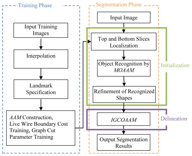
The proposed method consists of two phases: training phase and segmentation phase. Fig. 1 shows the flowchart of the proposed method. In the training phase, an AAM is constructed and the LW boundary cost function and GC parameters are trained. The segmentation phase consists of two main steps: initialization and delineation. In the initialization step, we employ a pseudo 3D initialization strategy in which the organs are initialized slice by slice via a multi-object OAAM method, and a refinement method is applied to further adjust the initialization results. The employment of pseudo 3D initialization strategy is motivated by two reasons: (1) Compared to a full 3D initialization method, the proposed method is much faster. (2) It is difficult to combine AAM with LW in 3D. The experimental results demonstrate that the proposed method has performance comparable to the full 3D AAM initialization method, which may be due to the effective combination of AAM with the LW method. Finally, for the delineation part, the object shape information generated from the initialization step is integrated into the GC cost computation. An iterative GC-OAAM method is proposed for object delineation. The details of each step are given in the following sub-sections.
Fig. 1.
The flowchart of the proposed GC-OAAM system.
2.2 Model Building and Parameter Training
Before building the model, the top and bottom slices of each organ are first manually identified. Then linear interpolation is applied to generate the same number of slices for the organ in every training image. 2D OAAM models are then constructed for each slice level from the training images. The LW cost function and GC parameters are also estimated in this stage.
2.2.1 Landmark Specification
Due to the nature of the proposed method (slice by slice), we represent a 3D shape as a stack of 2D contours, and manually label the 3D shape slice by slice, although semi-automatic or automatic methods are also available for this purpose. For each slice, operators locate the shape visually, and then identify prominent landmarks on that shape.
2.2.2 AAM Construction
The standard AAM method [27, 28] is used to construct the model. The model includes both shape and texture information.
The generative model can be described by
| (1) |
where Q is a matrix of the selected eigenvectors of the covariance matrix over the training samples for shape and texture, b is the model parameter vector and x is a sample generated by the model.
Suppose Mj represents the AAM for slice level j and the number of slice levels is n, then the overall model M can be represented as
| (2) |
Although we employ the pseudo 3D initialization strategy, we also build the real 3D AAM M3D using the method in [43]. However, this 3D model M3D is used only for providing the delineation constraints as to be explained later.
2.2.3 LW Cost function and GC Parameter Training
Similar to the OASM method [31], an oriented boundary cost function is devised for each organ in the model M as per live wire method [6].
A boundary element, bel for short, of a given image slice I is an ordered pair (a, b) of 4-adjacent pixels a and b. It represents the oriented edge between pixels a and b, (a, b) and (b, a) representing its two possible orientations. To every bel of I, we assign a set of features. The features are intended to express the likelihood of the bel belonging to the boundary (of a particular object) that we are seeking in I. The cost c(b) associated with each bel b of I is a linear combination of the costs assigned to its features
| (3) |
where wi is a positive constant indicating the emphasis given to feature function fi, and cf is the function to convert feature values fi (b) at b to cost values cf (fi (b)). In live wire technique [6], fi represents features such as intensity on the immediate interior of the boundary, intensity on the immediate exterior of the boundary, and gradient magnitude at the center of the bel. cf is an inverted Gaussian function, and here, uniform weights wi are used for all selected features.
For the purpose of OAAM, we shall utilize the feature of live wire to define the best oriented path between any two points as a sequence of bels with minimum total cost. The only deviation in this case is that the two points will be taken to be any two successive landmarks employed in the AAM, and the landmarks are assumed to correspond to pixel vertices. With this facility, we assign a cost to every pair of successive landmarks of any shape instance x associated with Mj, which represents the total cost of the bels in the best
oriented path <b1, b2,.…, bh> from landmark xk to landmark xk+1. That is,
| (4) |
For any shape instance x = (x1, x2,…, xn) of Mj, the cost structure K(x) associated with Mj may now be defined as
| (5) |
where m is the number of landmarks for this slice and we assume that xm+1 = x1. That is, K(x) is the weighted sum of the costs associated with the best oriented paths between all m pairs of successive landmarks of shape instance x. The parameters of GC are also trained during the training stage; more details on this are given at section 2.4.1.
2.3 Initialization
The initialization step plays a key role in our method, which provides the shape constraints to the later GC segmentation step and makes it fully automatic. The proposed initialization method includes three main steps. First, a slice localization method is applied to detect the top and bottom slices of the organ. Second, a linear interpolation is applied to generate the same number of slices for the subject as in the model. And third, the organ is recognized slice by slice via the OAAM method. A multi-object strategy [44] is utilized to help with object initialization. We found from experiments that the initialization performance with multiple organs in the model is much better than with a single organ due to the constraints among multiple organs. It means that, even if just one organ is to be segmented, other organs can be employed in the segmentation to provide context and constraints. Finally, a refinement method is applied to the initialization result. These three steps are described below.
2.3.1 Top and Bottom Slices Localization
There are several recent works related to slice localization. Haas et al. [39] introduced an approach for creating a navigation table using eight landmarks which were detected in various fashions. Seifert et al. [19] proposed a method to detect invariant slices and single point landmarks in full body scans by using probabilistic boosting tree (PBT) and Haar features. Emrich et al. [40] proposed a CT slice localization method via k-NN instance based regression. The aim of slice localization in our approach is to locate the top and bottom slices of the organ. Since we already trained the model for each organ slice, we could use this model for slice localization. The proposed method is based on the similarity to the OAAM model of the slice.
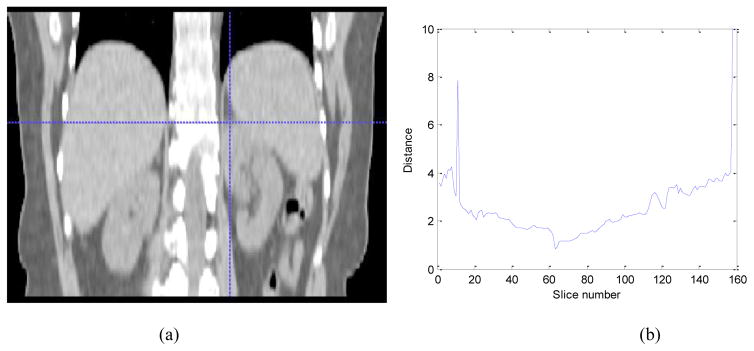
For top slice localization in a given image, the top slice model is applied to each slice in the image using the recognition method detailed in 2.3.2 and evaluating the respective similarity metric (Eqn. (6)). Then the slice corresponding to the maximal similarity (minimal distance) is taken as the top slice of the organ. Fig. 2 shows the distance value computed from Eqn. (6) for the top slice in a patient abdominal CT image. The minimum corresponds to the top slice of the left kidney. A similar method is used for the bottom slice detection.
Fig 2.
Illustration of top slice recognition. (a) Coronal view of the abdominal region. Cross point represents the top slice of the left kidney. (b) The distance values for the top slice of the left kidney.
2.3.2 Object Recognition
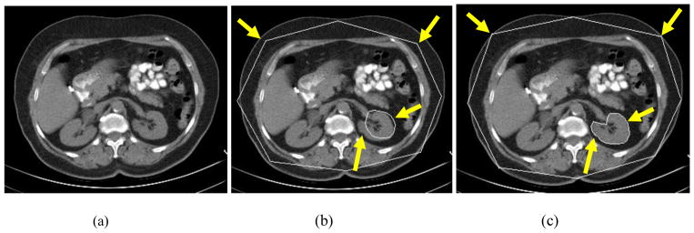
The proposed object recognition method is based on the AAM. The conventional AAM matching method for object recognition is based on the root-mean-square difference between the appearance model instance and the target image. Such a strategy is better suited for matching appearances than for the detailed segmentation of target images (see Fig. 3(b)). This is because the AAM is optimized on global appearance, and is thus, less sensitive to local structures and boundary information. Conversely, the LW delineates the boundary very well [6], however it needs good initialization of landmarks and is an interactive method. Here, we integrate the AAM with the LW method (termed OAAM) to combine their complementary strengths. That is, the AAM provides the landmarks to the LW, and as a return, LW improves the shape model of the AAM. The LW is fully integrated with AAM in two aspects: (1) LW is used to refine the shape model in AAM; (2) the LW boundary cost is integrated into cost computation during the AAM optimization method. Fig. 3(c) shows the proposed OAAM segmentation result; compared to conventional AAM method (Fig. 3(b)), the boundary delineation is much improved.
Fig. 3.
Comparison of conventional AAM and OAAM segmentation. (a) Original image. (b) Conventional AAM segmentation showing a good appearance fit but poor boundary detection accuracy (arrows). (c) OAAM result shows substantial improvement in boundary location (arrows).
2.3.2.1 Refinement of the Shape Model in AAM by LW
First, the conventional AAM searching method is performed once to obtain a rough placement of the model. Then the following method is applied to refine the shape model in AAM. The shape is extracted from the shape model of the AAM, and then the landmarks are updated based on LW using only the shape model and the pose parameters (translation, rotation and scale). Subsequently, the refined shape model is transformed back into the AAM. At the same time, AAM refinement is applied to the image yielding its own set of coefficients for shape and pose.
Suppose P1, P2 and P3 are three successive landmarks in shape instance x.
Algorithm: Refine AAM shape model based on LW
begin
Extract the shape instance x from the shape model.
-
Update the landmarks’ position in x based on LW as follows (see Fig. 4).
First, perform LW delineation from P1 to P2, and P2 to P3.
Next, find the middle point Q1 and Q2 in the LW segments generated from P1 to P2, and from P2 to P3, respectively. Then perform LW delineation from Q1 to Q2.
Finally, find the closest point P2′ on the LW segment from Q1 to Q2. Update P2 to P2′.
Perform the above three steps on all landmarks in x, and produce the updated shape model x′.
Transform x′ into a new shape model instance xa ′ via an affine transformation so as to align it with the mean shape x̄.
Apply the model constraints to the new shape model xa ′ so that the new shape is within the allowed shape-space.
Fig. 4.
The illustration of how to update the landmark’s position. (a) P1, P2 and P3 are three landmarks from AAM shape results. (b) The middle point Q1 of the LW segment between P1 and P2, Q2 of P2 and P3 are generated. (c) Landmark P2 is moved to the closest point P2′ on the live wire segment from Q1 to Q2.
end
2.3.2.2 OAAM Optimization
In the conventional AAM matching method, the optimization is based only on the difference between the appearance model instance and the target image. The boundary cost is not taken into consideration. By combining the boundary cost, the performance of AAM matching can be considerably improved. In the proposed method, the LW technique is integrated into the cost computation during the optimization process. Combined with the above shape model refinement method, our optimization method is as follows.
Algorithm OAAM Optimization
begin
Let the current estimate of the model parameter vector be b, the pose t, the texture transformation Tu and the image sample (as a vector) at the current estimate be gim.
Extract the shape parameters bs from the entire model parameter b, and refine bs and pose t using the shape refinement method described above. This results in a new set of parameters and t′.
Resample the image intensity, resulting in the vector , and project the texture sample into the texture model frame using .
Evaluate the error vector, , and the current error, Eaam =|r|2.
- Compute the live wire cost along the shape boundary, Elw, and compute the total error as
(6) Compute the predicted displacements, δb =−Rr(b), where .
Update the model parameters b ↑b + kδb, where initially k = 1.
Calculate the new shape points x, and refine the new shape using the shape refinement method described above, and obtain the refined new shape point x′.
Calculate the model frame texture , and sample the image at the new points x′ to obtain .
Calculate a new error vector, , and the error .
Compute the live wire cost along the predicted shape boundary, . And compute the total error, .
If , then accept the new estimate; otherwise, try at k = 0.5, k = 0.25, etc, until no improvement can be made.
end
In our implementation, we set α1 = α2 = 0.5. During the initialization, we employ a multi-resolution strategy, in which we start at a coarse resolution and iterate to convergence at each level before starting the next level. This strategy is more efficient than searching at a single resolution and can lead to a convergence to the correct solution even when the initial model position is away from the real object(s).
2.3.2.3 Refinement of the 3D Recognized Shapes
After objects are recognized in all slices, the recognized shapes are stacked together to form 3D objects. We observed from experiments that sometimes the initialization result for one slice is far away from the results for its neighboring slices. This signals failure of recognition for this slice. We found that at most two slices failed in recognition in this sense for each subject in all of our experiments (in 80 cases, non-failed: 71; 1 slice failed: 7; 2 slices failed: 2). When failure occurs, we interpolate the new shape from the shapes in neighboring slices. Fig. 5 shows an illustration for the proposed method. The following method is applied to improve the recognized shape results.
Fig 5.
Illustration of refinement of the 3D recognized shape
Algorithm: Refinement of the 3D recognized shape
begin
for each slice level j, 1 ≤ j ≤ n, do
Suppose the error in recognition (Eqn. (6)) for the current slice is e, and emax represents maximum error. Compute the distance dj−1 and dj+1 between the centroids of the shapes in neighboring slices j−1 and j+1.
-
Compute the total reliability for slice j as
(7) where η1, η2 and η3 are weights (in our implementation, η1=0.5, η2=0.25 and η3=0.25).
μ(dj−1), var(dj−1), μ(dj+1) and var(dj+1) are the mean and variance of dj−1 and, dj+1, respectively, which are estimated from training images during the model building process. For the first and last slice, only one neighbor slice is used.
If relj > threj, then the recognized result is considered reliable; otherwise the recognized result is discarded and the new shape is interpolated from the neighboring slices. threj is the threshold of reliability, which is also estimated from the training images.
endfor
end
2.4 Segmentation/Delineation
The purpose of this step is to precisely delineate the shapes recognized in the previous step. We propose an iterative GC-OAAM (named IGC-OAAM) method for the organ’s delineation. The GC-OAAM algorithm effectively integrates the shape information with the globally optimal 3D delineation capability of the GC method.
2.4.1 Shape integrated GC
GC segmentation can be formulated as an energy minimization problem such that for a set of pixels P and a set of labels L, the goal is to find a labeling f: P → L that minimizes the energy function En(f).
| (8) |
where Np is the set of pixels in the neighborhood of p, Rp (fp) is the cost of assigning label fp ∈ L to p, and Bp, q (fp, fq) is the cost of assigning labels fp, fq ∈ L to p and q. In two-class labeling, L = {0, 1}, the problem can be solved efficiently with graph cuts in polynomial time when Bp, q is a submodular function, i.e., Bp, q(0, 0) + Bp, q(1, 1) ≤ Bp, q(0, 1) + Bp, q(1, 0) [11].
In our framework, the unary cost Rp (fp) is the sum of a data penalty Dp (fp) and a shape penalty Sp (fp) term. The data term is defined based on the image intensity and can be considered as a log likelihood of the image intensity for the target object. The shape prior term is independent of image information, and the boundary term is based on the gradient of the image intensity.
The proposed shape-integrated energy function is defined as follows:
| (9) |
where α, β, γ are the weights for the data term, shape term Sp, and boundary term, respectively, satisfying α + β + γ=1. These components are defined as follows:
| (10) |
| (11) |
and
| (12) |
where Ip is the intensity of pixel p, object label is the label of the object (foreground). P(Ip | O) and P(Ip | B) are the probability of intensity of pixel p belonging to object and background, respectively, which are estimated from object and background intensity histograms during the training phase (details given below). d(p, q) is the Euclidian distance between pixels p and q, and σ is the standard deviation of the intensity differences of neighboring voxels along the boundary.
| (13) |
where d (p, xO) is the distance from pixel p to the set of pixels which constitute the interior of the current shape xo of object O. (Note that if p is in the interior of xo, then d (p, xO)= 0.) rO is the radius of a circle that just encloses xo. The linear time method in reference [42] was used in this paper for computing this distance.
During the training stage, the histograms of intensity for each object are estimated from the training images. Based on this, P(Ip | O) and P(Ip | B) can be computed. As for parameters α,β and γ in Eqn. (9), since α+β+γ=1, we estimate only α and β by optimizing accuracy as a function of α and β and set γ = 1−α−β. We use the gradient descent method for the optimization. Let Accu(α,β) represent the algorithm’s accuracy (here we use the true positive volume fraction [45]), α and β are initialized to 0.35 each, then Accu(α,β) is optimized over the training data set to determine the best α and β.
2.4.2 Minimizing En with Graph Cuts
Let G be a weighted graph (V, A), where V is a set of nodes, and A is a set of weighted arcs. Given a set T ⊆ V of k terminal nodes, a cut is a subset of edges C ⊆ A such that no path exists between any two nodes of T in the residue graph (V, A\C). In our implementation, we segment the object using the α-expansion method in [46].
The graph is designed as follows. We take V = P ∪ L, i.e., V contains all the pixel nodes and terminals corresponding to the labels in L which represent objects of interest plus the background. A = AN ∪ AT, where AN is the n-links which connect pixels p and q (p ∈P, q ∈ Np) and with a weight of wpq. AT is the set of t-links which connect pixel p and terminals ℓ ∈ L and with a weight of wpℓ. The desired graph with cut cost |C| equaling En(f) is constructed using the following weight assignments:
| (14) |
| (15) |
where K is a constant large enough to make the weights wpℓ positive.
2.4.3 IGC-OAAM
We assume that the recognized shapes are sufficiently close to the actual boundaries in the given image to be segmented. The IGC-OAAM algorithm then determines what the new position of the landmarks of the objects represented in the initialized shape xin should be such that the minimum graph cut cost is achieved, as presented below.
Algorithm IGC-OAAM
Input: Initialized shapes xin.
Output: Resulting shapes xout and the associated object boundaries.
begin
while number of iterations < nIteration do
Perform GC segmentation using Eqn. (9) based on the OAAM initialized shapes xin;
Compute the new position of the landmarks by moving each landmark in xin to the point closest on the GC boundary; call the resulting shapes xnew;
-
If no landmarks move, then, set xnew as xout and stop;
Else, subject xnew to the constraints of model M3D, and call the result xin.
endwhile
Perform one final GC segmentation based on xout, and obtain the associated object boundaries.
end
In our implementation, nIteration is set as 3. Also we limit the distance a landmark can move within any iteration to 6 voxels.
III. EXPERIMENTAL RESULTS
The proposed methods were tested on a clinical CT dataset. This dataset contained images pertaining to 20 patients (10 male and 10 female, ages 32 to 68), acquired from pre-contrast phase of two different type of CT scanner (GE Medical systems, LightSpeed Ultra, and Philips, Mx8000 IDT 16). The pixel size varied from 0.55 to 1 mm, and slice thickness from 1 to 5 mm. Four experiments of liver, left kidney, right kidney and spleen segmentation were done to evaluate the proposed method. All objects were manually segmented by two experts to generate the reference segmentations (ground truth). The leave-one-out strategy was used in the evaluation.
3.1 Evaluation of the Localization of the Top and Bottom Slice
The proposed slice localization method was used to detect the top and bottom slices of the liver, left kidney, right kidney and spleen. These organs were manually checked to generate the reference standard of the top and bottom position. Table 1 shows the experimental results. We observe that the localization of the top slice of liver is most accurate which may be due to the high contrast in the lung region; while the localization of liver bottom has the largest error which may be due to the lack of sufficient contrast in that region. The average localization error is 7.3 mm. Compared to Emrich et al’s result [40] of 4.5 cm, the proposed method seems superior.
Table 1.
Slice localization error (in mm) of the organ top and bottom
| Organ | Mean error (in mm) ± std.dev. | |
|---|---|---|
| Liver | Top | 5.1±2.5 |
| Bottom | 9.2±5.1 | |
| Left kidney | Top | 7.5±5.2 |
| Bottom | 6.2±4.6 | |
| Right kidney | Top | 8.3±6.5 |
| Bottom | 7.1±5.8 | |
| Spleen | Top | 8.1±5.2 |
| Bottom | 7.3±6.1 | |
| Average | 7.3±5.1 | |
3.2 Evaluation of Initialization
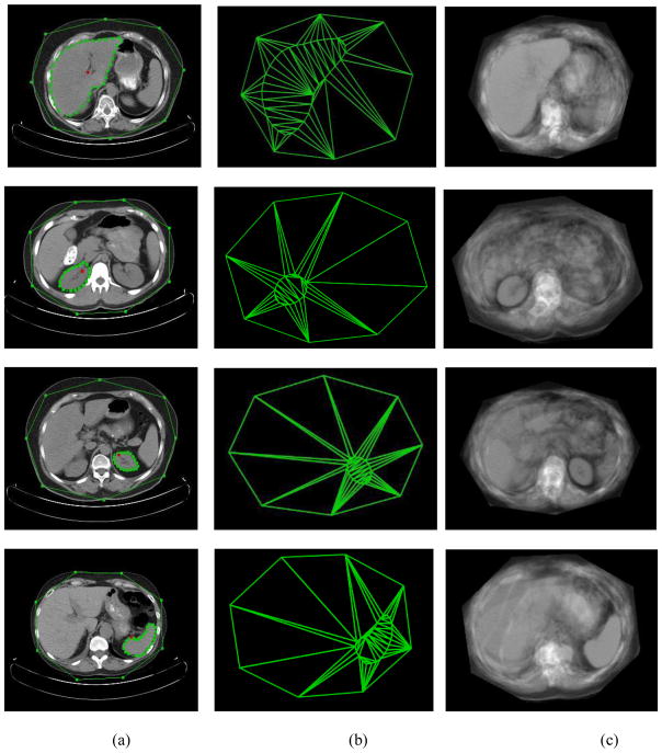
For helping with the initialization of liver, left and right kidneys, and spleen, the skin object is included in the model in addition to the object of interest. Fig. 7 shows one slice example and its corresponding mean shape and texture model for the four objects. We select only 8 landmarks for the skin object because LW works very well for this object even for such a small number of landmarks. Table 2 summarizes the number of interpolated slices and the number of landmarks used in our experiments.
Fig. 7.
Illustration of models used in organ initialization. The 1st, 2nd, 3rd and 4th row correspond to liver, right kidney, left kidney, and spleen, respectively. (a) The landmarks of organ and skin on one slice. (b) The corresponding AAM shape model for this slice level. (c) The corresponding AAM appearance model for this slice level.
Table 2.
Number of Landmarks and Slices Used in Modeling
| Number of Landmarks in Organ | Number of Landmarks in Skin Object | Number of Interpolated Slices | |
|---|---|---|---|
| Liver | 35 | 8 | 50 |
| Left Kidney | 20 | 8 | 32 |
| Right Kidney | 20 | 8 | 32 |
| Spleen | 26 | 8 | 32 |
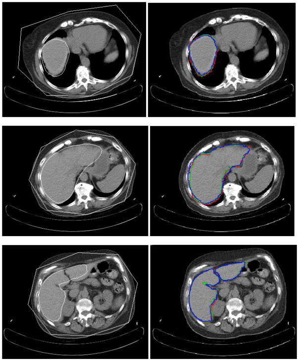
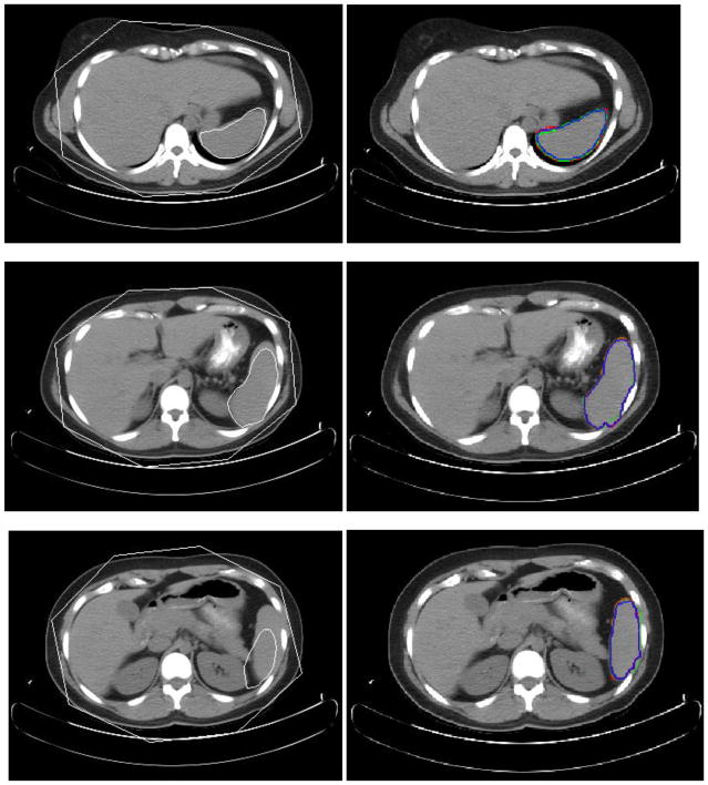
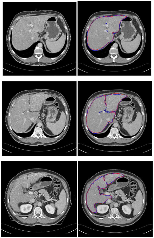
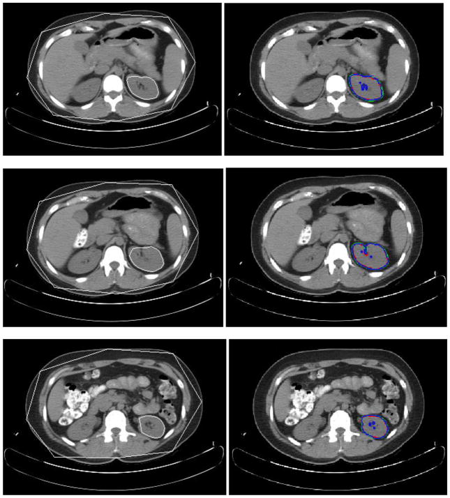
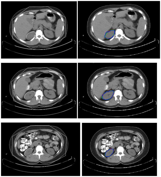
In Figs. 8–11, the left column shows sample initialization results for the four objects. A quantitative evaluation of the initialization approach is presented in Table 3. The accuracy in terms of true positive and false positive volume fractions (TPVF and FPVF) [45] is shown. TPVF indicates the fraction of the total amount of tissue in the true delineation; FPVF denotes the amount of tissue falsely identified, which are defined as follows,
Fig. 8.
Experimental results for three slice levels of liver segmentation. The left column is the MOAAM initialization result; the right is IGC-OAAM result in which red contour represents the reference image 1, green represents the reference image 2, and blue contour represents segmentation by the proposed method.
Fig. 11.
Experimental results for three slice levels of spleen segmentation. The left column is the MOAAM initialization result; the right is IGC-OAAM result in which red contour represents the reference image 1, green represents the reference image 2, and blue contour represents segmentation by the proposed method.
Table 3.
Mean and standard deviation of TPVF, FPVF for Pseudo-3D AAM, Pseudo-3D MAAM, 3D MAAM, Pseudo-3D MOAAM, and IGC-OAAM for liver, two kidneys, and spleen.
| TPVF (%) | FPVF (%) | Average Surface Dist (mm) | ||||||||||
|---|---|---|---|---|---|---|---|---|---|---|---|---|
| liver | left kidney | right kidney | spleen | liver | left kidney | right kidney | spleen | liver | left kidney | right kidney | spleen | |
| Pseudo-3D AAM | 60.01 ±5.12 | 51.01 ±8.36 | 53.01 ±6.35 | 59.31 ±7.25 | 10.12 ±2.38 | 15.36 ±3.25 | 12.15 ±3.01 | 14.62 ±4.35 | 12.12 ±5.32 | 11.59 ±4.39 | 10.98 ±4.78 | 11.32 ±4.12 |
| Pseudo-3D | 85.02 ±1.32 | 84.03 ±1.60 | 83.18 ±1.68 | 85.73 ±1.35 | 1.12 ±0.38 | 0.93 ±0.45 | 1.75 ±0.46 | 1.02 ±0.67 | 4.59 ±3.81 | 4.21 ±3.36 | 4.39 ±3.61 | 4.12 ±3.28 |
| MAAM 3D MAAM | 90.52 ±0.93 | 90.15 ±1.01 | 90.36 ±1.52 | 91.32 ±0.88 | 0.46 ±0.11 | 0.55 ±0.12 | 0.59 ±0.13 | 0.67 ±0.16 | 2.01 ±1.21 | 1.82 ±1.06 | 1.72 ±0.98 | 1.61 ±0.88 |
| Pseudo-3D MOAAM | 90.12 ±1.13 | 89.32 ±1.22 | 89.52 ±1.63 | 90.65 ±1.51 | 0.53 ±0.05 | 0.67 ±0.06 | 0.62 ±0.11 | 0.71 ±0.13 | 1.93 ±1.03 | 1.62 ±0.92 | 1.81 ±1.25 | 1.73 ±1.03 |
| Second rater | 94.86 ±0.87 | 95.32 ±0.96 | 95.12 ±0.79 | 95.22 ±1.10 | 0.12 ±0.05 | 0.15 ±0.03 | 0.16 ±0.02 | 0.12 ±0.02 | 0.79 ±0.35 | 0.71 ±0. 28 | 0.75 ±0.29 | 0.75 ±0.22 |
| IGC-OAAM | 94.03 ±0.92 | 94.15 ±1.05 | 94.35 ±0.89 | 94.68 ±1.39 | 0.16 ±0.03 | 0.13 ±0.02 | 0.21 ±0.03 | 0.15 ±0.02 | 0.81 ±0.32 | 0.75 ±0. 25 | 0.79 ±0.33 | 0.76 ±0.29 |
| (16) |
| (17) |
Where, Ud is assumed to be a binary scene with all voxels in the scene domain C set to have a value 1, as shown in Fig. 6, more details can seen in [45].
Fig. 6.
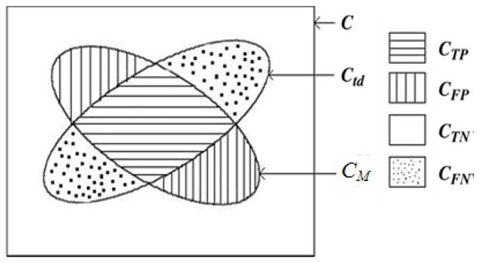
Illustration of the accuracy factors for delineation for a binary case. Here, Ctd is the corresponding scene of ‘true’ delineation, CM is the delineation result by method M.
Experiments were done to compare the performance of pseudo-3D AAM (single object, here pseudo-3D means slice-by-slice), pseudo-3D MAAM (multi-object), real 3D MAAM (multi-object), and the proposed pseudo-3D multi-object OAAM using reference images from expert #1 as ground truth. We note that the multi-object strategy improves the accuracy considerably over single object AAM. The MOAAM method also improves the MAAM initialization performance due to the effective combination of AAM and LW. The pseudo-3D MOAAM and the real 3D MAAM methods [43] have comparable performance, while the pseudo-3D MOAAM method is about 12 times faster (see Table 4). This is one of the reasons that we used the pseudo-3D initialization method.
Table 4.
Average computational time (in seconds) in all experiments for pseudo-3D MAAM, 3D MAAM, pseudo-3D MOAAM, and IGC-OAAM.
| Organ | Average computational time (in seconds) | |||
|---|---|---|---|---|
| Pseudo-3D MAAM | 3D MAAM | Pseudo-3D MOAAM (initialization) | IGC-OAAM (delineation) | |
| Liver | 50 | 732 | 60 | 310 |
| Left Kidney | 33 | 495 | 40 | 275 |
| Right Kidney | 32 | 476 | 40 | 260 |
| Spleen | 35 | 556 | 45 | 280 |
After object recognition for all the slices, all the recognized shapes are stacked together to form a 3D shape. Then the refinement of shape method proposed in section 2.3.3 is applied if the 3D shape is not transiting smoothly. We found actually our OAAM recognition method works very well and the refinement only applied to very few cases. In total 80 (20×4) cases of organ recognition, there are 7 cases with one slice of object recognition failed (liver:3, left kidney:1, right kidney:2 and spleen:1), 2 cases with two slices of object recognition failed (liver:1 and right kidney 1).
3.3 Evaluation of the IGC-OAAM Delineation Method
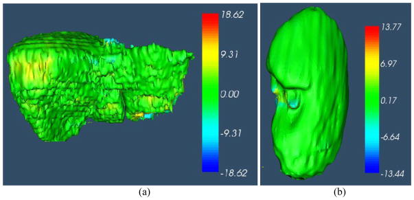
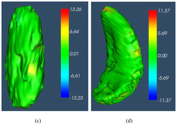
The accuracy of delineation by IGC-OAAM expressed in TPVF, FPVF and average symmetric surface distance [29] using reference images from expert #1 are summarized in Table 3. And the evaluation of the reference image from expert 1 to the reference image from expert 2 is also shown in Table 3 as the second rater. We observe that the average TPVF and FPVF is about 94.3% and 0.15%, respectively. In Figs. 8–11, the right column shows the IGC-OAAM segmentation results for the liver, left kidney, right kidney, and spleen, respectively. Additionally, Fig. 12 shows the 3D surface distance between the segmentation result by IGC-OAAM and reference image (from expert 1) for the liver, left kidney, right kidney, and spleen segmentation, respectively. The mean distance, over all objects and the whole dataset, between the segmented 3D surface and the reference (true) surface was found to be about 0.78 mm.
Fig. 12.
3D surface distance (mm) between the segmentation result by IGC-OAAM and reference image (ground truth 1). Positive value represents the vertex on the surface of the segmentation is outside of the surface of ground truth, vice versa. (a), (b), (c) and (d) correspond to surface distance for liver, right kidney, left kidney and spleen segmentation, respectively.
In terms of efficiency, Table 4 shows the computation time for the four objects on an Intel Xeon E5440 workstation with 2.83GHz CPU, 8 GB of RAM. The average total time (initialization + segmentation) for segmenting one liver is about 310 seconds. Segmentation of kidney and spleen has similar computational time, about 270 seconds.
The proposed IGC-OAAM delineation method was also tested on the MICCAI 2007 grand challenge training dataset using leave-one-out strategy. There are 20 CT volumes of abdomen with contrast agent in the training datasets. All datasets have an in-plane matrix of 512 × 512 pixels and inter-slice spacing from 0.7 mm to 5.0 mm. Fig. 13 shows the recognition and delineation results for three slice levels of one image on MICCAI grand challenge dataset..
Fig. 13.
Experimental results for three slice levels of one image on MICCAI grand challenge dataset. The left column is the MOAAM initialization result; the right is IGC-OAAM result in which red contour represents the reference (ground truth) and blue contour represents segmentation by the proposed method.
The proposed method was evaluated based on the MICCAI 2007 grand challenge for liver segmentation evaluation criteria [29]: volumetric overlap error (Overlap Error), volume difference, symmetric average surface distance, symmetric RMS surface distance, and maximal surface distance. The results achieved by the proposed method and previous work from literature are summarized in Table 5. Compare to the best performance (Kainmüller et. al [30]), we can see we have comparable performance, but much faster speed (6 min vs 15 min).
Table 5.
Comparison with other methods on MICCAI 2007 liver segmentation grand challenge
| Method | Runtime [min] | Overlap Error [%] | Volume difference [%] | Avg. distance [mm] | RMS distance | Max distance [mm] |
|---|---|---|---|---|---|---|
| Kainmuller et al. | 15 | 6.1±2.1 | −2.9±2.9 | 0.9±0.3 | 1.9±0.8 | 18.7±8.5 |
| Heimann et al. | 7 | 7.7±1.9 | 1.7±3.2 | 1.4±0.4 | 3.2±1.3 | 30.1±10.2 |
| Proposed IGC-OAAM method | 6 | 6.5±1.8 | −2.1±2.3 | 1.0±0.4 | 1.8±1.0 | 20.5±9.3 |
IV. CONCLUSIONS AND DISCUSSIONS
In this paper, we proposed a 3D automatic anatomy segmentation method. The method effectively combines the AAM, LW, and GC methods to exploit their complementary strengths. It consists of three main parts: model building, initialization, and segmentation. For the initialization part, we employ a pseudo-3D strategy, and segment the organs slice by slice via multi-object OAAM method which effectively combines the AAM and LW methods. For the segmentation (delineation) part, an iterative GC-OAAM method is proposed which integrates the shape information gathered from initialization with a GC algorithm. The method was tested on a clinical CT dataset with 20 patients for segmenting the liver, kidneys, and spleen. The experimental results suggested that an overall segmentation accuracy of TPVF > 94.3%, FPVF < 0.2% can be achieved.
As for the initialization, we employed a pseudo-3D strategy and combined AAM and LW methods to improve the performance. The multi-object strategy also helped initialization due to increased constraints. Compared to the real 3D AAM method, the pseudo 3D OAAM approach has comparable accuracy while has roughly a 12-fold speed up. The purpose of initialization is to provide a rough object localization and shape constraints for latter GC method which will produce refined delineation. We think it is better to have a fast and robust method than a slow and more accurate technique for initialization.
As for the delineation, shape constrained GC method is the core part of the whole system. Several similar ideas were also proposed in the references [34–38]. However, they are mostly tested in the 2D images, and it is difficult to compare with these methods because the testing dataset is different.
From Figs. 8–11 and the testing result in table 5, it seems that the proposed method was a little bit under-segmenting the organ. This may due to two reasons: (1) the shape term designed in our cost function is not symmetric. We didn’t put the penalty for the pixel if it is inside the shape. That is because we found there are usually some pixels which don’t belong to the target organ inside the shape, such as urine in the kidney (Fig. 10). So our method can separate this kind of pixels out. We think this is the beauty of our method. (2) according to our experiences, the expert is easily tender to over-segmenting the organ during the process of manually segmenting the boundaries.
Fig. 10.
Experimental results for three slice levels of left kidney segmentation. The left column is the MOAAM initialization result; the right is IGC-OAAM result in which red contour represents the reference image 1, green represents the reference image 2, and blue contour represents segmentation by the proposed method.
Although localizing a CT slice within a human body can greatly facilitate the workflow of a physician, so far, this area of research has not received much attention. The proposed slice localization method aims to localize the top and bottom slices of organs, which is important part of the whole system. The average localization error over the whole dataset and all organs is only about 7.3 mm (much improved compared to the result of 4.5 cm in [40]), good for clinical use. In a similar manner, it can also be used to localize any slice by constructing the corresponding slice model.
In this paper, only one object is segmented at a time. With the shape constraints of multiple organs, the proposed IGC-OAAM method can be easily generalized to segment multiple organs simultaneously. However, this brings up an issue for GC - of the unavailability of a globally optimal min cut solution for simultaneously segmenting multiple objects. For single object segmentation, global optimality is guaranteed. For multiple objects, the α-expansion method can find segmentations only within a known factor of the global optimum [46].
Current proposed method for segmenting one organ is taking about 5 min. To make it more realistic in clinical application, the parallelization or multi-threads of the algorithm is one of the good solutions. Anderson et al. [48] and Liu et al. [49] proposed the parallelization of GC methods, and achieved the good performance. This will also be investigated for the proposed method in near future.
The executable version of 3D shape constrained GC with user interface can be downloaded from website http://xinjianchen.wordpress.com/research/. Source codes will be available soon. By opening source, we believe it will benefit to the whole society.
Fig. 9.
Experimental results for three slice levels of right kidney segmentation. The left column is the MOAAM initialization result; the right is IGC-OAAM result in which red contour represents the reference image 1, green represents the reference image 2, and blue contour represents segmentation by the proposed method.
Acknowledgments
This research was supported in part by the Intramural Research Program of the NIH, Clinical Center.
References
- 1.Ruskó L, Bekes G, Németh G, Fidrich M. Fully automatic liver segmentation for contrast-enhanced CT images. Proc. MICCAI Workshop 3-D Segmentat. Clinic: A Grand Challenge; 2007. pp. 143–150. [Google Scholar]
- 2.Kaneko T, Gu L, Fujimoto H. Recognition of Abdominal Organs Using 3D Mathematical Morphology. Systems and Computers in Japan. 2002;33(8):75–83. [Google Scholar]
- 3.Kass M, Witkin A, Terzopoulos D. Snakes: Active contour models. International Journal of Computer Vision. 1987;1: 321–331. [Google Scholar]
- 4.Liu F, Zhao B, Kijewski PK, Wang L, Schwartz LH. Liver segmentation for CT images using GVF snake. Medical Physics. 2005;32(12):3699–3706. doi: 10.1118/1.2132573. [DOI] [PubMed] [Google Scholar]
- 5.Malladi R, Sethian JA, Vemuri BC. Shape Modeling with Front Propagation: A Level Set Approach. IEEE Trans Pattern Analysis and Machine Intelligence. 1995;17(2):158–175. [Google Scholar]
- 6.Falcao AX, Udupa JK, Samarasekera S, Sharma S. User-Steered Image Segmentation Paradigms: Live Wire and Live Lane. Graphical Models and Image Processing. 1998;60: 233–260. [Google Scholar]
- 7.Grau V, Mewes AUJ, Alcañiz M, Kikinis R, Warfield SK. Improved watershed transform for medical image segmentation using prior information. IEEE Transactions on Medical Imaging. 2004;23(4):447–458. doi: 10.1109/TMI.2004.824224. [DOI] [PubMed] [Google Scholar]
- 8.Udupa JK, Samarasekera S. Fuzzy connectedness and object definition: Theory, algorithms, and applications in image segmentation. Graphical Models and Image Processing. 1996;58(3):246–261. [Google Scholar]
- 9.Udupa JK, Saha PK, Lotufo RA. Relative fuzzy connectedness and object definition: Theory, algorithms, and applications in image segmentation. IEEE Transactions on Pattern Analysis and Machine Intelligence. 2002;24:1485–1500. [Google Scholar]
- 10.Boykov Y, Kolmogorov V. An Experimental Comparison of Min-Cut/Max-Flow Algorithms. IEEE Trans Pattern Analysis and Machine Intelligence. 2004;26(9):1124–1137. doi: 10.1109/TPAMI.2004.60. [DOI] [PubMed] [Google Scholar]
- 11.Kolmogorov V, Zabih R. What Energy Functions can be Minimized via Graph Cuts? IEEE Trans Pattern Anal Mach Intell. 2004;26(2):147–159. doi: 10.1109/TPAMI.2004.1262177. [DOI] [PubMed] [Google Scholar]
- 12.Besbes A, Komodakis N, Langs G, Paragios N. Shape priors and discrete MRFs for knowledge-based segmentation. CVPR. 2009;2009:1295–1302. [Google Scholar]
- 13.Park H, Bland P, Meyer C. Construction of an Abdominal Probabilistic Atlas and Its Application in Segmentation. IEEE Transactions on Medical Imaging. 2003;22(4):483–492. doi: 10.1109/TMI.2003.809139. [DOI] [PubMed] [Google Scholar]
- 14.Cuadra MB, Pollo C, Bardera A, Cuisenaire O, Villemure J-G, Thiran J-P. Atlas-Based Segmentation of Pathological MR Brain Images Using a Model of Lesion Growth. IEEE Transactions on Medical Imaging. 2004;23(10):1301–1314. doi: 10.1109/TMI.2004.834618. [DOI] [PubMed] [Google Scholar]
- 15.Basin PL, Pham DL. Homeomorphic Brain Image Segmentation with Topological and Statistical Atlases. Medical Image Analysis. 2008;12(5):616–662. doi: 10.1016/j.media.2008.06.008. [DOI] [PMC free article] [PubMed] [Google Scholar]
- 16.Noble JH, Dawant BM. Automatic Segmentation of the Optic Nerves and Chiasm in CT and MR Using the Atlas-Navigated Optimal Medial Axis and Deformable-Model Algorithm. Proceedings of SPIE. 2009;7259:725916-1– 725916-10. doi: 10.1016/j.media.2011.05.001. [DOI] [PMC free article] [PubMed] [Google Scholar]
- 17.Zhou X, Hayashi T, Han M, Chen H, Hara T, Fujita H, Yokoyama R, Kanematsu M, Hoshi H. Automated Segmentation and Recognition of the Bone Structure in Non-Contrast Torso CT Images Using Implicit Anatomical Knowledge. Proceedings of SPIE. 2009;7259:72593S-1–72583-4. [Google Scholar]
- 18.Frangi AF, Rueckert D, Schnabel JA, Niessen WJ. Automatic Construction of Multiple-Object Three-Dimensional Statistical Shape Models: Application to Cardiac Modeling. IEEE Transactions on Medical Imaging. 2002;21(9):1151–1166. doi: 10.1109/TMI.2002.804426. [DOI] [PubMed] [Google Scholar]
- 19.Seifert S, Barbu A, Zhou SK, Liu D, Feulner J, Huber M, Suehling M, Cavallaro A, Comaniciu D. Hierarchical Parsing and Semantic Navigation of Full Body CT Data. Proceedings of SPIE. 2009;7259:7250902-1– 725902-8. [Google Scholar]
- 20.Ling H, Zhou SK, Zheng Y, Georgescu B, Suehling M, Comaniciu D. Hierarchical learning-based automatic liver segmentation. CVPR. 2008;2008:1–8. [Google Scholar]
- 21.Mitchell SC, Lelieveldt BPF, van der Geest RJ, Bosch HG, Reiber JHC, Sonka M. Multistage Hybrid Active Appearance Model Matching: Segmentation of Left and Right Ventricles in Cardiac MR Images. IEEE Transactions on Medical Imaging. 2001;20(5):415–423. doi: 10.1109/42.925294. [DOI] [PubMed] [Google Scholar]
- 22.McInerney T, Terzopoulos D. Deformable Models. In: Bankman I, editor. Handbook of Medical Imaging: Processing and Analysis. Academic Press; 2000. [Google Scholar]
- 23.Bazin PL, Pham DL. Homeomorphic brain image segmentation with topological and statistical atlases. Medical Image Analysis. 2008;12(5):616–625. doi: 10.1016/j.media.2008.06.008. [DOI] [PMC free article] [PubMed] [Google Scholar]
- 24.Artaechevarria X, Muñoz-Barrutia A, Ortiz-de-Solórzano C. Combination Strategies in Multi-Atlas Image Segmentation: Application to Brain MR Data. IEEE Transactions on Medical Imaging. 2009;28(8):1266–1277. doi: 10.1109/TMI.2009.2014372. [DOI] [PubMed] [Google Scholar]
- 25.Christensen G, Rabbitt R, Miller M. 3-D brain mapping using a deformable neuroanatomy. Physics in Medicine and Biology. 1994;39:609–618. doi: 10.1088/0031-9155/39/3/022. [DOI] [PubMed] [Google Scholar]
- 26.Cootes TF, Taylor CJ, Cooper DH, Graham J. Active shape models – their training and application. Comput Vis Image Understanding. 1995;61:38–59. [Google Scholar]
- 27.Cootes TF, Edwards G, Taylor C. Active appearance models. IEEE Transactions on Pattern Analysis and Machine Intelligence. 2001;23:681–685. [Google Scholar]
- 28.Stegmann MB, Ersbøll BK, Larsen R. FAME - A Flexible Appearance Modelling Environment. IEEE Transactions on Medical Imaging. 2003;22(10):1319–1331. doi: 10.1109/tmi.2003.817780. [DOI] [PubMed] [Google Scholar]
- 29.Heimann T, Ginneken B, Styner MA, et al. Comparison and Evaluation of Methods for Liver Segmentation From CT Datasets. IEEE Transactions on Medical Imaging. 2009;28(8):1251–1265. doi: 10.1109/TMI.2009.2013851. [DOI] [PubMed] [Google Scholar]
- 30.Kainmüller D, Lange T, Lamecker H. Shape constrained automatic segmentation of the liver based on a heuristic intensity model. Proc. MICCAI Workshop 3-D Segmentation Clinic: A Grand Challenge; 2007. pp. 109–116. [Google Scholar]
- 31.Liu JM, Udupa JK. Oriented active shape models. IEEE Transactions on Medical Imaging. 2009;28(4):571–584. doi: 10.1109/TMI.2008.2007820. [DOI] [PubMed] [Google Scholar]
- 32.Haris K, Efstratiadis SN, Maglaveras N, Katsaggelos AK. Hybrid image segmentation using watersheds and fast region merging. IEEE Transactions on Image Processing. 1998;7(12):1684–1699. doi: 10.1109/83.730380. [DOI] [PubMed] [Google Scholar]
- 33.Yang J, Duncan JS. 3D image segmentation of deformable objects with joint shape-intensity prior models using level sets. Medical Image Analysis. 2004;8(3):285–294. doi: 10.1016/j.media.2004.06.008. [DOI] [PMC free article] [PubMed] [Google Scholar]
- 34.Freedman D, Zhang T. Interactive Graph Cut Based Segmentation With Shape Priors. CVPR. 2005;2005:755–762. [Google Scholar]
- 35.Ayvaci A, Freedman D. Joint Segmentation-Registration of Organs Using Geometric Models. EMBS. 2007;2007:5251–5254. doi: 10.1109/IEMBS.2007.4353526. [DOI] [PubMed] [Google Scholar]
- 36.Kumar M, Torr P, Zisserman A. ObjCut. CVPR. 2005;2005:18–23. [Google Scholar]
- 37.Malcolm JJ, Rathi YY, Tannenbaum AA. Graph Cut Segmentation with Nonlinear Shape Priors. ICIP07. 2007;IV:365–368. [Google Scholar]
- 38.Vu N, Manjunath BS. Shape Prior Segmentation of Multiple Objects with Graph Cuts. CVPR. 2008;2008:1–8. [Google Scholar]
- 39.Haas B, Coradi T, Scholz M, Kunz P, Huber M, Oppitz U, André L, Lengkeek V, Huyskens D, van Esch A, Reddick R. Automatic segmentation of thoracic and pelvic CT images for radiotherapy planning using implicit anatomic knowledge and organ-specific segmentation strategies. Phys Med Biol. 2008;53(6):1751–71. doi: 10.1088/0031-9155/53/6/017. [DOI] [PubMed] [Google Scholar]
- 40.Emrich T, Graf F, Kriegel HP, Schubert M, Thoma M, Cavallaro A. CT Slice Localization via Instance-Based Regression. Proc of SPIE. 2010;7623:762320-762320-12. [Google Scholar]
- 41.Brechbuhler C, Gerig G, Kubler O. Parameterization of closed surfaces for 3D shape description. Comput Vision Image Understand. 1995;62:154–170. [Google Scholar]
- 42.Maurer CR, Jr, Qi RS, Raghavan V. A linear time algorithm for computing exact Euclidean distance transforms of binary images in arbitrary dimensions. IEEE Trans Pattern Anal Mach Intell. 2003;25(2): 265–270. [Google Scholar]
- 43.Mitchell SC, Bosch JG, Lelieveldt BPF, van der Geest RJ, Reiber JHC, Sonka M. 3-D Active Appearance Models: Segmentation of Cardiac MR and Ultrasound Images. IEEE Transactions on Medical Imaging. 2002;21(9):1167–1177. doi: 10.1109/TMI.2002.804425. [DOI] [PubMed] [Google Scholar]
- 44.Chen Xinjian, Udupa Jayaram K, Alavi Abass, Torigian Drew A. Automatic anatomy recognition via multiobject oriented active shape models. Med Phys. 2010 Dec;37(12):6390–6401. doi: 10.1118/1.3515751. [DOI] [PMC free article] [PubMed] [Google Scholar]
- 45.Udupa JK, Leblanc VR, Zhuge Y, Imielinska C, Schmidt H, Currie LM, Hirsch BE, Woodburn J. A framework for evaluating image segmentation algorithms. Computerized Medical Imaging and Graphics. 2006;30(2):75–87. doi: 10.1016/j.compmedimag.2005.12.001. [DOI] [PubMed] [Google Scholar]
- 46.Boykov Yuri, Veksler Olga, Zabih Ramin. Fast Approximate Energy Minimization via Graph Cuts. IEEE TRANSACTIONS ON PATTERN ANALYSIS AND MACHINE INTELLIGENCE. 2001 Nov;23(11):1222–1239. [Google Scholar]
- 47.Veksler O. Star-Shape Prior for Graph-Cut Image Segmentation: European Conference on Computer Vision. 2008:454–467. [Google Scholar]
- 48.Anderson R, Setubal J. A parallel implementation of the push-relabel algorithm for the maximum flow problem. J of Parallel and Dist Comp (JPDC) 1995;29(1):17–26. [Google Scholar]
- 49.Liu Jiangyu, Sun Jian. Parallel Graph-cuts by Adaptive Bottom-up Merging. CVPR. 2010:2181–2188. [Google Scholar]


