

Abstract
The assessment of the free water fraction in the brain provides important information about extracellular processes such as atrophy and neuroinflammation in various clinical conditions as well as in normal development and aging. Free water estimates from diffusion MRI are assumed to account for freely diffusing water molecules in the extracellular space, but may be biased by other pools of molecules in rapid random motion, such as the intravoxel incoherent motion (IVIM) of blood, where water molecules perfuse in the randomly oriented capillary network. The goal of this work was to separate the signal contribution of the perfusing blood from that of free-water and of other brain diffusivities. The influence of the vascular compartment on the estimation of the free water fraction and other diffusivities was investigated by simulating perfusion in diffusion MRI data. The perfusion effect in the simulations was significant, especially for the estimation of the free water fraction, and was maintained as long as low b-value data were included in the analysis. Two approaches to reduce the perfusion effect were explored in this study: (i) increasing the minimal b-value used in the fitting, and (ii) using a three-compartment model that explicitly accounts for water molecules in the capillary blood. Estimation of the model parameters while excluding low b-values reduced the perfusion effect but was highly sensitive to noise. The three-compartment model fit was more stable and additionally, provided an estimation of the volume fraction of the capillary blood compartment. The three-compartment model thus disentangles the effects of free water diffusion and perfusion, which is of major clinical importance since changes in these components in the brain may indicate different pathologies, i.e., those originating from the extracellular space, such as neuroinflammation and atrophy, and those related to the vascular space, such as vasodilation, vasoconstriction and capillary density. Diffusion MRI data acquired from a healthy volunteer, using multiple b-shells, demonstrated an expected non-zero contribution from the blood fraction, and indicated that not accounting for the perfusion effect may explain the overestimation of the free water fraction evinced in previous studies. Finally, the applicability of the method was demonstrated with a dataset acquired using a clinically feasible protocol with shorter acquisition time and fewer b-shells.
Keywords: Free water, perfusion, IVIM, multi-shell
1 Introduction
Diffusion MRI is a method that can provide insight into the microstructural environment of tissue, by sensitizing the signal to the displacement of water molecules (1). At the typical time scales of diffusion MRI experiments, the displacement is highly influenced by the surrounding cellular microstructural environment, which is characterized by the degree to which it hinders or restricts the displacement. Free water is defined as molecules that are neither hindered nor restricted in their movement. Therefore, free water in diffusion MRI exhibits isotropic diffusion with an apparent diffusion coefficient (ADC) of approximately 3 μm2/ms at body temperature (2, 3). In a typical diffusion MRI acquisition the diffusion time is around 40-60 ms, which imposes that free water is found in large spaces of a few tens of microns, that could only be found in parts of the extracellular space (4). Accordingly, intracranial free water in the brain can be found as cerebrospinal fluid (CSF) in the ventricles and around the brain parenchyma. However, free water can also, to a smaller extent, be found as CSF and interstitial fluid in the extracellular space of gray and white matter (5).
When a voxel contains both brain tissue and free-water, the free water component increases the signal attenuation, causing so-called “CSF contamination” that biases the estimation of diffusivities (5, 6). Recent diffusion MRI methods, such as free water imaging (5), NODDI (7), AxCaliber (8) and diffusion basis spectrum imaging (9), have proposed compartmental models to eliminate CSF contamination by explicitly adding a compartment that accounts for the extracellular free water. These models estimate the free water signal fraction (fw), which is the relative signal contribution of free water in each voxel. The fw parameter provided meaningful clinical information, since it allows monitoring of extracellular changes, which could be related to neuroinflammation and/or atrophy in, for example, normal aging (6), schizophrenia (4, 10), mild cognitive impairment and Alzheimer's disease (11-13), Parkinson's disease (14), and traumatic brain injuries (15). Therefore, it is of interest to ensure that the fw parameter is correctly estimated.
One of the factors that may limit the specificity of fw to the diffusion of extracellular water molecules is blood perfusion, i.e., the fast displacement of water molecules that are flowing in the blood. While blood flow in large vessels dephases quickly, blood flow that occurs in randomly oriented capillary vessels appears as intra-voxel incoherent motion (IVIM), which includes both diffusion and perfusion (16, 17). In a diffusion MRI experiment, perfusion has the same effect as fast isotropic diffusion, often referred to as pseudo-diffusion, with an ADC much higher than that of free water. The corresponding fast attenuation of the perfusing blood affects the diffusion signal at low b-values. Accordingly, existing methods to estimate perfusion-related parameters typically acquire low b-value data (e.g., b<200 s/mm2) to estimate the capillary blood fraction (fb), which provides a useful measure for brain studies (16, 18-21) that under certain assumptions can be a surrogate marker for cerebral blood volume (CBV) (18, 22). CBV is an important parameter for characterization cerebral hemodynamics, complementing measures of cerebral blood flow (CBF), which can be obtained by dynamic susceptibility contrast (DSC) MRI (23) or arterial spin labeling (ASL) (24, 25). CBV measures can also be obtained from dynamic susceptibility contrast MRI (DSC-MRI) (23), or from dynamic contrast-enhanced (DCE) MRI (26). However, DSC-MRI and DCE-MRI are invasive, since the injection of a contrast agent is required. In addition, these methods require a correctly measured arterial input function, which is difficult to achieve (19).
Typically, diffusion MRI sequences include b-values in the order of 1000 s/mm2 but not low b-values, leading to the misconception that the experiment is not affected by perfusion. However, quantitative diffusion experiments always require the acquisition of at least one more b-value, with the majority of experiments collecting a b=0 volume (or alternatively a very low-b volume) since it yields the largest contrast. The signal, S0, of this b=0 volume includes contributions from all water pools, regardless of how fast their random motions are. The inclusion of a b=0 volume is, therefore, the source of a potential perfusion effect on a diffusion MRI experiment (27).
In this study, the aim was to show the effects of perfusion on the estimation of the two-compartment free water imaging model, using simulations and real data. We study the effect of perfusion on the estimation of fw and other diffusivities, with different acquisition schemes that either include or do not include low b-values. We test an approach to eliminate the effect of perfusion on the estimation of fw by increasing the minimal b-value, from the typical b=0, to a b-value for which the perfusion contribution is minimal. Finally, a three-compartment model for both the perfusion effect and free water is considered. This three-compartment model disentangles the effects of free water diffusion and perfusion, which is of major clinical importance since changes in these components in the brain may indicate different pathologies, i.e., those originating from the extracellular space, such as neuroinflammation and atrophy, and those related to the vascular space, for example, vasodilation, vasoconstriction and capillary density.
2 Material and Methods
2.1 Models for Diffusion and Perfusion
The effect of perfusion on the estimation of fw was evaluated using simulations and real data, considering models with one, two and three compartments. The single compartment diffusion tensor imaging (DTI) model describes the diffusion weighted signal with a monoexponential signal decay (28):
| (Eq. 1) |
where S0 is the non-weighted signal, Dt is a diffusion tensor, and Si is the diffusion-weighted signal obtained with the ith applied gradient that has b-value bi and gradient direction gi.
The two-compartment free water model (5, 29, 30) describes the diffusion weighted signal as:
| (Eq. 2) |
This model extends the one compartment diffusion tensor imaging (DTI) model (28), by adding a second compartment that represents free water. The free water compartment assumes a fixed diffusivity, Dw=3 μm2/ms, and therefore this model adds only one new parameter to the DTI model, i.e., the fractional volume of the free water compartment, fw, with values in the interval [0, 1]. The other compartment accounts for brain tissue, where water molecules are either hindered or restricted, and is modeled using a diffusion tensor Dt (28, 31). The eigenvalues of Dt can be used to calculate fractional anisotropy (FA), radial diffusivity (RD), and axial diffusivity (AD), which are all corrected for free water contents.
Similar to the free water model, the IVIM model has two compartments, with one of the compartments modeling diffusivity in tissue (17). However, in the IVIM model the additional compartment reflects the signal from the vascular components. Specifically, it is assumed that water molecules flow in the blood in a randomly oriented sub-voxel network of capillaries, which is modeled as pseudo-diffusion with a diffusivity that is higher than that of water molecules in the parenchyma (17):
| (Eq. 3) |
Here, Dt is the mean diffusivity in tissue, originally assumed to be isotropic and hence described as a scalar. Db is the mean diffusivity in blood, and D* is the pseudo-diffusion coefficient, which represents the additive mobility of water molecules due to the perfusion in the randomly oriented capillaries. Since the water molecules in the capillary blood are considered to experience both diffusion and perfusion, the attenuation will depend on the combination of these: Df=(Db+D*) (17). The signal fraction of the capillary blood compartment is 0<fb<1. With data acquired at multiple b-values, the two-compartment IVIM model allows estimation of fb. In previous studies, estimates of the average fb in healthy white matter varied between 3.3% (32) to as high as 16% (at low SNR) (18), with a number of studies reporting average fb of around 5% (19, 20, 33). The rapidly attenuated signal component arising from perfusion is detectable only at low b-values, while the slower attenuation of water molecules in or around brain tissue is identified at higher b-values.
To simultaneously account for free water and perfusion, as well as potential anisotropic diffusion within the tissue, we propose to combine the free water model and the IVIM model into a three-compartment model:
| (Eq. 4) |
In this extended model, the diffusion in brain tissue is represented by a diffusion tensor, Dt, rather than by a scalar (as in Eq. 3), in order to account for anisotropic diffusion, such as the diffusion profile expected in white matter. The diffusion coefficient of the free-water compartment is set to Dw=3μm2/ms. In our model we set the diffusion coefficient of the blood compartment to a fast diffusivity of Df=10 μm2/ms. This value was selected based on previous experimental diffusion MRI studies (19, 20), although faster diffusivities have also been reported (18, 34). Other three compartmental models to disentangle diffusivities have been proposed before (34, 35), but these were different in that the tissue compartment was assumed to be isotropic (34, 35) or that tissue was modeled as two isotropic compartments (fast and slow) without an explicit free-water compartment (34). Here our main goal is to evaluate how neglecting the perfusion compartment affects the estimation of free-water and other diffusivities in white and gray matter, which required an anisotropic model for tissue, and an explicit free-water compartment.
2.2 Simulations
To demonstrate the perfusion effect on the estimation of diffusivities, a multi-compartment signal was simulated following Eq. 4, consisting of a white matter compartment modeled by a diffusion tensor, Dt, that had eigenvalues 1.5, 0.4 and 0.4 μm2/ms (36), a free water compartment modeled by a diffusion coefficient, Dw=3 μm2/ms , and a vascular compartment simulating capillary blood flow and modeled by a diffusion coefficient, Df=10 μm2/ms, following a previous study using a fix Df (37). To evaluate the effect of fixing Df, we also generated simulated signals with Df=25, 50 and 100 μm2/ms, while maintaining a fixed Df=10 μm2/ms in the fitting procedure. The simulation was repeated for a gray matter compartment using an isotropic Dt with mean diffusivity equal to 0.77 μm2/ms. The values for fb and fw varied for each simulation, as described below. The simulated signal included a multi-shell scheme with 44 b-values between 0 and 800 s/mm2, and 6 gradient directions per shell. The number of directions per shell was chosen since six directions (in addition to a baseline) is the minimal angular resolution required to estimate a diffusion tensor. Minimizing the angular resolution allowed collecting an identical protocol in vivo (see section “2.3 In Vivo Human Data” below) within a feasible scan time. In addition, we also evaluated the effect of the number of directions per shell by simulating schemes with higher angular resolution, i.e., with 12 and 30 directions per shell.
2.2.1 Analysis of Simulated data
The three-compartment model (Eq. 4) and the two-compartment model (Eq. 2) were fitted to the simulated signal data by a non-linear least squares algorithm implemented in Matlab (MATLAB version 8.3.0.532; R2014a, The MathWorks Inc.). The fit was restricted to tensors with cylindrical symmetry (38-40) parameterized using two Euler angles and two scalars representing the axial and radial diffusivities (AD and RD). Positive definite tensors were assured by restricting AD and RD to positive values. In addition, the fit estimated the S0 as well as the volume fractions of each model, which were restricted to having positive values and a sum of 1. To summarize, the free parameters estimated by the model fit were S0, the volume fractions (fw in the two-compartment model, fw and fb in the three-compartment model), RD, AD, and two Euler angles. The same fitting procedures with the same number of free-parameters were applied to the in-vivo data.
The deviation of an estimated parameter, E[X̂], from its true value, x, was obtained from the estimated normalized bias, calculated as 100. (E[X̂])–x)/ x. Here, the parameters of interest were fw, AD, and RD.
To study the effect of perfusion on the estimation of fw, RD, and AD in a white/gray matter voxel, the signal was simulated by setting the tissue fraction (1-fb-fw) to 85% and varying fb between 0 and 10%. In a second experiment, the tissue fraction was set to 50% to mimic a scenario of pronounced partial volume with CSF (e.g., voxels bordering the ventricles). Most current DTI and multi-shell sequences do not include low b-values. To study the effect of perfusion using a protocol that does not include low b-values, we repeated the simulation (tissue fraction set to 85%) with a gradient scheme consisting of the b=0 volume and 43 b-values in the range of 800>b>500 s/mm2. Therefore, the total number of b-shells was maintained compared to the previous simulations.
To evaluate the effect of noise on the model fitting, Rice distributed noise was added as rectified white noise to the simulated signal. The experiment was repeated 500 times, for SNR (on the S0) in the interval of 5 to 80
To investigate whether varying the minimal b-value, bmin, would improve the two-compartment fit, the simulation and fitting were repeated by varying bmin from 0 to 600 s/mm2, without decreasing the number of b-values, and with 500 repetitions of signal-to-noise ratio (SNR) 30, matching the SNR of the comprehensive in vivo data below Subsequently, the mean and standard deviations of the fw were calculated and plotted as a function of bmin. For this simulation, fw=10% and fb=5% (37) were set.
2.3 In Vivo Human Data
The local ethics committees approved the study, and all subjects supplied written informed consent.
2.3.1 MRI Acquisition
In vivo data of a healthy volunteer (male, age=30) were acquired using a 3T whole-body MRI scanner (MAGNETOM Prisma, Siemens Healthcare GmbH, Erlangen, Germany) with a 20-channel head coil. A spin-echo EPI sequence with a comprehensive gradient scheme including 44 b-values ranging between 0 and 800 s/mm2 was used. Imaging parameters for full brain coverage were TR=4500 ms, TE=67 ms, FOV=250×250 mm2, matrix size 192×192, slice thickness 4 mm, 32 slices, and scan time of approximately 20 minutes. The resulting resolution of 1.3×1.3×4 mm was chosen to provide a high in-plane resolution, which would simplify the differentiation between anatomical locations.
Another dataset (male, age=33) was acquired using a more clinically feasible protocol with fewer b-shells. This dataset was acquired using a clinical diffusion sequence on a 1.5T Siemens Avanto with the multi-shell acquisition that was previously recommended for the estimation of fw (29): 1 volume with b-value of 0, 3 volumes with 50 s/mm2, 6 volumes with 200 s/mm2, 10 volumes with 500 s/mm2, 30volumes with 900 s/mm2, and 16 volumes with 1400 s/mm2. The gradient orientations were designed as nested platonic solids, which means that each shell is rotationally invariant, and the shells complement each other to a rotationally invariant scheme (41) with 46 (30+10+6) unique gradient orientations. The b=900 s/mm2 shell with 30 directions was included in order to generalize common single-shell DTI sequences that typically have at least 30 directions with a b-value close to 1000 s/mm2. Other imaging parameters were TR=8500 ms, TE=85 ms, FOV=320×320 mm2, matrix size 128×128, slice thickness of 2.5 mm (i.e. resolution of 2.5×2.5×2.5 mm), 56 slices, and scan time of approximately 10 minutes.
This acquisition provides both multiple directions and multiple shells in a resolution that is feasible for clinical studies.
2.3.2 Analysis of the In Vivo Data
In addition to the two- and three-compartment models, a one-compartment DTI model was evaluated on the in-vivo data, providing parameter estimations where neither the free water nor the blood was taken into account.
Data was masked and motion and artefact corrected using ElastiX (42) prior to model fitting. Tensor decomposition in FSL (FMRIB Software Library, Oxford, UK) yielded FA and mean diffusivity (MD) whole-brain maps from the one-compartment, two-compartment and three-compartment analyses. The one-compartment FA maps were registered to the template MNI FA map, and all other maps (including fw and fb) were co-registered to this space as well. Registration to MNI space was done using FSL's FNIRT using a built-in configuration file that is optimized for FA data. The JHU DTI-based atlas (43) was then used to average over the regions of interest (ROIs) of the atlas. Following the registration, visual quality control was performed, recognizing a small number of ROIs that were registered onto voxels outside of the brain mask. These ROIs were eliminated from further analysis. The effect of perfusion was evaluated on FA and MD maps, which are more often used in human studies. To match the simulated data, the perfusion effect was also evaluated on RD and AD maps.
3 Results
3.1 Simulations
Figure 1a shows the fitting of perfusion and free-water contaminated signals with the two-compartment free-water model, where the tissue fraction is set to 85%, simulating partial volume with free-water and perfusing blood. The plots demonstrate the perfusion effect on the estimation of fw, AD, and RD as a function of the fraction of the blood compartment, fb, in a noise-free simulation including the entire range of b-values. The figure demonstrates that increased perfusion contribution (fb) results in increased overestimation of fw (red circles). In addition, RD is underestimated (blue circles), although the bias is markedly smaller than that of fw. AD is slightly underestimated (black circles). The differences in the bias between the isotropic and the anisotropic cases (full versus empty circles) were minor. Reproducing this figure with a varying number of diffusion gradients per shell (6, 12, and 30 directions) as well as with varying the simulated Df (10, 25, 50, and 100 μm2/ms) did not change the bias in the fw and diffusivity measures (Supplementary Figure 1).
Figure 1.
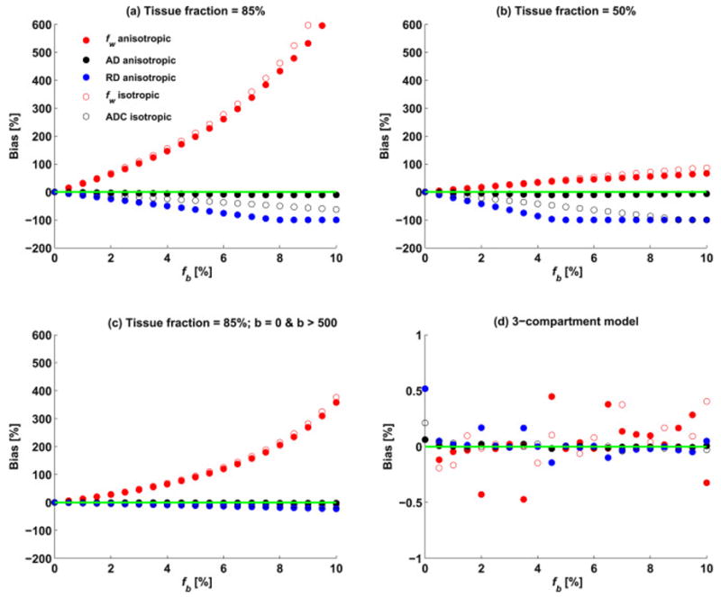
(a) Bias in the free water fraction (fw) and diffusion coefficients (AD and RD) as a function of the simulated blood fraction (fb) for the two-compartment model with the tissue fraction set to 85%. The bias in fw was much larger than the bias for AD and RD and increased as a function of fb. (b) Same simulation as in (a) with the tissue fraction set to 50% to represent a voxel with large CSF partial volume, showing that the bias in this case is reduced. (c) The same simulation as in (a) excluding low b-values, except for the b=0. While the bias is reduced it is still substantial for the estimation of fw, suggesting that the effects of perfusion are introduced by the b=0 image. (d) Same simulation as in (a) fitted using the three-compartment model. As expected, the bias in all model parameters was negligible.
Figure 1b shows the estimation of the two-compartment model parameters when the tissue fraction is set to 50%. Similar to Figure 1a, fw is over-estimated, and AD, and RD are underestimated. However, now the bias level of the fw parameter is lower and comparable to that of RD, and the bias in AD and RD is higher.
The simulation is repeated again in Figure 1c, for a tissue fraction of 85% and b-values that include b=0 and b>500 while excluding all other low b-values. We see that despite not including the lower b-values, except for b=0, the overestimation in fw is still very large, although not as large as when the lower b-values are included (compare with Figure. 1a).
The estimation bias in the diffusivities using the proposed three-compartment model is presented in Figure 1d. As would be expected for this noise-free simulation, the bias in all measures is negligible and is independent of fb.
Figure 2 shows the effect of perfusion on the estimation of free-water in the experiment that varied the minimal b-value. In this figure, the mean (Figure. 2a) and standard deviation (Figure. 2b) of the estimated fw are plotted as a function of the minimal b-value (bmin). As bmin increases, the mean estimated fw from the two-compartment model decreases towards the ground truth, reaching a minima around b=350 s/mm2. As bmin further increases, the mean estimated fw increases away from the ground truth. The standard deviation steadily increases as bmin increases. The figure also plots the mean estimated fw using the three-compartment model, showing that as bmin increases, the fit becomes less stable, i.e., the standard deviation steadily increases and the mean is shifted from the ground truth.
Figure 2.
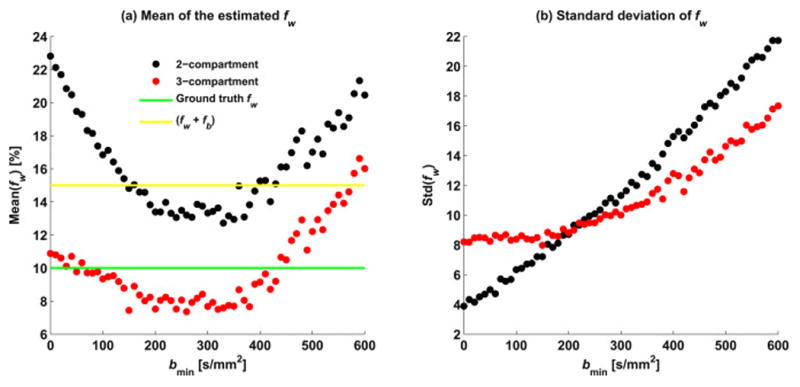
The two- and three-compartment fit estimations of the free water fraction as a function of the minimal b-value used. Plotted are the mean values of fw (a), and the standard deviation (b) for both models. Minimal b-value between b=200 and 350 s/mm2 reduces the perfusion effects, placing the estimated fw value between the 10% fw ground truth (green line) and the 15% border for non-tissue fraction (fw+fb; yellow line). At the same time the standard deviation is increased as bmin increases. Increasing the minimal b-value for the three-compartment model reduces the stability and accuracy of the model fit.
The robustness of the three-compartment and two-compartment model fit is evaluated in Figure 3a for different noise levels. In these experiments, the ground truth signal fractions were set to: fb=5%, fw=10%, and tissue fraction=85%. The variability in the three-compartment fit (red) was larger than the variability of the two-compartment fit (black) for all SNR levels. However, the mean fw estimated with the three-compartment fit was much closer to the ground truth than the mean fw estimated with the two-compartment fit.
Figure 3.
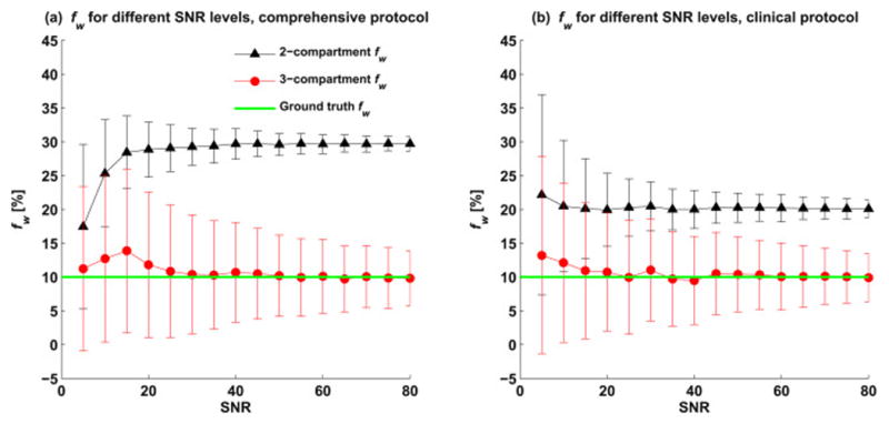
The effect of acquisition noise on the model fit. Estimated fw for different SNR levels, using both two- and three-compartment models are presented for (a) the comprehensive dataset protocol (44 b-values) and (b) the clinical protocol (b=0, 50, 200, 500, 900 and 1400 s/mm2). The error bars represent one standard deviation. The standard deviation for the clinical acquisition was higher than that of the comprehensive protocol. For both protocols, the two-compartment fit overestimated fw. However, in the clinical protocol, which included fewer low b-values, the bias was lower than that for the comprehensive protocol.
In Figure 3b further evaluations of the robustness of the two- and three-compartment fit, using the same b-shells and gradient scheme as in the clinical acquisition, are summarized. As expected, the variability in the estimation of fw increases compared to the multiple b-value acquisition simulated in Figure 3a. However, the mean fw estimated with the three-compartment model remained close to the true value. Note that the three-compartment fw estimate for the clinical data was closer to the ground truth than the two-compartment model.
3.2 In Vivo Human Data
Figure 4 shows the fb maps for the two acquisitions. The maps show that non-zero fb values are expected throughout the brain, with most values in the range between 0 and 20%. The histograms of the two acquisitions show a similar distribution of low fb values (fb<4%) with 55% of the voxels in the comprehensive acquisition and 53% of the voxels in the clinical acquisition falling in this range. The distribution for the comprehensive acquisition showed a higher percentage of intermediate values (4%<fb<10%), i.e., 30% of the voxels compared to 21% of the voxels in the clinical acquisition, and lower percentage of high fb values (fb>10%) with 15% of the voxels compared to 26% of the voxels in the clinical acquisition. The spatial distribution shows that in the comprehensive protocol high fb values were mainly at the border of the ventricles and around the brain parenchyma. In the clinical protocol, the lower resolution resulted in high fb values in the entire ventricles and with more hyperintense fb clusters in brain areas, probably due to noise effects and since the brain folding is no longer distinguishable at this resolution.
Figure 4.
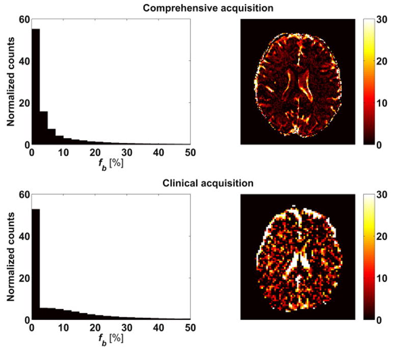
Histogram of the fb distribution over the whole brain and maps of a representative slice. The right column shows an example slice, which allows evaluating the spatial distribution. The left column shows a histogram of fb values across the whole brain (background excluded), which allows evaluating the accumulated fb distribution. The values from a comprehensive acquisition (upper row) and a clinical feasible acquisition (lower row) with fewer b-values are compared. A non-zero contribution of the blood component is seen across the brain, including both white and gray matter regions. A high signal fraction of blood was found in the ventricles and around the brain parenchyma.
Figure 5 demonstrates the differences between the two- and three-compartment fitted fw and diffusivities. Estimating fw using the two-compartment model yielded higher values than the three-compartment model, with both models providing high fw values in the CSF filled ventricles and CSF around the brain parenchyma. The difference between the fw maps (Figure 5c) shows that the three-compartment model had the most effect in these CSF filled voxels.
Figure 5.
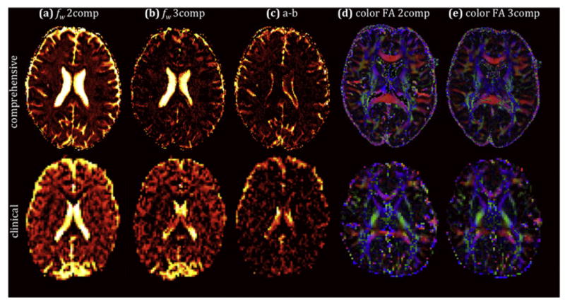
Free-water fraction (fw) maps obtained with both a two-compartment model (a) and a three-compartment model (b), and the corresponding difference map (c), showing overestimation of fw for the two-compartment model, when the blood compartment is ignored. Direction encoded color maps weighted by FA obtained with both the two-compartment model (d) and the three-compartment model (e) display comparable FA and directionality between the models. The bottom row shows the corresponding maps obtained with the clinically feasible protocol.
Similar to the fb map, it was harder to distinguish the brain/CSF interface in the clinical protocol with lower resolution. Figures 5d-e show very similar color by orientation FA maps between the two models.
Table 1 further characterizes the distribution of the fb and fw values in white matter. For the comprehensive protocol, the fb values in the white matter ROIs were in the range of 1.1% to 22.8%. However, values higher than 10% were found only in 3 of the regions (Fornix, and right and left superior cerebellar peduncle). The average fb across all white matter ROIs was 2.3%. For the clinical dataset, the fb values were in the range of 2.1% to 22.3%, with 6 ROIs that had values higher than 10% (Fornix, right and left superior cerebellar peduncle, right and left inferior cerebellar peduncle, and corticospinal tract on the right). These regions were bordering the ventricles. Fitting the three-compartment model instead of the two-compartment model decreased the mean fw over all white matter labels from 12.8% to 6.8% (46.9% decrease) in the comprehensive protocol, and from 16.8% to 11.3% (32.6% decrease) in the clinical protocol. In this table, the free water fraction, fw, is color-coded from bright to dark according to these ranges: 0-10% (yellow), 10-20% (orange), >20% (red). The percent change between the models is color coded from light blue (0-10%) to darker blue (10-20%), and the darkest blue (>20%).
Table 1.
Average fw and fb over white matter regions of interest using the two- and three-compartment models, with the comprehensive (left columns) and clinical (right columns) data sets. The free water fraction, fw, is color-coded from bright to dark according to these ranges: 0-10% (yellow), 10-20% (orange), >20% (red). The use of the three-compartment model decreased the fw value in most ROIs to the expected range of 0-10% for the comprehensive data. Similarly, for the clinical data there is a reduction in fw following the three-compartment model. The percent change between the models is color coded from light blue (0-10%) to darker blue (10-20%), and the darkest blue (>20%).
| Table 1 | fw 2comp [%] | fw 3comp [%] | 2comp vs. 3comp [% change] | fb 3comp [%] | fw 2comp [%] | fw 3comp [%] | 2comp vs. 3comp [% change] | fb 3comp [%] |
|---|---|---|---|---|---|---|---|---|
| WM regions | Comprehensive | Clinical | ||||||
| Pontine crossing tract (a part of MCP) | 20.6 | 4.3 | 79.2 | 7.1 | 18.6 | 13.0 | 30.2 | 4.7 |
| Genu of corpus callosum | 20.4 | 14.3 | 29.8 | 2.5 | 13.8 | 9.9 | 28.6 | 4.5 |
| Body of corpus callosum | 15.0 | 9.1 | 39.6 | 2.5 | 16.2 | 11.2 | 31.1 | 5.0 |
| Splenium of corpus callosum | 9.1 | 4.5 | 49.9 | 2.0 | 15.2 | 9.6 | 36.8 | 5.8 |
| Fornix (column and body of fornix) | 54.4 | 10.4 | 80.8 | 22.8 | 39.4 | 15.6 | 60.5 | 21.1 |
| Corticospinal tract R | 18.3 | 4.2 | 77.0 | 7.8 | 27.4 | 9.4 | 65.8 | 17.5 |
| Medial lemniscus R | 8.4 | 2.5 | 69.8 | 2.6 | 14.3 | 11.2 | 21.9 | 2.6 |
| Medial lemniscus L | 11.3 | 3.5 | 69.1 | 3.4 | 15.0 | 11.7 | 22.1 | 2.5 |
| Inferior cerebellar peduncle R | 17.5 | 6.0 | 65.6 | 5.6 | 29.3 | 9.4 | 67.8 | 18.5 |
| Inferior cerebellar peduncle L | 16.1 | 4.9 | 69.3 | 6.2 | 30.4 | 13.9 | 54.2 | 14.4 |
| Superior cerebellar peduncle R | 22.2 | 5.0 | 77.5 | 10.0 | 33.5 | 14.0 | 58.1 | 17.0 |
| Superior cerebellar peduncle L | 25.2 | 4.5 | 82.1 | 11.6 | 40.0 | 13.5 | 66.3 | 22.3 |
| Cerebral peduncle R | 12.4 | 4.1 | 67.2 | 3.4 | 15.2 | 8.0 | 47.4 | 7.7 |
| Cerebral peduncle L | 10.8 | 5.5 | 49.1 | 2.3 | 14.1 | 7.9 | 44.1 | 5.9 |
| Anterior limb of internal capsule R | 10.9 | 4.2 | 61.0 | 2.6 | 17.3 | 12.1 | 30.0 | 4.7 |
| Anterior limb of internal capsule L | 10.3 | 4.9 | 52.5 | 2.1 | 12.9 | 7.8 | 39.4 | 5.0 |
| Posterior limb of internal capsule R | 9.8 | 4.1 | 58.0 | 2.1 | 14.6 | 10.3 | 30.0 | 3.8 |
| Posterior limb of internal capsule L | 10.7 | 5.7 | 46.8 | 1.8 | 12.2 | 7.9 | 35.6 | 3.8 |
| Retrolenticular part of internal capsule R | 9.6 | 4.0 | 58.6 | 2.0 | 15.8 | 11.2 | 29.2 | 4.0 |
| Retrolenticular part of internal capsule L | 11.7 | 6.7 | 42.6 | 1.7 | 14.7 | 10.4 | 29.1 | 3.6 |
| Anterior corona radiata R | 12.7 | 5.8 | 53.8 | 2.3 | 16.7 | 12.4 | 25.6 | 3.6 |
| Anterior corona radiata L | 11.3 | 6.5 | 42.4 | 1.6 | 17.7 | 12.5 | 29.4 | 4.3 |
| Superior corona radiata R | 10.4 | 5.5 | 47.5 | 1.7 | 17.1 | 11.8 | 31.1 | 4.4 |
| Superior corona radiata L | 11.6 | 6.6 | 43.0 | 1.7 | 15.9 | 12.5 | 21.0 | 2.7 |
| Posterior corona radiata R | 11.4 | 6.7 | 41.2 | 1.6 | 17.2 | 12.9 | 24.9 | 3.6 |
| Posterior corona radiata L | 12.6 | 7.0 | 44.6 | 1.9 | 17.3 | 13.6 | 21.6 | 3.0 |
| Posterior thalamic radiation R | 11.2 | 6.1 | 45.5 | 1.8 | 13.9 | 9.6 | 30.8 | 3.6 |
| Posterior thalamic radiation L | 13.7 | 8.2 | 40.4 | 1.8 | 16.2 | 11.7 | 27.4 | 3.5 |
| Sagittal stratum (include ILF and IFOF) R | 14.3 | 7.0 | 50.9 | 2.4 | 18.8 | 12.4 | 33.8 | 4.9 |
| Sagittal stratum (include ILF and IFOF) L | 16.7 | 6.9 | 59.0 | 3.4 | 15.8 | 11.1 | 29.6 | 3.6 |
| External capsule R | 7.2 | 3.7 | 48.8 | 1.3 | 17.8 | 13.1 | 26.7 | 3.9 |
| External capsule L | 8.1 | 5.2 | 36.4 | 1.1 | 17.3 | 11.4 | 34.1 | 4.8 |
| Cingulum (cingulate gyrus) R | 9.5 | 5.8 | 38.8 | 1.4 | 17.5 | 13.7 | 21.8 | 4.1 |
| Cingulum (cingulate gyrus) L | 10.0 | 6.2 | 37.9 | 1.5 | 19.6 | 14.7 | 25.1 | 5.0 |
| Cingulum (hippocampus) R | 15.0 | 5.1 | 66.2 | 3.8 | 18.6 | 11.1 | 40.5 | 5.8 |
| Cingulum (hippocampus) L | 17.5 | 4.1 | 76.3 | 5.8 | 17.5 | 9.5 | 45.6 | 6.8 |
| Fornix (cres) / Stria terminalis R | 20.7 | 9.5 | 53.9 | 3.8 | 23.5 | 14.9 | 36.6 | 7.2 |
| Fornix (cres) / Stria terminalis L | 17.1 | 8.6 | 50.0 | 3.0 | 16.9 | 10.8 | 35.7 | 4.9 |
| Superior longitudinal fasciculus R | 10.5 | 5.8 | 44.5 | 1.5 | 13.7 | 9.7 | 28.8 | 3.6 |
| Superior longitudinal fasciculus L | 11.3 | 7.7 | 32.1 | 1.2 | 16.2 | 12.3 | 23.9 | 3.2 |
| Superior fronto-occipital fasciculus R | 11.9 | 5.6 | 53.0 | 2.2 | 22.9 | 14.9 | 34.9 | 6.8 |
| Superior fronto-occipital fasciculus L | 11.2 | 6.1 | 45.1 | 1.7 | 18.2 | 11.7 | 36.0 | 5.9 |
| Uncinate fasciculus R | 6.1 | 2.8 | 54.3 | 1.2 | 19.6 | 15.6 | 20.3 | 3.2 |
| Uncinate fasciculus L | 4.9 | 2.1 | 57.8 | 1.1 | 12.8 | 10.1 | 20.6 | 2.1 |
| Tapetum R | 44.0 | 36.9 | 16.3 | 3.2 | 30.5 | 17.0 | 44.3 | 8.6 |
| Tapetum L | 58.2 | 44.4 | 23.8 | 7.6 | 32.5 | 21.8 | 32.8 | 6.5 |
| ALL WHITE MATTER LABELS | 12.8 | 6.8 | 46.9 | 2.4 | 16.8 | 11.3 | 32.6 | 4.9 |
Additional characterization of differences in diffusivity measures (FA, MD, AD and RD) is provided in Supplementary Tables 1-2. Comparing the FA in the white matter ROIs of both acquisitions indicate that differences in FA were most prominent between the one- and two-compartment models (on average a 20.7% decrease in FA), and less prominent when comparing the two- and three-compartment models (on average a 2.2% increase in FA). Similar to FA, changes in MD, AD and RD were most pronounced between the one- and two-compartment models, and less so between the two- and three-compartment models (see Supplementary Tables 1-2). The largest difference between the two- and three-compartment models was the overestimation of fw.
Figure 6 shows bias ((2comp-3comp)/3comp) as a function of the fb, for FA (left) and fw (right) in all white matter regions for both acquisition types, revealing an order of magnitude higher bias in fw compared to the bias in FA.
Figure 6.
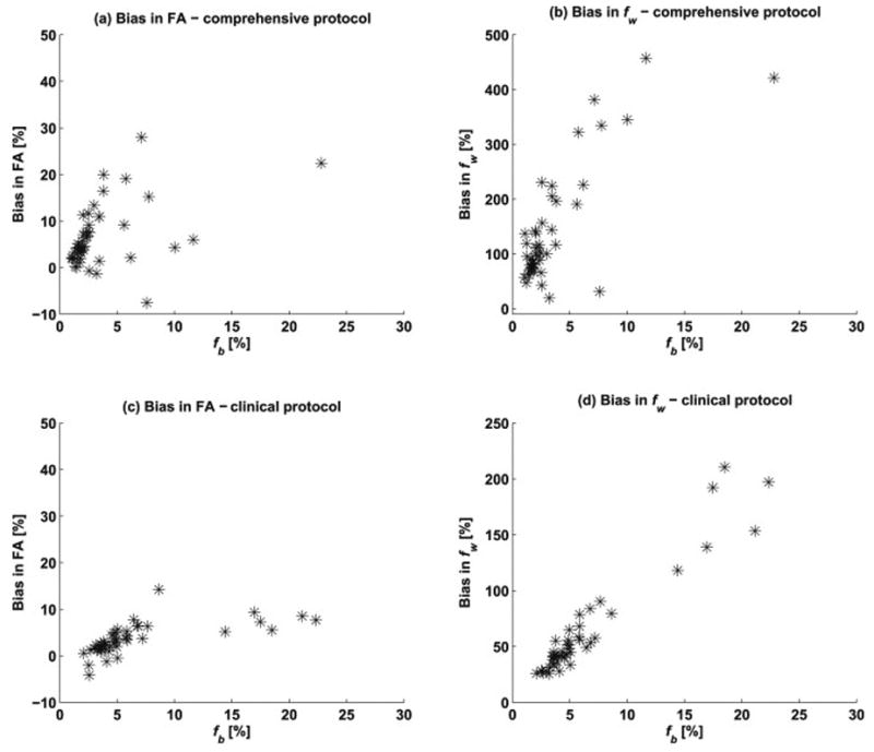
Bias in the two-compartment parameter fit (compared with the three-compartment values) of (a) FA and (b) fw, as a function of fb, in all white matter regions for the comprehensive acquisition. There was higher bias in fw compared to the bias in FA. Notice that the scale for the fw bias is 20 times larger than that of the FA bias. Figures (c) and (d) show a similar pattern for the bias in fw and fb, respectively, in the dataset acquired with the clinical protocol.
4 Discussion
The present study demonstrates that blood flow in the capillary bed may have a dramatic effect on the estimation of the free water fraction from a two-compartment model that does not explicitly account for perfusion effects. The results indicate that a three-compartment model is a feasible approach for correcting for the perfusion effect, as well as for quantifying the signal fraction of the blood compartment, which is indicative of capillary blood volume. A small, yet consistent contribution from the capillary blood compartment was observed in in vivo human brain scans. If the capillary blood compartment is not included in the model, the fw parameter is considerably overestimated, even for small perfusion contributions. The perfusion effect was less pronounced in the estimations of tensor diffusivities, suggesting that the fast IVIM contribution of perfusion is mainly captured by the free water compartment. Importantly, our results show that the perfusion effects remain even when low b-values are removed and only a single b=0 is included in the fit.
The fact that perfusion affects the estimation of diffusivities is well established (27). However, the present study challenges the common misconception that perfusion does not affect DTI-like acquisitions when low b-value shells are not collected. The results in Figure 1c confirm that the exclusion of low b-values reduces the perfusion effect. However, they also demonstrate that the effect is maintained as long as a b=0 volume (or another low b-value volume) is included in the analysis (27). Most acqusition protocols include at least one low b-value volume, usually as a baseline reference, which means that the perfusion effects we report here are relevant to most protocols that are used.
In a DTI model, perfusion appears as fast pseudo diffusion, increasing the estimates of the diffusivities. However, the results suggest that when another fast diffusing compartment is included in the model, i.e., a free-water compartment, this fast diffusing compartment will absorb most of the perfusion effects (see, e.g., Figure 1), resulting in an overestimation of the fw parameter. The other diffusivity parameters are then less affected by the pefusion (slight underestimation). This finding supports recent studies proposing that free-water corrected diffusivities are capable of correcting for most extracellular effects, including those of perfusion, and are therefore more specific to tissue than non-corrected DTI parameters (4, 44). On the other hand, the observed overestimation of the fw parameter suggests that changes in the arrangment of the capillaries or the properties of the perfused blood may have contributed to some of the previous observations attributed to increased fw in the literature (4, 13, 14). Some two-compartment free-water imaging studies are focused on the tissue fraction (11, 12), which is mathematically equal to 1-fw. Therefore, whenever fw is overestimated, the tissue fraction will be underestimated, although usually not to the same extent as the bias in the fw parameter. For example, consider a case where the true free-water fraction is 10%, the true blood fraction is 5%, and the true tissue fraction is 85%. Our simulations show that the two-compartment model will overestimate the fw parameter by about 200%, yielding fw of about 20%. The tissue fraction would then be 80% which is about 6% under-estimation from the true 85% fraction. Such vascular effects could potentially be identified and separated from extracellular diffusion effects using the proposed three-compartment model.
Two approaches to reduce the perfusion effect were explored in this study: (i) increasing the minimal b-value used in the fitting, and (ii) using a three-compartment model that explicitly accounts for a blood compartment. By increasing the minimal b-value used in the fitting, the contribution of perfusion was decreased and thus the bias was reduced as well (see Figure 2). However, eliminating the bias requires relatively high minimal b-value. The contrast between the high and low b-values is then decimated, which increases the standard deviation of the fit, i.e., reduces the stability of the fit. We find that a minimal b-value in the range of 200-350 s/mm2 effectively eliminates the perfusion effect, with the cost of higher standard deviation. As the minimal b-value increases further, the model fit becomes less stable with increased standard deviation and reduced accuracy, likely since in the higher b-values the signal from the free-water compartment is attenuated as well, making it impossible to estimate.
As could be expected, our simulations demonstrated that the quality of the three-compartment fit improves when low b-values are included. This is because the low b-value volumes include perfusion signal that is no longer there in the higher b-values. The standard deviation of the estimates obtained by the three-compartment model (see Figure 3) was larger than that of the two-compartment fit, suggesting that the additional parameter makes the fit less stable. At the same time, the three-compartment model resulted in a more correct mean fw, suggesting that noise removal approaches, or more robust fitting approaches, are more likely to result in both a stable and non-biased estimation of fw. Even though the analyses in this study were performed using the two-compartment free-water model, a very similar bias in the estimation of fw is to be expected in any other model that includes a free-water compartment in addition to other compartments that model the slower diffusing components.
The extent of the perfusion effects was demonstrated by the in vivo human data, for which the observed levels of fb with the comprehensive acquisition were between 1% and 3% in most (30 of 43) white matter ROIs, which is in accordance with previous studies (32, 45). However, as predicted by the simulations, even though fb had low values, the effect on the estimation of fw was considerable. Here, we only evaluated white matter regions, however, in future studies gray matter regions can also be considered, in which case special care has to be taken with regards to ROI placement in the diffusion space, in order to avoid registration errors and partial volume with CSF. Higher fb values were found mainly in the ventricles and around the brain parenchyma, suggesting that our model may not provide optimal fits in pure CSF voxels (see e.g., Figure 5c). Nevertheless, the simulations predict that the perfusion effects are less pronounced in voxels with a significant partial volume of CSF (see Figure 1b).
Accounting for perfusion with the three-compartment model reduced fw to values below 10% in many regions, which is in better agreement with the expected extracellular volume (46). This reduction in fw was especially prominent in the fornix, which is known to show overestimated fw values (and underestimated FA) with the two-compartment model (47). Of note, the fornix provided higher than expected fb values, which might be explained by subject motion, pulsation, poor registration or flow artifacts in the vicinity of the ventricles, captured by fb. However, the increased fb could also reflect partial volume with blood within the capillaries of the choroid plexus and the capillaries that line the ventricles (48), which would have higher volume than capillaries in white matter. These effects may explain the fb values in CSF that appear to be higher than in tissue. While more studies are required to understand fb values in CSF, applications that are more interested in brain tissue may choose to discard voxels with apparent diffusivity that is faster than free-water from the model fit. Better validation methods, for example, animal models where capillary blood volume can be manipulated, are required to understand the contribution of fb in different parts of the brain. Validation can also be achieved by comparing fb with CBV measures obtained, for example, by DSC- or DCE-MRI. Interestingly, the largest changes in FA and other tensor based measures occurred when shifting from the one-compartment to the two-compartment model. Between the two-compartment and the three-compartment model the change was limited, suggesting that tensor based measures are contaminated by a fast component of random motion, which the two-compartment model, as stated above, is capable of resolving reasonably well.
A number of limitations of the three-compartment model should also be noted. The fractional signals should not be considered as physical quantities, but rather as a comparative quantity. In our model, the diffusivity of the blood compartment was set to an approximate value, unlike the diffusivity of free-water, which is well defined (depending on temperature and viscosity). The effective diffusivity of the blood compartment, Df, may change in time and space (18, 20). Changes in the Df will, in turn, affect the estimation of fb, which means that care should be taken with the interpretation of fb as an unbiased physical measure. Simulations, however, demonstrated that the choice of Df had little effect on the estimation of fw and diffusivities (see Supplementary Figure 1). This suggests that as long as a faster compartment is included, the slower compartments will be accurately estimated. It also suggests that any signal that may appear as fast diffusing, e.g., subject motion, Gibbs artifacts, mis-registration etc., is more likely to be modeled by the fast diffusing compartment, affecting the estimation of fb. Therefore data preprocessing is essential, especially for the estimation of fb. In future models, one might consider adding Df as a free parameter as well, which may further disentangle different sources of changes in the blood compartment. While we focused on the effects of perfusion on the estimation of free-water and other diffusivities in this work, the fact that free-water is a fast diffusing compartment suggests that not including a free-water compartment, as in the original IVIM model (Eq. 3) for example, will bias the fb estimation. A three-compartment model may thus provide more reliable fb estimations than a two-compartment IVIM model, although this hypothesis is not directly tested here.
The models studied in this paper are compartmental models, with the inherent limitation of including a finite number of compartments. Previous studies have suggested that biological tissue might be composed of a large number of apparent diffusion compartments that do not necessarily represent biological compartments (49). It has been argued that biological compartments may be better described by variability or heterogeneity measures (49-51), as well as by time dependent diffusion (49, 52). In our model, the tensor representing the tissue compartment is further simplified by assuming cylindrical symmetry, which may be a good approximation for single white matter bundles, but might not be accurate for certain configurations of complex fiber architecture, where single tensors may not be a good approximation anyways. The cylindrical symmetry approximation reduced the number of parameters, and provided a simple approach for preventing negative eigenvalues. Alternative ways to represent the tissue may be considered in future work. We note that unlike the tissue compartment, the free-water compartment is appropriately modeled by an isotropic diffusion tensor, and therefore accurate approximation of this compartment and elimination of its signal could be a useful initial step towards more complicated diffusion models. The blood compartment in our model is limited to a single isotropic compartment, while it could be the case that the contribution of capillary blood is orientation dependent, as was identified in myocardial tissue (53, 54), in muscles (55, 56), and suggested for the brain (56). Future studies may consider a more elaborate representation of Df, which may account for perfusion anisotropy.
Comparing the comprehensive data acquisition with the more clinically feasible acquisition shows that as the number of low b-values is decreased, there is higher risk of over-estimating fb, which is in agreement with previous studies showing that lower SNR results in overestimation of fb from the IVIM mode (57). Moreover, the fractional volume parameters are weighted by the T1 and T2 relaxation times, which are not accounted for in the current model. Previous studies have shown that relaxation compensation could be included in the IVIM model (32, 58, 59) to get a better estimation of the fractional volumes and to separate the different components. However, this will significantly increase the acquisition time, as well as the number of model parameters. Nevertheless, as long as the acquisition parameters are identical across a cohort of subjects, the signal fractions can be considered for direct comparison between groups.
Further numerical simulations and test-retest analyses are required to define an optimal acquisition for the three-compartment model. As is the case for all imaging sequences, the selection of an optimal acquisition will be a trade-off between acquisition time, SNR, and the effect size expected (60). A clinical protocol also has to take into account whether additional diffusion MRI information is desired. For example, to disentangle complex fiber architecture a larger number of gradient orientations may be preferred, as well as possibly additional higher b-values. In more typical clinical acquisitions that do not include low b-shells, multiple acquisitions of a b=0 image would further increase the precision of the model fit (61). However, as long as one or more b=0 are included, perfusion will still bias any estimated diffusivities (see Figure 1c). The clinical sequence that we proposed here could be further improved if running on a 3T or 7T magnet by opting for higher resolution, preferably with isotropic voxels, since in our experiments resolution appears to affect the fb and fw estimates. Higher resolution could likely also improve the quality of the registration. Additional improvements, such as multi-band acquisition may be considered to significantly shorten the scan time of a clinical protocol, or alternatively could allow the addition of more b-value shells.
In our experiments the protocols were tested on two different subjects, and it is very likely that the model parameters vary between subjects, especially with age (6). Better characterization of the model parameters is needed in a larger cohort of subjects, to study age and gender effects, as well as other possible contributors.
Future studies should also consider comparing the proposed method with modified sequence approaches for improved estimation or elimination of perfusion effects in IVIM imaging. For example, magnetization preparation such as inversion (62) or T2-preparation (63) could be used to better separate the different compartments. Furthermore, by using double diffusion encodings, the IVIM estimation can be improved by varying the flow compensation and comparing anti-parallel acquisitions (45). Finally, efficient gradient waveforms for isotropic weighting (64) can be used to remove the effects of diffusion anisotropy (65, 66). Since in our model the perfusion and the free-water are both isotropic, acquisitions that rely on isotropic weighting may prove to be more appropriate for the model estimation.
5 Conclusions
The results indicate that a three-compartment model that includes an additional compartment to model perfusion improves the estimation of the free water fraction. Such a model disentangles the perfusion effect from that of free water, and with adequate acquisition, as well as model fitting approaches, it could distinguish between changes that originate from capillary blood perfusion versus those that originate from diffusion in the extracellular space. Separating these effects in future clinical studies would allow for a more specific characterization of heterogeneous tissues, which is especially important in disorders involving a combination of vascular, edematous, and tissue changes such as Alzheimer's disease, vascular dementia, and brain injuries. Interpretation of results from two-compartment analysis should be taken with care since fw estimates may be affected by both water and blood.
Supplementary Material
Supplementary Table 1 a-b. JHU-atlas of white matter regions, registered to parametric maps obtained with one-, two-, and three-compartment models, for the comprehensive protocol. Table 1a shows FA and MD, and Table 1b shows RD and AD. % change is color coded from light blue (0-10%) to darker blue (10-20%), and the darkest blue (>20%).
Supplementary Table 2 a-b. JHU-atlas of white matter regions, registered to parametric maps, for the dataset obtained with the clinically feasible protocol using fewer b-shells. Table 2a shows FA and MD, and Table 2b shows RD and AD. The color-coding is the same as in Table 1 (a-b).
Supplementary Figure 1. Bias in fw for different numbers of gradient directions – 6 directions (a), 12 directions (b) and 30 directions (c). The second row shows the effect of changing Df , using 25 μm2/ms (e) 50 μm2/ms (f) and 100 μm2/ms, which can be compared to plot (a) which shows the bias for a Df of 10 μm2/ms.
Highlights.
Perfusing capillary blood affects the estimation of diffusivities.
Other fast diffusing components such as the free water fraction are overestimated.
A three-compartment model including tissue, free water and blood is proposed.
Separating perfusing blood signal from water diffusion improves freewater estimation.
Clinical feasibility is demonstrated with simulations and real data.
Acknowledgments
Thanks to Sophia Swago, who provided language edits.
Funding: This work was supported by NIH grants [grant numbers R01MH108574, R01MH074794, P41EB015902, R01AG042512, R01MH102377]; the Swedish Foundation for Strategic Research (SSF) [grant number AM13-0090]; and the Swedish Research Council [grant number 13514].
Abbreviations
- IVIM
intravoxel incoherent motion
- ADC
apparent diffusion coefficient
- CSF
cerebrospinal fluid
- DTI
diffusion tensor imaging
- FA
fractional anisotropy
- RD
radial diffusivity
- AD
axial diffusivity
- SNR
signal-to-noise ratio
- MD
mean diffusivity
- ROI
region of interest
Footnotes
Publisher's Disclaimer: This is a PDF file of an unedited manuscript that has been accepted for publication. As a service to our customers we are providing this early version of the manuscript. The manuscript will undergo copyediting, typesetting, and review of the resulting proof before it is published in its final citable form. Please note that during the production process errors may be discovered which could affect the content, and all legal disclaimers that apply to the journal pertain.
References
- 1.Le Bihan D. Looking into the functional architecture of the brain with diffusion MRI. Nat Rev Neurosci. 2003;4(6):469–80. doi: 10.1038/nrn1119. [DOI] [PubMed] [Google Scholar]
- 2.Mills R. Self-diffusion in normal and heavy water in the range 1-45.deg. The Journal of Physical Chemistry. 1973;77(5):685–8. [Google Scholar]
- 3.Holz M, Heil SR, Sacco A. Temperature-dependent self-diffusion coefficients of water and six selected molecular liquids for calibration in accurate 1H NMR PFG measurements. Physical Chemistry Chemical Physics. 2000;2(20):4740–2. [Google Scholar]
- 4.Pasternak O, Westin CF, Bouix S, Seidman LJ, Goldstein JM, Woo TUW, et al. Excessive Extracellular Volume Reveals a Neurodegenerative Pattern in Schizophrenia Onset. The Journal of Neuroscience. 2012;32(48):17365–72. doi: 10.1523/JNEUROSCI.2904-12.2012. [DOI] [PMC free article] [PubMed] [Google Scholar]
- 5.Pasternak O, Sochen N, Gur Y, Intrator N, Assaf Y. Free water elimination and mapping from diffusion MRI. Magnetic Resonance in Medicine. 2009;62(3):717–30. doi: 10.1002/mrm.22055. [DOI] [PubMed] [Google Scholar]
- 6.Metzler-Baddeley C, O'Sullivan MJ, Bells S, Pasternak O, Jones DK. How and how not to correct for CSF-contamination in diffusion MRI. NeuroImage. 2012;59(2):1394–403. doi: 10.1016/j.neuroimage.2011.08.043. [DOI] [PubMed] [Google Scholar]
- 7.Zhang H, Schneider T, Wheeler-Kingshott CA, Alexander DC. NODDI: Practical in vivo neurite orientation dispersion and density imaging of the human brain. NeuroImage. 2012;61(4):1000–16. doi: 10.1016/j.neuroimage.2012.03.072. [DOI] [PubMed] [Google Scholar]
- 8.Barazany D, Basser PJ, Assaf Y. In vivo measurement of axon diameter distribution in the corpus callosum of rat brain. Brain. 2009;132(5):1210–20. doi: 10.1093/brain/awp042. [DOI] [PMC free article] [PubMed] [Google Scholar]
- 9.Wang Y, Wang Q, Haldar JP, Yeh FC, Xie M, Sun P, et al. Quantification of increased cellularity during inflammatory demyelination. Brain. 2011;134(12):3587–98. doi: 10.1093/brain/awr307. [DOI] [PMC free article] [PubMed] [Google Scholar]
- 10.Pasternak O, Kubicki M, Shenton ME. In vivo imaging of neuroinflammation in schizophrenia. Schizophrenia research. 2016;173(3):200–12. doi: 10.1016/j.schres.2015.05.034. [DOI] [PMC free article] [PubMed] [Google Scholar]
- 11.Berlot R, Metzler-Baddeley C, Jones DK, O'Sullivan MJ. CSF contamination contributes to apparent microstructural alterations in mild cognitive impairment. Neuroimage. 2014;92:27–35. doi: 10.1016/j.neuroimage.2014.01.031. [DOI] [PMC free article] [PubMed] [Google Scholar]
- 12.Metzler-Baddeley C, Hunt S, Jones DK, Leemans A, Aggleton JP, O'Sullivan MJ. Temporal association tracts and the breakdown of episodic memory in mild cognitive impairment. Neurology. 2012;79(23):2233–40. doi: 10.1212/WNL.0b013e31827689e8. [DOI] [PMC free article] [PubMed] [Google Scholar]
- 13.Maier-Hein KH, Westin CF, Shenton ME, Weiner MW, Raj A, Thomann P, et al. Widespread white matter degeneration preceding the onset of dementia. Alzheimer's & dementia : the journal of the Alzheimer's Association. 2015;11(5):485–93.e2. doi: 10.1016/j.jalz.2014.04.518. [DOI] [PMC free article] [PubMed] [Google Scholar]
- 14.Ofori E, Pasternak O, Planetta PJ, Li H, Burciu RG, Snyder AF, et al. Longitudinal changes in free-water within the substantia nigra of Parkinson's disease. Brain. 2015;138(8):2322–31. doi: 10.1093/brain/awv136. [DOI] [PMC free article] [PubMed] [Google Scholar]
- 15.Pasternak O, Koerte IK, Bouix S, Fredman E, Sasaki T, Mayinger M, et al. Hockey Concussion Education Project, Part 2. Microstructural white matter alterations in acutely concussed ice hockey players: a longitudinal free-water MRI study. Journal of neurosurgery. 2014;120(4):873–81. doi: 10.3171/2013.12.JNS132090. [DOI] [PMC free article] [PubMed] [Google Scholar]
- 16.Le Bihan D, Breton E, Lallemand D, Grenier P, Cabanis E, Laval-Jeantet M. MR imaging of intravoxel incoherent motions: application to diffusion and perfusion in neurologic disorders. Radiology. 1986;161(2):401–7. doi: 10.1148/radiology.161.2.3763909. [DOI] [PubMed] [Google Scholar]
- 17.Bihan DL, Breton E, Lallemand D, Aubin ML, Vignaud J, Laval-Jeantet M. Separation of diffusion and perfusion in intravoxel incoherent motion MR imaging. Radiology. 1988;168(2):497–505. doi: 10.1148/radiology.168.2.3393671. [DOI] [PubMed] [Google Scholar]
- 18.Wirestam R, Borg M, Brockstedt S, Lindgren A, Holtas S, Stahlberg F. Perfusion-related parameters in intravoxel incoherent motion MR imaging compared with CBV and CBF measured by dynamic susceptibility-contrast MR technique. Acta Radiol. 2001;42:123. [PubMed] [Google Scholar]
- 19.Federau C, Maeder P, O'Brien K, Browaeys P, Meuli R, Hagmann P. Quantitative Measurement of Brain Perfusion with Intravoxel Incoherent Motion MR Imaging. Radiology. 2012;265(3):874–81. doi: 10.1148/radiol.12120584. [DOI] [PubMed] [Google Scholar]
- 20.Federau C, O'Brien K, Meuli R, Hagmann P, Maeder P. Measuring brain perfusion with intravoxel incoherent motion (IVIM): initial clinical experience. Journal of Magnetic Resonance Imaging. 2014;39(3):624–32. doi: 10.1002/jmri.24195. [DOI] [PubMed] [Google Scholar]
- 21.Togao O, Hiwatashi A, Yamashita K, Kikuchi K, Mizoguchi M, Yoshimoto K, et al. Differentiation of high-grade and low-grade diffuse gliomas by intravoxel incoherent motion MR imaging. Neuro-Oncology. 2016;18(1):132–41. doi: 10.1093/neuonc/nov147. [DOI] [PMC free article] [PubMed] [Google Scholar]
- 22.Le Bihan D, Turner R. The capillary network: a link between IVIM and classical perfusion. Magn Reson Med. 1992;27:171. doi: 10.1002/mrm.1910270116. [DOI] [PubMed] [Google Scholar]
- 23.Rosen BR, Belliveau JW, Vevea JM, Brady TJ. Perfusion imaging with NMR contrast agents. Magnetic resonance in medicine. 1990;14(2):249–65. doi: 10.1002/mrm.1910140211. [DOI] [PubMed] [Google Scholar]
- 24.Dixon WT, Du LN, Faul DD, Gado M, Rossnick S. Projection angiograms of blood labeled by adiabatic fast passage. Magnetic Resonance in Medicine. 1986;3(3):454–62. doi: 10.1002/mrm.1910030311. [DOI] [PubMed] [Google Scholar]
- 25.Calamante F, Thomas DL, Pell GS, Wiersma J, Turner R. Measuring cerebral blood flow using magnetic resonance imaging techniques. Journal of cerebral blood flow & metabolism. 1999;19(7):701–35. doi: 10.1097/00004647-199907000-00001. [DOI] [PubMed] [Google Scholar]
- 26.Sourbron SP, Buckley DL. Classic models for dynamic contrast-enhanced MRI. NMR in Biomedicine. 2013;26(8):1004–27. doi: 10.1002/nbm.2940. [DOI] [PubMed] [Google Scholar]
- 27.Padhani AR, Liu G, Mu-Koh D, Chenevert TL, Thoeny HC, Takahara T, et al. Diffusion-Weighted Magnetic Resonance Imaging as a Cancer Biomarker: Consensus and Recommendations. Neoplasia. 2009;11(2):102–25. doi: 10.1593/neo.81328. [DOI] [PMC free article] [PubMed] [Google Scholar]
- 28.Basser PJ, Mattiello J, LeBihan D. MR diffusion tensor spectroscopy and imaging. Biophysical Journal. 1994;66(1):259–67. doi: 10.1016/S0006-3495(94)80775-1. [DOI] [PMC free article] [PubMed] [Google Scholar]
- 29.Pasternak O, Shenton ME, Westin CF. In: Ayache N, Delingette H, Golland P, Mori K, editors. Estimation of Extracellular Volume from Regularized Multishell Diffusion MRI; Medical Image Computing and Computer-Assisted Intervention – MICCAI 2012: 15th International Conference; Nice, France. October 1-5, 2012; Proceedings, Part II. Berlin, Heidelberg: Springer Berlin Heidelberg; 2012. pp. 305–12. [DOI] [PMC free article] [PubMed] [Google Scholar]
- 30.Hoy AR, Koay CG, Kecskemeti SR, Alexander AL. Optimization of a Free Water Elimination Two-Compartment Model for Diffusion Tensor Imaging. NeuroImage. 2014;103:323–33. doi: 10.1016/j.neuroimage.2014.09.053. [DOI] [PMC free article] [PubMed] [Google Scholar]
- 31.Stejskal EO, Tanner JE. Spin diffusion measurements: spin-echo in the presence of a time dependent field gradient. J Chem Phys. 1965;42:288. [Google Scholar]
- 32.Rydhög AS, van Osch MJ, Lindgren E, Nilsson M, Lätt J, Ståhlberg F, et al. Intravoxel incoherent motion (IVIM) imaging at different magnetic field strengths: What is feasible? Magnetic resonance imaging. 2014;32(10):1247–58. doi: 10.1016/j.mri.2014.07.013. [DOI] [PubMed] [Google Scholar]
- 33.Federau C, Meuli R, O'Brien K, Maeder P, Hagmann P. Perfusion Measurement in Brain Gliomas with Intravoxel Incoherent Motion MRI. American Journal of Neuroradiology. 2014;35(2):256–62. doi: 10.3174/ajnr.A3686. [DOI] [PMC free article] [PubMed] [Google Scholar]
- 34.Nicolas R, Sibon I, Hiba B. Accuracies and Contrasts of Models of the Diffusion-Weighted-Dependent Attenuation of the MRI Signal at Intermediate b-values. Magnetic resonance insights. 2015;8:11. doi: 10.4137/MRI.S25301. [DOI] [PMC free article] [PubMed] [Google Scholar]
- 35.Ohno N, Miyati T, Kobayashi S, Gabata T. Modified triexponential analysis of intravoxel incoherent motion for brain perfusion and diffusion. Journal of Magnetic Resonance Imaging. 2016;43(4):818–23. doi: 10.1002/jmri.25048. [DOI] [PubMed] [Google Scholar]
- 36.Pasternak O, Assaf Y, Intrator N, Sochen N. Variational multiple-tensor fitting of fiber-ambiguous diffusion-weighted magnetic resonance imaging voxels. Magnetic Resonance Imaging. 2008;26(8):1133–44. doi: 10.1016/j.mri.2008.01.006. [DOI] [PubMed] [Google Scholar]
- 37.Pekar J, Moonen CT, van Zijl PC. On the precision of diffusion/perfusion imaging by gradient sensitization. Magn Reson Med. 1992;23:122. doi: 10.1002/mrm.1910230113. [DOI] [PubMed] [Google Scholar]
- 38.Chang LC, Koay CG, Pierpaoli C, Basser PJ. Variance of estimated DTI-derived parameters via first-order perturbation methods. Magnetic Resonance in Medicine. 2007;57(1):141–9. doi: 10.1002/mrm.21111. [DOI] [PubMed] [Google Scholar]
- 39.Jones DK, Cercignani M. Twenty - five pitfalls in the analysis of diffusion MRI data. NMR in Biomedicine. 2010;23(7):803–20. doi: 10.1002/nbm.1543. [DOI] [PubMed] [Google Scholar]
- 40.Assaf Y, Freidlin RZ, Rohde GK, Basser PJ. New modeling and experimental framework to characterize hindered and restricted water diffusion in brain white matter. Magnetic Resonance in Medicine. 2004;52(5):965–78. doi: 10.1002/mrm.20274. [DOI] [PubMed] [Google Scholar]
- 41.Westin CF, Pasternak O, Knutsson H. Rotationally invariant gradient schemes for diffusion MRI. Proceedings of the 20th ISMRM meeting. 2012 [Google Scholar]
- 42.Klein S, Staring M, Murphy K, Viergever MA, Pluim JPW. elastix: A Toolbox for Intensity-Based Medical Image Registration. IEEE Transactions on Medical Imaging. 2010;29(1):196–205. doi: 10.1109/TMI.2009.2035616. [DOI] [PubMed] [Google Scholar]
- 43.Wakana S, Jiang H, Nagae-Poetscher LM, Zijl PCMv, Mori S. Fiber Tract–based Atlas of Human White Matter Anatomy. Radiology. 2004;230(1):77–87. doi: 10.1148/radiol.2301021640. [DOI] [PubMed] [Google Scholar]
- 44.Bergamino M, Pasternak O, Farmer M, Shenton ME, Paul Hamilton J. Applying a free-water correction to diffusion imaging data uncovers stress-related neural pathology in depression. NeuroImage: Clinical. 2016;10:336–42. doi: 10.1016/j.nicl.2015.11.020. [DOI] [PMC free article] [PubMed] [Google Scholar]
- 45.Ahlgren A, Knutsson L, Wirestam R, Nilsson M, Ståhlberg F, Topgaard D, et al. Quantification of microcirculatory parameters by joint analysis of flow-compensated and non-flow-compensated intravoxel incoherent motion (IVIM) data. NMR in Biomedicine. 2016;29(5):640–9. doi: 10.1002/nbm.3505. [DOI] [PMC free article] [PubMed] [Google Scholar]
- 46.Syková E, Nicholson C. Diffusion in Brain Extracellular Space. Physiological Reviews. 2008;88(4):1277. doi: 10.1152/physrev.00027.2007. [DOI] [PMC free article] [PubMed] [Google Scholar]
- 47.De Santis S, Drakesmith M, Bells S, Assaf Y, Jones DK. Why diffusion tensor MRI does well only some of the time: Variance and covariance of white matter tissue microstructure attributes in the living human brain. NeuroImage. 2014;89:35–44. doi: 10.1016/j.neuroimage.2013.12.003. [DOI] [PMC free article] [PubMed] [Google Scholar]
- 48.Abbott NJ. Evidence for bulk flow of brain interstitial fluid: significance for physiology and pathology. Neurochemistry international. 2004;45(4):545–52. doi: 10.1016/j.neuint.2003.11.006. [DOI] [PubMed] [Google Scholar]
- 49.Novikov DS, Kiselev VG. Effective medium theory of a diffusion-weighted signal. NMR in Biomedicine. 2010;23(7):682–97. doi: 10.1002/nbm.1584. [DOI] [PubMed] [Google Scholar]
- 50.Westin CF, Knutsson H, Pasternak O, Szczepankiewicz F, Özarslan E, van Westen D, et al. Q-space trajectory imaging for multidimensional diffusion MRI of the human brain. NeuroImage. 2016;135:345–62. doi: 10.1016/j.neuroimage.2016.02.039. [DOI] [PMC free article] [PubMed] [Google Scholar]
- 51.Szczepankiewicz F, van Westen D, Englund E, Westin CF, Ståhlberg F, Lätt J, et al. The link between diffusion MRI and tumor heterogeneity: Mapping cell eccentricity and density by diffusional variance decomposition (DIVIDE) NeuroImage. 2016;142:522–32. doi: 10.1016/j.neuroimage.2016.07.038. [DOI] [PMC free article] [PubMed] [Google Scholar]
- 52.Seroussi I, Grebenkov DS, Pasternak O, Sochen N. Microscopic Interpretation and Generalization of the Bloch-Torrey Equation for Diffusion Magnetic Resonance. Journal of Magnetic Resonance. 2017 doi: 10.1016/j.jmr.2017.01.018. [DOI] [PMC free article] [PubMed] [Google Scholar]
- 53.Callot V, Bennett E, Decking UK, Balaban RS, Wen H. In vivo study of microcirculation in canine myocardium using the IVIM method. Magnetic resonance in medicine. 2003;50(3):531–40. doi: 10.1002/mrm.10568. [DOI] [PMC free article] [PubMed] [Google Scholar]
- 54.Abdullah OM, Gomez AD, Merchant S, Heidinger M, Poelzing S, Hsu EW. Orientation dependence of microcirculation - induced diffusion signal in anisotropic tissues. Magnetic resonance in medicine. 2015 doi: 10.1002/mrm.25980. [DOI] [PMC free article] [PubMed] [Google Scholar]
- 55.Karampinos DC, King KF, Sutton BP, Georgiadis JG. Intravoxel partially coherent motion technique: characterization of the anisotropy of skeletal muscle microvasculature. Journal of Magnetic Resonance Imaging. 2010;31(4):942–53. doi: 10.1002/jmri.22100. [DOI] [PubMed] [Google Scholar]
- 56.Frank LR, Lu K, Wong EC. Perfusion tensor imaging. Magnetic resonance in medicine. 2008;60(6):1284–91. doi: 10.1002/mrm.21806. [DOI] [PMC free article] [PubMed] [Google Scholar]
- 57.Neil JJ, Bretthorst GL. On the use of bayesian probability theory for analysis of exponential decay date: An example taken from intravoxel incoherent motion experiments. Magnetic Resonance in Medicine. 1993;29(5):642–7. doi: 10.1002/mrm.1910290510. [DOI] [PubMed] [Google Scholar]
- 58.Lemke A, Laun FB, Simon D, Stieltjes B, Schad LR. An in vivo verification of the intravoxel incoherent motion effect in diffusion-weighted imaging of the abdomen. Magnetic Resonance in Medicine. 2010;64(6):1580–5. doi: 10.1002/mrm.22565. [DOI] [PubMed] [Google Scholar]
- 59.S Rydhög A, Ahlgren A, Ståhlberg F, Wirestam R, Knutsson L. Multidimensional Diffusion and Relaxation Data Acquisition for Improved Intravoxel Incoherent Motion Analysis. Proceedings of the 24th ISMRM meeting. 2016:1897. [Google Scholar]
- 60.Szczepankiewicz F, Lätt J, Wirestam R, Leemans A, Sundgren P, van Westen D, et al. Variability in diffusion kurtosis imaging: Impact on study design, statistical power and interpretation. NeuroImage. 2013;76:145–54. doi: 10.1016/j.neuroimage.2013.02.078. [DOI] [PubMed] [Google Scholar]
- 61.Jones D, Horsfield M, Simmons A. Optimal strategies for measuring diffusion in anisotropic systems by magnetic resonance imaging. Magn Reson Med. 1999;42 [PubMed] [Google Scholar]
- 62.Kwong K, McKinstry R, Chien D, Crawley A, Pearlman J, Rosen B. CSF - suppressed quantitative single - shot diffusion imaging. Magnetic resonance in medicine. 1991;21(1):157–63. doi: 10.1002/mrm.1910210120. [DOI] [PubMed] [Google Scholar]
- 63.Federau C, O'Brien K. Increased brain perfusion contrast with T2-prepared intravoxel incoherent motion (T2prep IVIM) MRI. NMR in biomedicine. 2015;28(1):9. doi: 10.1002/nbm.3223. [DOI] [PubMed] [Google Scholar]
- 64.Sjölund J, Szczepankiewicz F, Nilsson M, Topgaard D, Westin CF, Knutsson H. Constrained optimization of gradient waveforms for generalized diffusion encoding. Journal of Magnetic Resonance. 2015;261:157–68. doi: 10.1016/j.jmr.2015.10.012. [DOI] [PMC free article] [PubMed] [Google Scholar]
- 65.Mori S, Van Zijl PCM. Diffusion Weighting by the Trace of the Diffusion Tensor within a Single Scan. Magnetic Resonance in Medicine. 1995;33(1):41–52. doi: 10.1002/mrm.1910330107. [DOI] [PubMed] [Google Scholar]
- 66.Wong EC, Cox RW, Song AW. Optimized isotropic diffusion weighting. Magnetic Resonance in Medicine. 1995;34(2):139–43. doi: 10.1002/mrm.1910340202. [DOI] [PubMed] [Google Scholar]
Associated Data
This section collects any data citations, data availability statements, or supplementary materials included in this article.
Supplementary Materials
Supplementary Table 1 a-b. JHU-atlas of white matter regions, registered to parametric maps obtained with one-, two-, and three-compartment models, for the comprehensive protocol. Table 1a shows FA and MD, and Table 1b shows RD and AD. % change is color coded from light blue (0-10%) to darker blue (10-20%), and the darkest blue (>20%).
Supplementary Table 2 a-b. JHU-atlas of white matter regions, registered to parametric maps, for the dataset obtained with the clinically feasible protocol using fewer b-shells. Table 2a shows FA and MD, and Table 2b shows RD and AD. The color-coding is the same as in Table 1 (a-b).
Supplementary Figure 1. Bias in fw for different numbers of gradient directions – 6 directions (a), 12 directions (b) and 30 directions (c). The second row shows the effect of changing Df , using 25 μm2/ms (e) 50 μm2/ms (f) and 100 μm2/ms, which can be compared to plot (a) which shows the bias for a Df of 10 μm2/ms.